Simulating the universe on an intercontinental grid of supercomputers

Abstract

Understanding the universe is hampered by the elusiveness of its most common constituent, cold dark matter. Almost impossible to observe, dark matter can be studied effectively by means of simulation and there is probably no other research field where simulation has led to so much progress in the last decade. Cosmological N-body simulations are an essential tool for evolving density perturbations in the nonlinear regime. Simulating the formation of large-scale structures in the universe, however, is still a challenge due to the enormous dynamic range in spatial and temporal coordinates, and due to the enormous computer resources required. The dynamic range is generally dealt with by the hybridization of numerical techniques. We deal with the computational requirements by connecting two supercomputers via an optical network and make them operate as a single machine. This is challenging, if only for the fact that the supercomputers of our choice are separated by half the planet, as one is located in Amsterdam and the other is in Tokyo. The co-scheduling of the two computers and the ’gridification’ of the code enables us to achieve a 90% efficiency for this distributed intercontinental supercomputer. We conclude that running cosmological $N$-body simulations on a limited number of ($\ {\raise-2.15277pt\hbox{$\buildrel<\over{\sim}$}}\ 100$) processors concurrently on more than 10 supercomputers in ring topology with a high-bandwidth network would provide satisfactory performance and is politicaly favorable regarding the acquisition of the resources.

¹ Sterrewacht Leiden, P.O. Box 9513, 2300 RA Leiden, The Netherlands
² Department of General and Sciences, University of Tokyo, Tokyo 153-8902, Japan
³ Astronomical Institute ”Anton Pannekoek” , University of Amsterdam, Amsterdam, The Netherlands
⁴ Section Computational Science, University of Amsterdam, Amsterdam, The Netherlands
⁵ Department of Astronomy, School of Science, University of Tokyo, Tokyo 113-8654, Japan
⁶ Center for Computational Astrophysics in Tokyo, Japan
⁷ Section System and Network Engineering Science, University of Amsterdam, Amsterdam.
⁸ Department of Physics, Drexel University, Philadelphia, PA 19104, USA;
⁹ Department of Creative Informatics, Graduate School of Information Science and Technology the University of Tokyo.

Keywords:
Computer Applications: Physical Sciences and Engineering: Astronomy;
Computing Methodologies: Simulation, Modeling, and Visualization: Distributed

1 Introduction

Since the beginning the size and complexity of the universe have been increasing continuously. As a consequence we observe today large structures consisting of galaxies. The visible superstructure of the universe is made of baryonic material, e.g.  stars and gas. But the majority of the mass is in the form of dark matter, which is affected by gravity but does not interact electro-magnetically. The best model for the formation and evolution of this superstructure is called $\Lambda$ cold dark-matter cosmology ($\Lambda$CDM)[3], according to which the universe is about 13.7 billion years old and comprises of about 4% baryonic matter, $\sim 23$% non-baryonic (dark) matter and 72% (dark) energy, indicated by the letter $\Lambda$ [10]. The nature of dark matter is unknown and from an observational perspective it is hard to resolve this lacuna in our understanding. Evidence for dark matter comes from a variety of observations, which includes the rapid rotation of the Milky-Way and other galaxies: its stars would be flung out in the absence of dark matter.

Weakly-interacting massive particles form the most promising explanation for dark matter [8], in which case the entire universe is filled with a finely grained substance that behaves like a gravitational fluid but is invisible otherwise. The gravitational force in the Newtonian limit $\propto 1/r^{2}$, which is a long-range force in particular since the enclosed mass scale $\propto r^{3}$. Together with the absence of a shielding mechanism, even very distant objects cannot be ignored. The way in which dark matter interacts is therefore rather simple and well understood. As a result, we can effectively study dark matter by simulation and use these results to understand observations and to make predictions.

One of the most favorable techniques to study the formation of large scale structure in the universe is by means of gravitational $N$-body simulations, in which each particle in the simulation represents the fluid of dark matter particles. The most widely used algorithm is the treePM method, in which the short range forces are resolved using a Barnes-Hut tree code, whereas the long range interactions are simulated using a Particle-Mesh method [11, 4]. This combination of methodologies provide good performance compared to using only a tree code but still at a reasonable accuracy compared to a pure particle-mesh technique, as in the treePM method we resolve short as well as long range forces reasonably well. In addition, the algorithm scales well to a large number of processors by optimized domain decomposition (Ishiyama et al. in press). Since simulating the entire universe is not really possible (yet) we study a small part, using periodic boundary conditions to mimic ad infinitum.

The computational demand for our large scale cosmological $N$-body simulation is enormous, and instead of running on a single supercomputer, we opted for running concurrently on two widely separated supercomputers. We demonstrate that that it can be efficient to run high-performance production simulations on a computational grid.

2 The intercontinental grid

The future of large-scale scientific computing infrastructures aims at distributing resources rather than concentrating supercomputers locally [5]. The higher cost effectiveness of distributing resources can be efficient for those applications in which the compute time scales steeper than the communication, or when the problem can be decomposed in domains [1].

Instead of starting the simulation on one location and switch half way to another computer to continue the calculation, we run the simulation on two supercomputers concurrently. One of our computers is located in Amsterdam (the Netherlands) and the other is in Tokyo (Japan). The challenge is to efficiently use a large number of processors separated by half the planet without running in the inter-processor and intercontinental communication bottlenecks. If we can run successfully among two supercomputers separated by half the planet, we can be confident about upscaling our virtual organization to include more than two supercomputers.

The management, political and technical issues of coupling the computers with an uncongested network and to schedule the resources proves to be extremely challenging, and one can wonder if it is worth the effort. The preparations for our calculations lasted about a year. However, running on a single supercomputer would have required its entire capacity for several months, which would probably not have been granted. Acquiring relatively little time on a large number of supercomputers proves to be considerably easier. With the expertise obtained in running on two supercomputers we can now extend to more sites without much additional overhead. Of course, the political and technical issues of coupling the computers with an efficient network and to schedule the resources remain challenging, but many of these aspects will become easier once high-performance grid computing becomes mainstream. Additional complications arise by the required hybrid parallelization strategies, the diversity in topologies, scheduling, load balancing and the complications introduced by the different hardware architectures in particular if, as in our case, the code is machine dependent.

One of the complications we encountered is related to the network topology and internal hardware setup. Neither supercomputer is directly connected to the optical network, but communication is realized via a special node that is connected to the outside world with a 10GbE optical switch in Amsterdam and Neterion NIC in Tokyo. Upon every communication step each processor: identifies the particles which need to be communicated, packs them and sends the particles to the supercomputer’s internal communication node, which subsequently sends the entire package of particles to the communication node outside the firewall. This package is subsequently transmitted to the distant computer 9,400 km away, as the bird flies. The data however, travels $\sim 27,000$ km as the network links criss-crosses the Atlantic ocean, the USA and the Pacific ocean. In Fig. 1 we illustrate the network topology. With the speed of light in fiber this distance is covered in 0.138 seconds, resulting in a round-trip time of 0.277 seconds.

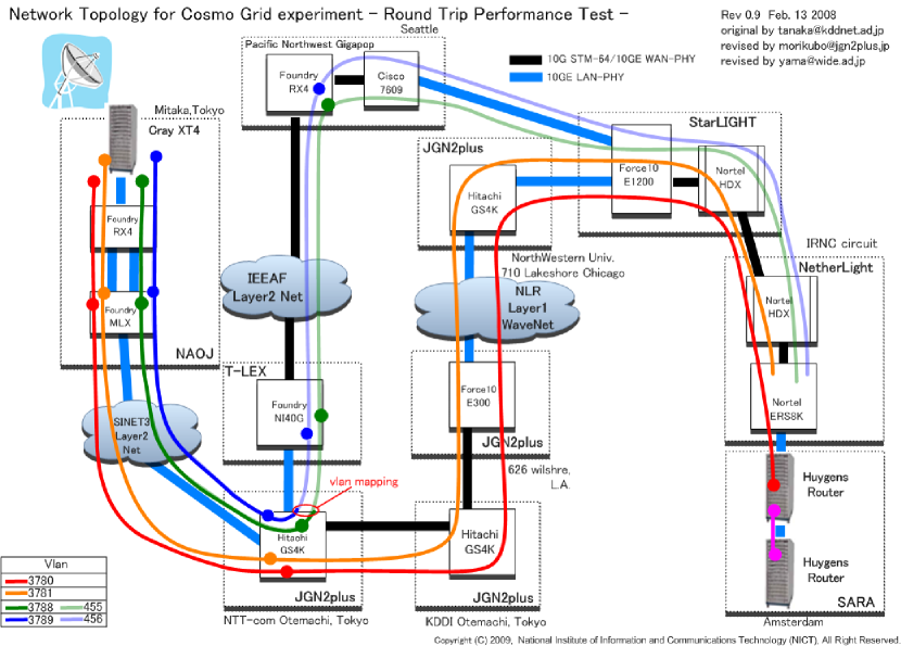
Figure 1: Network topology for the ComoGrid experimental setup. We used two main network connections between JGN2plus and StarLIGHT; one of then goes via L-LEX and Gigapop, the other connects directly from StarLIGHT to JGN2plus. Both paths have a network bandwidth of 10Gb/s, carried over 10 GE-LANPHY and 10 GE-WANPHY segments depending on the type of interfaces present at the various switching points. Thick blue lines (LANPHY) and thick black lines (WANPHY).

The network communication was realized by configuring two virtual LANs (vLAN) to create two paths connecting both supercomputers. One vLAN was used for the production traffic and runtime synchronization, while the second was configured for testing purposes and for collecting the simulation data at the PByte storage array in Amsterdam. Both paths are dedicated to our experiments which prevents packet loss, packet reordering and latency changes due to congestion. In the secondary path we had to execute vLANs translation in the JNG network, because the chosen vLANs numbers were unavailable along the entire path length. The choice of an available vLAN number for the end-to-end communication should have been trivial; but since our multi-domain light path lagged automatic configuration tools, human intervention was necessary. The time required for solving problems depends on the quick responses to email and phone calls, which is hindered by working over several time zones; debugging link failure at Layer2 in a multi-domain multi-vendor infrastructure is impractical and extremely time consuming. A self-healing or automatic setup would enormously help future experiments.

The Research and Education Networks (REN) provided the links for free, which is motivated by their vision to advertise and broaden their services to the scientific community. In the last few years many RENs have adopted a hybrid model for their architecture, expanding it to routed IP services where users have access to dedicated light paths in which communication occurs at lower layers of the open system-interconnection reference model. We settled for a flat Ethernet path, but still had to make the network reservations 3 weeks in advance of each simulation restart, and then it would generally take about a week before it was fully operational. Our overall experience with the use of light paths however, is quite positive. We could not have performed our calculation without this type of network setup and certainly perceived the advantage of the unrestricted and exclusive use of the links.

2.1 Demand on the network

While performing a cosmological $N$-body simulation in which the computational domain is shared by two (or more) computers, the positions and velocities of all particles on both machines have to be synchronized throughout the simulation. This introduces an enormous demand on the network between the computers. Luckily only a small boundary layer between the two halves of the universe and the layer nearest the periodic boundary are communicated between Amsterdam and Tokyo. The amount of data that has to be communicated per step is then

$$S_{\rm comm}=144N^{2/3}+4N_{p}^{3}+4N/S_{r}\,\,\,{\rm Byte}.$$ (1)

Here $N$ is the number of particles, $N_{p}$ is the resolution of the mesh in one dimension and $S_{r}$ is the sampling rate, which for the production simulation $S_{r}=5000$. The first term is required for communicating the tree structure, the second term is for exchanging the particles in the border region, and the last term is for exchanging the mesh. The first term in this estimate depends slightly on redshift ($z$) and on the opening angle in the treecode ($\theta$), but is accurate for $\theta=0.5$.

While running, dense dark-matter clumps may not be distributed evenly across the computational domain and load balancing is done by guaranteeing that the calculation time per step is the same on each computer, generating a variable boundary layer between the two computers. Where initially both computer resolve exactly half the universe, in due time one of the two computers tends to deal with a larger volume.

The communication within each of the supercomputers is realized by domain decomposition, using the Message Passing Interface (mpich [2]). To warrant efficient and stable data transfer we developed the parallel socket library MPWide to facilitate the communication outside the local MPI domains (Groen etal 2009, in preparation). This communication consists of data transfers between the local compute nodes and the local communication node, and for the data transfer over the light-path between the supercomputers.

The socket library is included in all processes, providing an interface similar to regular MPI. A static communication topology is established at startup which uses multiple tcp connection for each intra-cluster communication path and multiple tcp connections for paths between supercomputers. The concurrent use of multiple streams is realized by running a separate thread for each stream. For the smaller runs we used 16 tcp streams, and 64 streams for the larger runs (see Tab. 1).

3 The Simulation environment

We adopted the treePM code GreeM which was initially developed by [12] and rewritten by Ishiyama etal (in press) to run efficiently on the selected hardware. The equations of motion are integrated in co-moving coordinates using the leap-frog scheme with a shared but variable time-step. Good performance at sufficient accuracy is then achieved when the time step is at least an order of magnitude smaller than the crossing time in the densest halo [4]. Spurious relaxation effects in the high-density clumps are prevented by introducing a Plummer softening to the force, which is comparable to the local inter-particle distance.

Since most simulation time is spent in calculating the gravitational forces between particles, we optimize this operation using the single precision X86-64 Streaming SIMD Extensions (SSE). The inverse square-root SSE instruction provides the best speedup in calculating Newtonian gravity. We further improve performance by minimizing RAM access through the 16 XMM registers for the force operations, and by operating on pairs of two 64-bit floating point words concurrently (Nitadori & Yoshikawa in preparation).

With these optimizations the Power6 with symmetric multiprocessing is per core is about 4.2% slower than the Intel based Cray XT4. This small difference in speed is achieved by adopting the x86 SSE version and the Power AltiVec architectures, but for the former we use in-line assembly whereas for the latter we adopted the intrinsic functions (Nitadori & Yoshikawa in preparation).

We measure the performance of the code using the Amsterdam and Tokyo machines separately with $p=1$ to $p=1024$ processors and $N=256^{3}$ to $N=1024^{3}$ particles. The wall clock time $t_{\rm cpu}$ is then fitted by $t_{\rm cpu}\simeq 14,500p^{-0.91}$ seconds, with a ten fold increase of $t_{\rm cpu}$ for every increase of the number of particles by $2^{3}$. For relatively small $N$ we lose scalability with respect to the number of processors for $p\simeq 10^{3}$ and $N\ {\raise-2.15277pt\hbox{$\buildrel<\over{\sim}$}}\ 256^{3}$.

4 Simulating the Universe

We are interested in structures of kpc to Mpc size. To minimize the effect of the periodic boundary conditions on such dark matter distributions we selected our simulation box at $z=0$ to have sides of 30 Mpc. The initial dark-matter distribution is generated at $z\simeq 65$, assuming that the relation between the velocity and the potential in Zel’dovich approximation is the same as in the linear theory [6]. The density field is then realized by multi-scale Gaussian random fields, which is described in terms of its power spectrum and was generated using MPGRAFIC [9].

We further adopted cosmological parameters which are consistent the 5-year WMAP results [7]. For clarity we opted for the nearest round values, which yields: matter (including dark) density $\Omega_{m}=0.3$, dark energy density $\Omega_{\Lambda}=0.7$, the slope for the scalar perturbation spectrum $n_{s}=1.0$, and the amplitude of fluctuations $\sigma_{8}=0.8$. With these parameters the universe is about 13.7 billion years old and the Hubble constant $H_{0}\simeq 70$ km/s/Mpc.

We ran several realizations at different resolution (in mass as well as spatially) to measure the performance before we completed a simulation to $z=0$. An overview of the performed simulations is presented in Tab. 1.

N	$N_{p}$	p (A+T)	$t_{\rm tot}$	$t_{\rm cpu}$	$\eta_{p}$
16777216	128	30+30	31.2	23.58	1.51
134217728	256	30+30	116.8	105.7	1.81
134217728	256	60+60	71.9	58.8	1.64
134217728	256	120+120	53.0	36.8	1.39
1073741824	256	500+250	60.0	40.0	—
8589934592	256	500+250	380.0	310.0	—

Table 1: The performed simulations in a computational box of 30 Mpc starting at $z\simeq 65$, a softening of 300 pc and the opening angle in the tree-code $\theta=0.3$ for $z>10$ after which $\theta=0.5$. The first column gives the number of particles in the simulation followed by the number of mesh-cells in one dimension. Then we give the number of processors in Amsterdam (A) and Tokyo (T). The next two columns give the average wall-clock time for one step ($t_{\rm tot}$) and the time spent computing the forces ($t_{\rm cpu}$), both in seconds. The last two columns gives the speed-up $\eta_{p}$ which is defined as the wall-clock time of a single computer as fraction of the wall-clock time of the grid of supercomputers. Here we define $\eta_{p}$ for a grid where each computer has the same number of processors $p$. For the last two entries $\eta_{p}$ is then not properly defined.

The simulation with $N=16777216$ took about 10 hours to complete from $z\simeq 65$ to $z=0$. In Fig. 2 we show the wall-clock time of this run decomposed in the time spend in calculation, communication and storing the data to the file system. About 25% of the time is spent in communication (see Tab. 1), which is roughly constant through the simulation. We encountered a few problems between $z\simeq 16$ and $z\simeq 15$, which are probably related to packet loss in the network transport protocol suite and resulted in an additional performance loss of a few per-cent.

Figure 2: Wall-clock time as a function of redshift ($z$) for the simulation with $N=16777216$. The solid curve gives the wall-clock time, including the network wait stages, the dashed curve gives calculation time and the dotted curve indicates the time spend communicating. The lower thin dotted curve gives the time for storing data.

During the communication the speed of data transfer averages 21.1Mbit/s with peaks of about 7Gbit/s and per step between 16MB and 26MB is transferred. For the larger runs the average throughput increases to about 208Mbit/s since the size of the packages increases with $N$ (see Eq. 1).

The result of the simulation with $N=16777216$ at $z=0$ is presented in two panels in Fig. 3. Each of the two panels show the universe as it is seen by the two supercomputers, with the black parts on the right of the left panel (left on the right image) indicate the part of the universe that resides on the other machine.

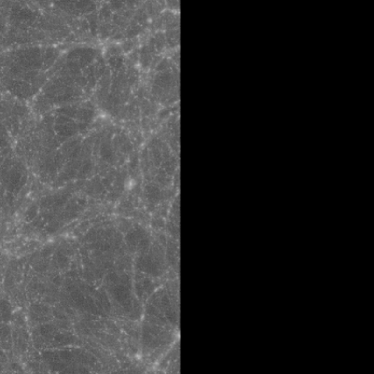
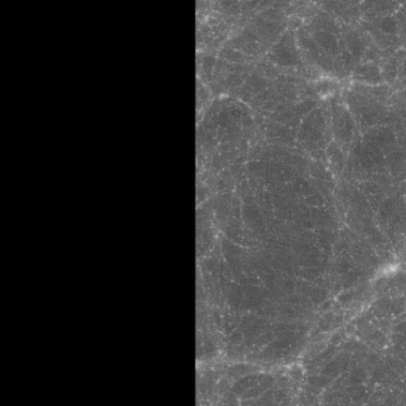
Figure 3: Final snapshot of the simulation with $N=256^{3}$ with Tokyo (left) and Amsterdam (right) . The black part of each figure represents the memory share that is located at the other site.

5 Concluding remarks

The formation of large scale structure in the universe can be studied effectively by means of simulation but requires phenomenal computer power. Even with fully optimized numerical methods and approximations the wall-clock time for such simulations can exceed several months. Our largest simulation with $N=8589934592$ has been running for about 1 million CPU hours (more than 1 month on 1024 processors) to reach $z\simeq 1.5$ and we expect to spend another $\sim 2$ million CPU hours to reach $z=0$.

The runs in Tab. 1 are performed on a grid of supercomputers. With our implementation the latency and throughput of the communication poses a relatively small overhead to the calculation cost, in our largest simulation the communication overhead $\ {\raise-2.15277pt\hbox{$\buildrel<\over{\sim}$}}\ 10$%. We have therewith demonstrated that large-scale structure formation simulations are excellently suited for high-performance grid computing.

The adopted setup would in principle have reduced our wall-clock time by almost a factor two compared to running on a single supercomputer, and our simulations in Tab. 1 have indeed effectively benefitted from using the grid. However, we have spend more than a year preparing and optimizing the code, and acquiring and scheduling the resources, none of which proved to be trivial. On the other hand, if we would not have opted for running on a grid it would have proven extremely difficult to perform the simulations at all since acquiring 1024 processors on a supercomputer for half-year via a ’normal’ proposal would be challenging. Even acquiring half the resources on two supercomputers with the promise to switch computers half-way the simulation would be difficult. Our strategy to run on a grid enabled us to secure the required CPU time on both supercomputers.

During this project we all became very enthusiastic about the computational grid as a high-performance resource, despite the time we have spend with preparations. The success of our grid is in part a consequence of the realization that latency forms no bottleneck, even if the computers are separated by half the planet. We cannot beat the speed of light, but bandwidth is likely to improve with time, making high-performance grid computing very attractive in the foreseeable future. Much work, however, is needed in improving practical matters, like scheduling issues, network acquisition and cooperation between supercomputer centers, each of which are major bottlenecks. We seriously consider to perform our next run on a grid with many supercomputers.

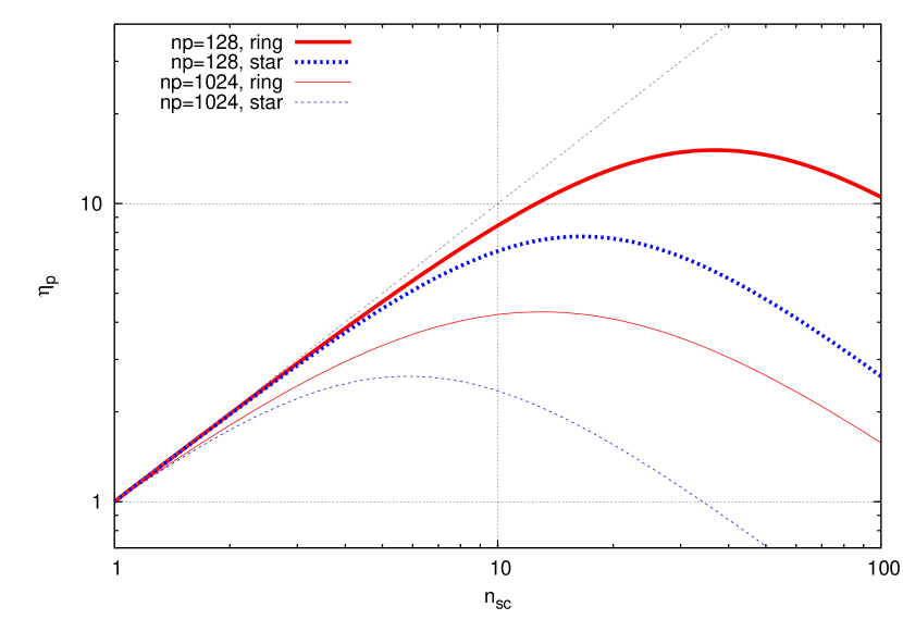
Figure 4: The speedup ($\eta_{p}$) for a grid of $n_{sc}$ supercomputers each with $p$ processors. The speedup is defined as the wall-clock time of the grid computer as fraction of the wall-clock time of one single supercomputer, assuming that each computer has $p$ processors. The thick curves are calculated with $p=128$ the thin curves with $p=1024$. The solid curves are calculated assuming the ring topology network, whereas for the dotted curves we adopted a star connected network. We adopted an average bandwidth of $b=200$ Mbyte/s with a latency of $\nu t_{\rm lat}=0.828$ s for the external (grid) communication and 10Gbyte/s for internal communication. The diagonal thin dashed curve indicates the ideal scaling.

Based on our measurements for each of the two supercomputers and the intercontinental grid we constructed a performance model, which is composed of two main components: the calculation ($t_{\rm cpu}$) and the data transfer over the grid $t_{\rm comm}=\nu t_{\rm lat}+S_{\rm comm}/b$, where $t_{\rm lat}$ is the network latency and $b$ is the network throughput (see Eq. 1). The parameter $\nu$ is introduced to correct for the inefficiencies in our code which require several transmissions ($\nu$) to the other computer. In Fig. 4 we present the results of the performance model based on the characteristics of the adopted computers, network and software environment for $N=2048^{3}$. The speedup is limited by the bandwidth, whereas latency, for which we adopted $t_{\rm lat}=0.138$s with $\nu=6$, poses no limiting factor to our simulations. Reducing the total latency will hardly improve the performance, but improving the throughput by a factor 10 would allow us to use an order of magnitude more processors per supercomputer while still acquiring acceptable speedup. The two topologies adopted in Fig. 4 are selected based on an ideal setup where the supercomputers are interconnected via a ring topology. A sub-optimal star topology leads to congestion as the communication tends to go through a single site. With the optimal topology (solid curves in Fig. 4) running on a 10 supercomputers with $\ {\raise-2.15277pt\hbox{$\buildrel<\over{\sim}$}}\ 128$ processors each results in a speed-up of a factor of $\sim 8$, whereas running on 100 supercomputers the speedup would be only a factor of 10.

The best strategy for performing cold dark matter simulations using a treePM code on a grid appears to be by acquiring $p\ {\raise-2.15277pt\hbox{$\buildrel<\over{\sim}$}}\ 100$ processors on $n_{\rm sc}\sim 10$ supercomputers in a ring network topology. The main reason for adopting this strategy would be to be able to acquire the required compute resources; it is considerably easier to obtain $p\sim 100$ processors for an extended period ($\sim 1$ year) from a dozen supercomputer centers, than to acquire the required CPU hours on a single supercomputer. This strategy, however, would require drastic changes in the co-scheduling policy of the supercomputer centers.

With our cosmological cold dark matter simulation we make the dream of Foster and Kesselman [1] comes true, our calculation benefits from having multiple widely separated computers interconnected with a high-bandwidth network, effectively operating as a single machine.

The authors

Simon Portegies Zwart

is professor in computational astrophysics at the Sterrewacht Leiden in the Netherlands. He received his Ph.D. in astronomy at Utrecht University. His principal scientific interests are high-performance computational astrophysics and the ecology of dense stallar systems.
e-mail:spz@strw.leidenuniv.nl,
URL:http://www.strw.leidenuniv.nl/$\sim$spz/

Tomoaki Ishiyama and Derek Groen

Are graduate students in the research groeps of Makino and Portegies Zwart, respectivly.

Jun Makino

is professor of astrophysics at the National Astronomical Observatory of Japan. He recieved his PhD in astronomy at the University in Tokyo. His research interests are stellar dynamics, large-scale scientific simulation and high-performance computing.
e-mail:makino@cfca.jp,
URL:http://www.artcompsci.org/$\sim$makino

Cees de Laat

is associate professor of system and network engineering at the University of Amsterdam. He recieved his PhD in computer science at the University of Amsterdam. His research interests are optical/switched Internet for data-transport in TeraScale eScience applications. e-mail:delaat@uva.nl,
URL:http://www.science.uva.nl/$\sim$delaat

Steve McMillan

is professor of physics at Drexel University in Philadelphia, Pennsylvania, U.S.A. He received his Ph.D. in astronomy from Harvard University. His principal scientific interests are high-performance computation and the astrophysics of star clusters and galactic nuclei.
e-mail:steve@physics.drexel.edu,
URL:http://www.physics.drexel.edu/$\sim$steve

Kei Hiraki

is professor in computer science at the University of Tokyo. He received his Ph.D. in phisics at the University of Tokyo. His research interests are parallel and distributed system, high-performance computing and networking.
e-mail:hiraki@is.s.u-tokyo.ac.nl,
URL:http://www-hiraki.is.s.u-tokyo.ac.jp

Stefan Harfst

is a postdoctoral fellow in the computational astrophysics group of Portegies Zwart. He received his Ph.D. in astrophysics at the University of Kiel, Germany. His research interests are stellar dynamics and high-performance computing.
e-mail:harfst@strw.leidenuniv.nl

Keigo Nitadori

Is a postdoctoral fellow at RIKEN, Japan. He received his Ph.D. in astrophysics at the University of Tokyo.
e-mail:keigo@riken.jp

Paola Grosso

is a senior researcher at the system and network engineering group at the University of Amsterdam. She received her Ph.D. in Physics from the University of Turin in Italy. Her research interests are modeling, programming and virtualization of networks for eScience applications.
e-mail:p.grosso@uva.nl,
URL:http://www.science.uva.nl/$\sim$grosso

References

- [1] Foster, I., C. Kesselman, and S. Tuecke, “The Anatomy of the Grid: Enabling Scalable Virtual Organizations,” ”International Journal of High Performance Computing Applications” 2001, 15, 200.
- [2] Gropp, W., E. Lusk, N. Doss, and A. Skjellum, “A high-performance, portable implementation of the MPI message passing interface standard,” Parallel Computing 1996, 22, 6, 789–828.
- [3] Guth, A. H., “Inflationary universe: A possible solution to the horizon and flatness problems,” Phys. Rev. D 1981, 23, 347–356.
- [4] Hockney, R. and J. Eastwood, Computer Simulation Using Particles, Adan Hilger Ltd., Bristol, UK, 1988, 540 pp.
- [5] Hoekstra, G., A., S. Portegies Zwart, M. Bubak, and P. Sloot, Towards Distributed Petascale Computing, Petascale Computing: Algorithms and Applications, by David A. Bader (Ed.). Chapman & Hall/CRC computational science series 2008, 565pp.
- [6] Joyce, M. and B. Marcos (2007), “Quantification of discreteness effects in cosmological N-body simulations. II. Evolution up to shell crossing,” Phys. Rev. D 76, 10, 103505.
- [7] Komatsu, E., J. Dunkley, M. R. Nolta, C. L., “Five-Year Wilkinson Microwave Anisotropy Probe (WMAP) Observations: Cosmological Interpretation,” 2008, ArXiv e-prints 803.
- [8] Lee, B. W. and S. Weinberg (1977), “Cosmological lower bound on heavy-neutrino masses,” Physical Review Letters 39, 165–168.
- [9] Prunet, S., C. Pichon, D. Aubert, D. Pogosyan, R. Teyssier, and S. Gottloeber, “Initial Conditions For Large Cosmological Simulations,” ApJS 2008, 178, 179–188.
- [10] Spergel, D. N., R. Bean, O. Doré, et la. “Three-Year Wilkinson Microwave Anisotropy Probe (WMAP) Observations: Implications for Cosmology,” ApJS 2007, 170, 377–408.
- [11] Xu, G., “A New Parallel N-Body Gravity Solver: TPM,” ApJS 1995, 98, 355.
- [12] Yoshikawa, K. and T. Fukushige, “PPPM and TreePM Methods on GRAPE Systems for Cosmological N-Body Simulations,” Publ. Astr. Soc. Japan 2005, 57, 849–860.