A Deep Chandra X-ray Spectrum of the Accreting Young Star TW Hydrae

Abstract

We present X-ray spectral analysis of the accreting young star TW Hydrae from a 489 ks observation using the Chandra High Energy Transmission Grating. The spectrum provides a rich set of diagnostics for electron temperature $T_{e}$, electron density $N_{e}$, hydrogen column density $N_{H}$, relative elemental abundances and velocities and reveals its source in 3 distinct regions of the stellar atmosphere: the stellar corona, the accretion shock, and a very large extended volume of warm postshock plasma. The presence of Mg XII, Si XIII, and Si XIV emission lines in the spectrum requires coronal structures at $\sim$10 MK. Lower temperature lines (e.g., from O VIII, Ne IX, and Mg XI) formed at 2.5 MK appear more consistent with emission from an accretion shock. He-like Ne IX line ratio diagnostics indicate that $T_{e}=2.50\pm 0.25$MK and $N_{e}=3.0\pm 0.2\times 10^{12}$ cm^-3 in the shock. These values agree well with standard magnetic accretion models. However, the Chandra observations significantly diverge from current model predictions for the postshock plasma. This gas is expected to cool radiatively, producing O VII as it flows into an increasingly dense stellar atmosphere. Surprisingly, O VII indicates $N_{e}=5.7^{+4.4}_{-1.2}\times 10^{11}$ cm^-3, five times lower than $N_{e}$ in the accretion shock itself, and $\sim$ seven times lower than the model prediction. We estimate that the postshock region producing O VII has roughly 300 times larger volume, and 30 times more emitting mass than the shock itself. Apparently, the shocked plasma heats the surrounding stellar atmosphere to soft X-ray emitting temperatures and supplies this material to nearby large magnetic structures – which may be closed magnetic loops or open magnetic field leading to mass outflow. Our model explains the soft X-ray excess found in many accreting systems as well as the failure to observe high $N_{e}$ signatures in some stars. Such accretion-fed coronae may be ubiquitous in the atmospheres of accreting young stars.

1. Introduction

Low mass stars in star-forming regions produce strong X-ray emission from coronal magnetic activity, as evidenced by high temperature ($\sim$10 MK) emission from flares and active regions (Feigelson & Montmerle 1999; Gagné et al.  2004; Preibisch et al.  2005). The role of accretion in the production of X-rays from young stars is less well understood. Magnetic structures on stars can extend all the way to the inner accretion disk, as suggested from models of decaying stellar flares (Favata et al.  2005). Extended X-ray emission from jets also occurs, as observed in DG Tau, a system oriented so that the circumstellar disk plane aligns with our line of sight (Güdel et al. 2008). Soft X-ray emission may arise from shocks at the stellar base of this extended X-ray jet (Güdel et al.  2008; Schneider & Schmitt 2008).

X-rays can also be produced in accreting systems when the accreting material accelerates to supersonic velocities and shocks near the stellar surface, heating the gas to a few MK. In the standard model of accreting Classical T Tauri Stars (CTTS), the magnetic field of the star connects to the accretion disk near the corotation radius, channeling the accretion stream from the disk to a small area on the star (Calvet & Gullbring 1998). X-rays from the shock may be difficult to detect if the shock is formed too deep in the photosphere (Hartmann 1998) or if they are absorbed by the stream of preshocked neutral or near-neutral gas. Furthermore, the X-ray shock signature may be difficult to distinguish from soft coronal emission without the high resolution spectroscopy necessary to determine temperature and density and identify the emitting regions. Shock models predict high electron density $N_{e}$ ($\sim 10^{13}$ cm^-3) at relatively low electron temperature $T_{e}$ (a few MK), features that can be tested with X-ray line ratio diagnostics.

TW Hydrae (TW Hya) was the first CTTS found to show these characteristics of high density and low temperature (Kastner et al. 2002; hereafter, K02), based on a 48 ks Chandra High Energy Transmission Grating (HETG) spectrum. TW Hya is one of the oldest known stars ($\sim$ 10 Myr) still in the CTTS (accreting) phase. It is uniquely poised in an interesting state of evolution when it will soon stop accreting, lose its disk, and perhaps form planets (e.g., Calvet et al.  2002). At a distance of only 57 pc, it is also one of the brightest T Tauri stars in X-rays. Interstellar absorption is minimal, and the observed absorption can be considered intrinsic to the system (K02). TW Hya’s circumstellar disk is nearly face-on with an inclination angle of 7^o (Qi et al. 2004). Thus the star appears pole-on.

Key to K02’s argument for accretion is the electron density ($N_{e}\sim 6\times 10^{12}$ cm^-3) determined from He-like Ne IX emission line ratios, and confirmed by subsequent observations with the XMM-Newton Reflection Grating Spectrometer (Stelzer & Schmitt 2004) and the Chandra Low Energy Transmission Grating (LETG; Raassen 2009). While $N_{e}$ for some active cool star coronae approaches such high values at high $T_{e}$ ($\sim 10$ MK), e.g., 44 Boo, UX Ari, and II Peg (Sanz-Forcada et al.  2003; Testa et al.  2004), the high $N_{e}$ of TW Hya is produced at the significantly lower $T_{e}$ ($\sim$3 MK) expected for the accretion shock. BP Tau (Schmitt et al.  2005), V4046 Sag (Gunther et al.  2006), RU Lup (Robrade & Schmitt 2007), and MP Mus (Argiroffi et al.  2007) also show high values of the electron density. On the other hand, T Tau and AB Aur have a low $N_{e}$ (Güdel et al.  2007a; Robrade & Schmitt 2007); and, the binary Hen 3-600 appears to lie at an intermediate value of $N_{e}$ (Huenemoerder et al.  2007). Despite large differences in $N_{e}$, all of these stars show an excess ratio of soft X-ray emission to hard X-ray emission, manifested by their large O VII/O VIII ratios as compared with active main sequence stars (Güdel & Telleschi 2007; Robrade & Schmitt 2007). Additional soft X-ray diagnostics available with a deep Chandra exposure might be expected to shed light on the accretion process and test the shock models.

Since accretion is expected to result in higher densities than found in an active stellar corona, it is critical that the density determination be secure. Interpretation of the Ne IX line ratio in terms of high density is not unique, since photoexcitation by ultraviolet radiation mimics the effects of high density. Determining the density from Mg XI is not subject to the same degeneracy, since the relevant ultraviolet radiation, observed with the Far Ultraviolet Explorer (FUSE; Dupree et al.  2005), is too weak to photoexcite its metastable level. The three He-like systems (O VII, Ne IX, and Mg XI) together can provide independent determinations not only of the electron density, but also of the electron temperature and hydrogen column density. Deep spectroscopy can, first, put the accretion interpretation on firm ground and second, allow us to determine the structure of the accretion region itself.

We were awarded a Chandra Large Observing Project to establish definitively whether the X-ray emission in TW Hya is associated with accretion, using high signal-to-noise ratio spectroscopy with the HETG, and, if so, to determine the emission measure distribution and elemental abundances, search for X-ray signatures of infall, outflow, and turbulence, and constrain the properties of the accretion hot spot. During the Chandra observations we also conducted a ground-based observing campaign, which will be reported elsewhere (Dupree et al.  2010, in preparation). Here, we describe the X-ray observations in Section 2 and report analysis results in Section 3, where the densities, temperatures, and column densities can be extracted from this rich spectrum. Section 3 also presents elemental abundances derived from fits to the spectrum, as well as the measurement of turbulent velocity. Section 4 describes spectral predictions from a model of the TW Hya shock. In Section 5 we discuss evidence for a new type of coronal structure. Section 6 gives a summary of results and conclusions.

2. Observations and Spectral Analysis

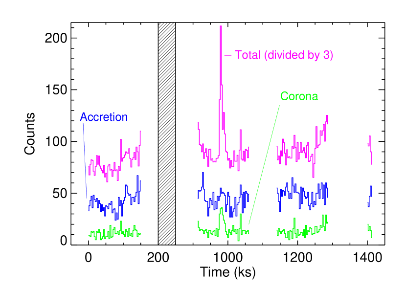
Chandra observed TW Hya with the HETG in combination with the ACIS-S detector array for a total of 489.5 ks intermittently spanning the period between 2007 Feb 15 and 2007 Mar 3. The observation consists of 4 segments, with exposure times as follows: 153.3 ks (Obsid 7435), 157.0 ks (Obsid 7437), 158.4 ks (Obsid 7436), and 20.7 ks (Obsid 7438). The summed spectrum has about ten times the exposure time of the spectrum analyzed by K02. Figure 1 shows the total first-order light curve, with flux variations of about a factor two during the observation. Assuming a distance of 57 pc, the observed X-ray luminosity $L_{X}$, measured using the Medium Energy Grating between 2.0 and 27.5 Å, is $1.3\times 10^{30}$ erg s^-1. One clear flare, with total X-ray luminosity of 2.1 $\times 10^{30}$ erg s^-1, persists for $\sim$15 ks, producing a total energy of 4 $\times 10^{34}$ ergs. The flare is retained in the following analysis since its contribution to line fluxes is negligible (see Section 3.4).

Figure 1.— X-ray light curves (first order counts vs time since start) for the four observing segments of the Chandra observation. The hashed area represents a gap of 650 ks. The upper curve shows the light curve for the total first order counts. This light curve includes both line and continuum emission. The middle curve uses the combined line counts from N VII, O VII, O VIII, Ne IX, Fe XVII, and Mg XI (identified as the “accretion” lines using Model D, discussed in Section 3.4). The lower curve uses the combined line counts from Mg XII, Si XIII, and Si XIV (identified as the lines from the “corona” from Model D). Note that the line-based light curves also include any continuum counts within the line profile. The data are binned over 3 ks.

We have extracted spectra from the event files, and produced calibration files using the Chandra Interactive Analysis of Observations (CIAO ver. 3.4) software package (Fruscione et al.  2006). With response matrices combined from the four observations, Sherpa (Freeman et al.  2001) was used to extract individual emission line fluxes from the co-added observations, maintaining separate first order spectra for the four grating arms (plus and minus; MEG and HEG) during the fitting procedure. A model for the continuum plus background was found from a global fit to line-free regions and used in addition to the line models. Background rejection is high with ACIS order sorting. Thus the background contributes relatively little to this model except at the long wavelength end of the spectrum, where the effective area is low. In the O VII region, for example, the background contains about half as many counts as the continuum. For the relatively weak but important O VII line, background, continuum, and line have about 1, 2, and 16 counts, respectively.

Line models are Gaussian functions with negligible or small widths relative to the width of the instrumental line response functions ($\sim$0.012 Å and 0.023 Å, for HEG and MEG, respectively). Table 1 gives the identified lines and their observed fluxes. For most lines the fit widths are less than half the instrumental width and are not statistically significant. We discuss the widths of the strongest lines in Section 3.5.

Table 1Selected Emission Lines

Line	$\lambda_{ref}$	Flux	Eff Area	Origin
	(Å)	(10-6 ph cm-2 s-1)	(cm2)
Si XIV	6.182	1.87 $\pm$ 0.19	163.0	corona
Si XIII	6.648	2.72 $\pm$ 0.17	146.6	corona
Si XIII	6.688	0.74 $\pm$ 0.14	138.3	corona
Si XIII	6.740	1.66 $\pm$ 0.15	151.6	corona
Mg XII	8.421	2.24 $\pm$ 0.20	162.4	corona
Mg XI	9.169	2.25 $\pm$ 0.22	135.4	shock
Mg XI	9.231	0.90 $\pm$ 0.17	133.2	shock
Mg XI	9.314	1.27 $\pm$ 0.19	130.1	shock
Ne X	9.481	1.64 $\pm$ 0.20	114.5	corona
Ne X	9.708	2.75 $\pm$ 0.27	86.2	corona
Ne X	10.239	9.23 $\pm$ 0.53	81.1	corona
Ne IX	10.765	3.54 $\pm$ 0.43	67.9	shock
Ne IX	11.001	8.48 $\pm$ 0.63	67.4	shock
Ne IX	11.544	23.7 $\pm$ 0.99	55.3	shock
Fe XXII	11.783	3.28 $\pm$ 0.50	52.3	corona
Fe XXII	11.932	3.01 $\pm$ 0.50	49.6	corona
Ne X	12.134	76.1 $\pm$ 1.9	48.5	corona
Fe XVII	12.266	4.3 $\pm$ 0.6	46.6	mixed
Ne IX	13.447	177. $\pm$ 4.2	22.3	shock
Ne IX	13.553	114. $\pm$ 3.3	22.7	shock
Ne IX	13.699	58.7 $\pm$ 2.3	25.0	shock
Fe XVIII	14.208	4.59 $\pm$ 0.76	29.0	corona
Fe XVIII	14.256	1.63 $\pm$ 0.53	28.5	corona
O  VIII	14.820	5.04 $\pm$ 0.80	23.7	shock
Fe XVII	15.014	36.5 $\pm$ 1.8	21.9	shock
O  VIII	15.176	10.4 $\pm$ 1.2	20.8	shock
Fe XVII	15.261	17.4 $\pm$ 1.4	20.0	shock
O  VIII	16.006	30.6 $\pm$ 2.3	15.9	shock
Fe XVIII	16.071	5.17 $\pm$ 1.0	16.3	corona
Fe XVII	16.780	25.5 $\pm$ 3.0	12.1	shock
Fe XVII	17.051	27.9 $\pm$ 2.3	11.1	shock
Fe XVII	17.096	26.3 $\pm$ 2.3	11.2	shock
O  VII	17.207	4.68 $\pm$ 1.4	10.7	shock
O  VII	17.396	4.68 $\pm$ 1.5	9.8	shock
O  VII	17.768	3.66 $\pm$ 1.6	7.7	shock
O  VII	18.627	17.9 $\pm$ 1.4	7.3	shock
O  VIII	18.969	213. $\pm$ 8.4	6.6	shock
N  VII	20.910	3.8 $\pm$ 2.5	3.3	shock
O  VII	21.601	117. $\pm$ 10.0	2.8	postshock
O  VII	21.804	72.4 $\pm$ 9.1	2.7	postshock
O  VII	22.098	15.2 $\pm$ 4.4	2.1	postshock
N  VII	24.781	68.5 $\pm$ 7.6	2.6	shock

All line fluxes are within 3$\sigma$ of the values reported by K02 except for Ne IX $\lambda$13.437, which has slightly more than twice as much flux in our observation. Our line fluxes are also within 3$\sigma$ of the values reported by Stelzer & Schmitt (2004) for lines observed with both instruments, except for Ne IX $\lambda$13.553, for which our flux is about half. For lines in common with those reported by Raassen (2009) all fluxes agree within 3$\sigma$. With the higher signal-to-noise ratio of our data, new diagnostic information is available.

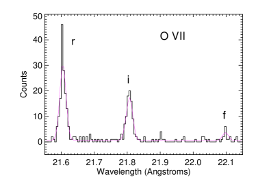
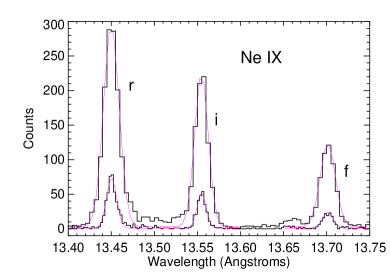
A major goal of this study is the determination of electron density from the He-like ions. We first discuss the diagnostics, and then model the global spectrum. Figure 2 shows the high quality in the He-like O VII and Ne IX line regions. Interestingly, the Ne IX region shows no apparent Fe XIX lines, which can contaminate the Ne IX diagnostics (e.g., Ness et al.  2003). Upper limits on the strongest Fe XIX line at 13.52 Å imply that Fe XIX contributes 1% or less to the Ne IX line fluxes.

Figure 2.— Top: Observed MEG spectrum in the O VII spectral region, shown as a histogram, with best-fit model (3 Gaussian lines) overlaid. Wavelength positions are fixed relative to each other and the instrumental line response function is included in the model. Resonance (r), intercombination (i) and forbidden (f) lines are marked. Bottom: Observed MEG (upper) and HEG (lower) spectra in the Ne IX region, shown as histograms, with best-fit model overlaid. For this fit, the positions, fluxes and line widths are free parameters, yielding the constraints on velocities described in the text.

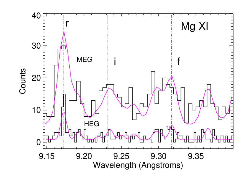
The Mg XI triplet line region is more complex (Fig. 3), with lower signal-to-noise ratio and apparent line blending between 9.2 and 9.4 Å. For this region, the fit is constrained such that all known lines are fixed in wavelength relative to the Mg XI resonance line $\lambda$9.169, which is fit separately for each grating arm. Lines are Gaussian functions with widths set to zero (i.e., only the instrumental line response function is used). Line fluxes of the Ne X Lyman series lines $n=5$ to $10$ are scaled according to their oscillator strengths, since collision strengths are not available in the literature. We note that systematic errors from line blends are not included in the errors given in Table 1.

3. Results

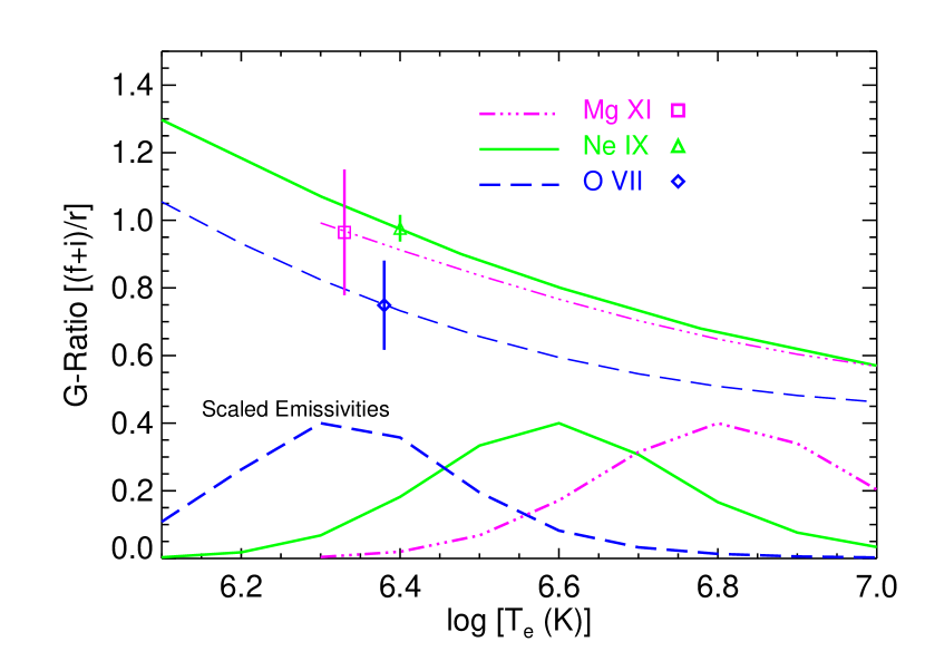
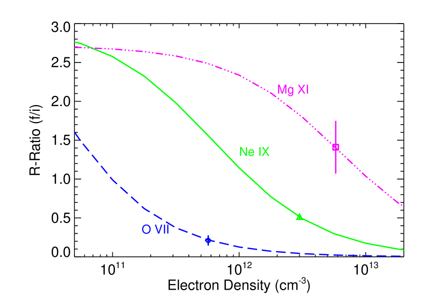
One of the advantages of X-ray spectroscopy with high signal-to-noise characteristics is the availability of numerous line ratio diagnostics to assess conditions in the radiating plasma. In particular, He-like systems provide valuable diagnostic opportunity, as discussed extensively in the literature (Porquet et al.  2001; Smith et al.  2001; and references therein). The G-ratio, defined as the flux ratio of the forbidden ($1s2s~{}^{3}S_{1}\rightarrow 1s^{2}~{}^{1}S_{0}$) plus intercombination ($1s2p~{}^{3}P_{1,2}\rightarrow 1s^{2}~{}^{1}S_{0}$) lines to the resonance ($1s2p~{}^{1}P{{}_{1}}\rightarrow 1s^{2}~{}^{1}S_{0}$) line, is sensitive to the electron temperature ($T_{e}$), while the R-ratio (flux ratio of the forbidden to intercombination lines) is sensitive to $N_{e}$. Ratios of emission lines in the resonance line series (transitions from 2p, 3p, etc. to ground, also known as He_α, He_β, and so on) are sensitive both to $T_{e}$, through their relative Boltzmann factors, and to the absorption by an intervening hydrogen column density ($N_{H}$) through their energy separation.

Figure 3.— Observed MEG (upper) and HEG (lower) spectra in the Mg XI spectral region, shown as histograms, with best-fit model spectrum, described in text, overlaid. Positions of resonance (r), intercombination (i), and forbidden (f) lines are marked.

This analysis emphasizes the use of line ratio diagnostics, including those discussed above. We use the Astrophysical Plasma Emission Code (APEC) with the atomic data in ATOMDB v1.3 (Smith et al.  2001) to calculate line emissivities, except for He-like Ne IX, for which we use the more accurate calculations of Chen et al.  (2006). The model for absorption by gas with cosmic abundances is taken from Morrison & McCammon (1983).

In this section we present the physical conditions of the emitting plasma as determined from the line ratios of specific He-like and other ions, in particular $N_{e}$, $T_{e}$, and $N_{H}$. We use information determined from line ratios to constrain an empirical model of the emission measure distribution (EMD), and then allow additional parameters of the model to be constrained by global fits to the spectrum. We give the elemental abundances determined from these fits. Finally we present velocity constraints from line centroids and widths.

3.1. Electron temperature

We use G-ratios from multiple ions to determine the electron temperature. Figure 4 shows the observed G-ratios of He-like O, Ne and Mg, overplotted on their respective theoretical functions of $T_{e}$. For comparison, the emissivities of their resonance lines peak at $T_{e}=$ 2, 4, and 6 MK, respectively, as shown in the figure. Table 2 gives the derived $T_{e}$ from these ions. The Ne IX G-ratio indicates that $T_{e}=2.5\pm 0.25$ MK. The Ne IX $T_{e}$ determination is highly reliable, given that recent theoretical calculations, which include the resonance contributions to the collisional excitation cross sections, agree with experimental measurements to within 7% (Chen et al.  2006; Smith et al.  2009a, 2009b). On the other hand, the theoretical calculations for O VII and Mg XI have higher systematic uncertainties, and the observational errors are larger, such that the $T_{e}$ values derived from O VII and Mg XI carry less weight (but are consistent with Ne IX). Both Ne IX and Mg XI are found far below their temperature of maximum emissivity $T_{max}$, supporting an accretion shock scenario for their formation.

Figure 4.— Theoretical G-ratios (i.e., ratios of forbidden plus intercombination to resonance line fluxes) as functions of $T_{e}$, for O VII (dashed), Ne IX (solid), and Mg XI (dash-dotted). Overplotted are the observed ratios with 1$\sigma$ errors. The model for Ne IX is from Chen et al.  (2006). The models for O VII and Mg XI are from APEC using ATOMDB v1.3 (Smith et al.  2001). Scaled emissivities (ph cm³ s^-1) for the resonance lines of the three ions are also shown. For Ne IX and Mg XI the derived temperatures are well below the temperatures of their peak emissivities, consistent with an intepretation of their formation in an accretion shock.

Table 2He-like G-Ratio $T_{e}$ Diagnostics

Ion	Observed Ratio	$T_{e}$
		(K)
O VII	0.75$\pm$0.13	2.4${}^{+1.2}_{-0.6}\times 10^{6}$
Ne IX	0.98$\pm$0.04	2.5${}^{+0.25}_{-0.25}\times 10^{6}$
Mg XI	0.97$\pm$0.19	2.1${}^{+2.1}_{-0.5}\times 10^{6}$

3.2. Electron density

We use R-ratios from multiple ions to determine the electron density. Figure 5 shows the observed R-ratios for O VII, Ne IX, and Mg XI, overplotted on the theoretical functions of electron density $N_{e}$ from APEC. Table 3 presents the $N_{e}$ values derived from these R-ratios. Sensitivity to $T_{e}$ is negligible near the observed R-ratio values. Smith et al.  (2009) show that the APEC R-ratio for Ne IX in the high density range is indistinguishable from the R-ratio calculated by Chen et al.  (2006). The theoretical R-ratios from APEC for all three ions are in excellent agreement with Porquet et al.  (2001) over the density range reported here.

Table 3He-like R-Ratio $N_{e}$ Diagnostics

Ion	Observed Ratio	$N_{e}$
		(cm-3)
O VII	0.21$\pm$0.07	5.7${}^{+4.4}_{-1.2}\times 10^{11}$
Ne IX	0.51$\pm$0.03	3.0${}^{+0.2}_{-0.2}\times 10^{12}$
Mg XI	1.41$\pm$0.34	5.8${}^{+3.8}_{-2.4}\times 10^{12}$

From Ne IX we derive $N_{e}=3.0\pm 0.2\times 10^{12}$ cm^-3, while O VII gives $N_{e}=5.7^{+4.4}_{-1.2}\times 10^{11}$ cm^-3. The 3$\sigma$ range from Ne IX, between 2.5 and 3.9 $\times 10^{12}$ cm^-3, provides a tight constraint. The best-fit value for Mg XI, using all the lines in the region as described in Section 2, is $N_{e}=5.8^{+3.8}_{-2.4}\times 10^{12}$ cm^-3. For comparison, we have also fit only the 3 lines of Mg XI, again with line widths and relative positions fixed, obtaining $N_{e}=$ 7 $\pm$ 2 $\times 10^{12}$ cm^-3, in good agreement with the best-fit value. This comparison suggests that line blending does not unduly affect the result.

Figure 5.— Theoretical R-ratios (i.e., ratios of forbidden to intercombination line fluxes) as functions of $N_{e}$ for He-like O, Ne and Mg. Overplotted are the observed ratios with 1$\sigma$ errors. Models are from APEC using ATOMDB v1.3. While Figure 4 shows that these ions are formed at similar temperature, they are found at significantly different densities.

At low $N_{e}$ the population of the metastable $2s~{}^{3}S_{1}$ level builds up since the decay rate is extremely low. At high $N_{e}$ electron impact excites the metastable level population up to the $2p^{3}P$ levels. In principle, low R-ratios may also be produced at low $N_{e}$ by photoexcitation. Stelzer & Schmitt (2004) and K02 dismiss photoexcitation based on the stellar temperature ($\sim$ 4000 K), but Drake (2005) suggests that a hot spot above the stellar surface, where the accretion stream shocks, could produce sufficient photoexciting radiation. We have measured the flux at the excitation wavelengths 1647 Å, 1270 Å and 1034 Å for O VII, Ne IX, and Mg XI, respectively, from the Hubble Space Telescope STIS (Herczeg et al.  2002) and the FUSE spectra (Dupree et al.  2005). The intensity at 1034 Å is an order of magnitude lower than at the longer wavelengths, constraining the black body temperature of the hot spot to be less than 10,000 K, in good agreement with International Ultraviolet Explorer analysis showing a blackbody at 7900 K covering about 5% of the stellar surface (Costa et al.  2000). Thus the ultraviolet measurements and the Mg XI R-ratio rule out photoexcitation and support the interpretation of high $N_{e}$. Together with the temperature derived from the Ne IX G-ratio, the density supports an accretion origin for Ne IX.

The ratio of Fe XVII $\lambda$17.096 to $\lambda$17.051 becomes sensitive to $N_{e}$ above $\sim 10^{13}$ cm^-3 (Mauche et al. 2001). The measured ratio of 1.06 $\pm$ 0.13 is at the low $N_{e}$ limit, ruling out the high density from this line ratio suggested by Ness & Schmitt (2005).

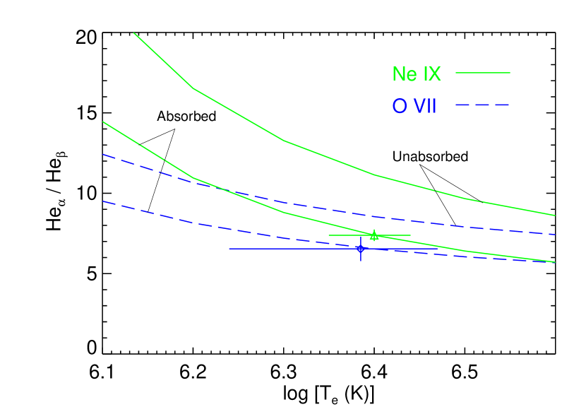
3.3. Hydrogen column density

The HETG spectrum contains several series of resonance lines that indicate absorption by neutral gas along the line of sight. The most useful of these diagnostics are the O VII and Ne IX He_α/He_β ratios because their formation temperatures are independently determined from the G-ratio. Table 4 presents the observed line ratios, and their use as diagnostics for $N_{H}$. Figure 6 shows the theoretical He_α/He_β ratios as functions of $T_{e}$ for O VII and Ne IX, for both unabsorbed and absorbed cases. The observed ratios are overplotted using $T_{e}$ determined from their G-ratios (which, as noted above, is more reliable for Ne IX than for O VII). For the best-fit $T_{e}$, Ne IX gives $N_{H}=1.8\pm 0.2\times 10^{21}$ cm^-2 and O VII gives $N_{H}=4.1^{+1.9}_{-1.6}\times 10^{20}$ cm^-2. These two values show a meaningful difference. For Ne IX at 2.5 MK, the observed ratio is 11$\sigma$ below the unabsorbed model, making the presence of an absorbing column quite definitive. The column density from O VII is consistent with the lower limit of $N_{H}=2\times 10^{20}$ cm^-2 determined from the absence of Ne VIII and Si XII lines longward of 40 Å in the Chandra LETG spectrum (Raassen 2009).

Table 4Line Ratio $N_{H}$ Diagnostics

Identification	Observed	Predicted Ratio for log $N_{H}$ (cm-2):
	Ratio	0.00	20.61	20.89	21.26
O VII He$\alpha$/He$\beta$	6.54$\pm$0.76	8.54	6.52	5.22	2.49
O VIII Ly$\alpha$/Ly$\beta$	6.95$\pm$0.58	9.63	8.07	6.82	4.55
Ne IX He$\alpha$/He$\beta$	7.38$\pm$0.35	11.14	10.07	9.23	7.34
Ne X Ly$\alpha$/Ly$\beta$	8.24$\pm$0.52	12.93	11.89	10.91	8.93
Ne X Ly$\alpha$/Ly$\beta$	8.24$\pm$0.52	7.061	6.49	5.96	4.88

Figure 6.— Theoretical models of He_α to He_β line flux ratios as functions of $T_{e}$, with solid curve for Ne IX and dashed curve for O VII. The filled circle is the observed ratio for Ne IX and the open circle is for O VII, with 1$\sigma$ error bars. Unabsorbed and best absorbed models for each ion are labeled. The absorbed models shown have $N_{H}=1.8\times 10^{21}$ and $4.1\times 10^{20}$ cm^-2 for Ne IX and O VII, respectively.

Ratios of the H-like series lines (Ly_α, Ly_β, etc.) are also sensitive to both absorption and temperature, but unlike the He-like ions, H-like ions do not present an independent temperature diagnostic. If the absorption column depends on the ion, as implied by the inconsistency between Ne IX and O VII, then we need to assume a model $T_{e}$ to obtain a column density from the H-like line ratios. Assuming 2.5 MK, the observed ratio O VIII Ly_α/Ly_β indicates $N_{H}=7.8^{+1.1}_{-0.9}\times 10^{20}$ cm^-2. This value is consistent within the errors with $N_{H}$ from O VII and thus a third absorber is not required. For Ne X at 2.5 MK, the column density would be larger than the column density for Ne IX, as shown in Table 4; however, Table 4 also shows that no absorption is required if the Ne X lines are formed at 10 MK. We must further consider the effects of temperature on Ne X line ratios.

We can also estimate the temperature using the charge state balance. Table 5 presents the He_α/Ly_α ratios for oxygen and neon. First, the observed ratios are corrected for different column densities as found above, and then $T_{e}$ is derived from the respective corrected ratios. For oxygen, good consistency is found for the temperatures derived from the G-ratio and the O VII He_α/O VIII Ly_α ratio, given a column density of about 8 $\times 10^{20}$ cm^-2. For neon, on the other hand, all the derived temperatures are larger than $T_{e}$ derived above from the Ne IX G-ratio. Thus it appears that some of the Ne X emission originates at higher temperature. Using $N_{H}=2\times 10^{21}$ cm^-2 and $T_{e}=2.5$ MK, and the observed Ne IX He_α flux, we predict the flux of the Ne X Ly_α to be only 18% of the observed value. In this case, the rest of the Ne X emission must be formed at higher temperature. If the trend of increasing $N_{H}$ with charge state continues, then $N_{H}$ for Ne X would be higher than $2\times 10^{21}$ cm^-2, and the fraction of Ne X formed at 2.5 MK would be somewhat larger.

Table 5$T_{e}$ From Charge State Balance

Identification	Observed	Corrected for log $N_{H}$ (cm-2):
		20.61	20.89	21.26
O VII He$\alpha$/O VIII Ly$\alpha$	0.55$\pm$0.052	0.70	0.85	1.67
Ne IX He$\alpha$/Ne X Ly$\alpha$	2.32$\pm$0.08	2.48	2.60	3.04
Identification	Derived $T_{e}$ ($10^{6}$ K)
O VII He$\alpha$/O VIII Ly$\alpha$	3.03	2.83	2.66	2.23
Ne IX He$\alpha$/Ne X Ly$\alpha$	4.16	4.08	4.01	3.87

The emissivity functions for lines of Fe XVII and Ne X both peak near 5 MK, suggesting the possibility of comparing their formation temperatures. The ratio of Fe XVII $\lambda$15.014 to $\lambda$15.261 is sensitive to $T_{e}$, due to a blend of an inner shell excitation line of Fe XVI at 15.261 Å (Brown et al.  2001). The temperature sensitivity essentially comes from the charge state balance of Fe XVI and Fe XVII. Using the reported experimental dependence of the line ratio on the electron beam energy of the Electron Beam Ion Trap at Lawrence Livermore National Laboratory (Brown et al.  2001), the observed HETG value gives $T_{e}=2.34^{+0.09}_{-0.06}$ MK. Despite similar peak temperatures, Fe XVII and Ne X are not formed together. Apparently, the long tail of the Ne X Ly_α emissivity function toward high temperature contributes significantly to its emission. The Fe XVII lines are predominantly formed in the accretion shock, while the Ne X lines are formed both in the shock and in the hotter corona.

One might expect that the ions formed at low temperature (O VII, O VIII, and Ne IX) should all experience similar absorption. Using $N_{H}$ derived from Ne IX, we can derive characteristic emitting $T_{e}$ for O VIII and O VII of 1.4 MK and $<1.0$ MK, respectively. These temperatures are far lower than $T_{e}$ derived from the O VII G-ratios. They are both also far lower than $T_{e}>2$ MK derived from the charge state ratio of oxygen represented over the range of $N_{H}$ found here, as shown in Table 5. We conclude that an increase in $N_{H}$ with increasing charge state (presumably temperature) up through Ne IX is consistent with all the data.

We note that Argiroffi et al.  (2009) claim evidence for resonance scattering of the strongest lines in the XMM-RGS spectrum of MP Mus, though their RGS spectrum of TW Hya is too weak to show the signatures of absorption we find here. We rule out resonance scattering in TW Hya using the strong series of Ne IX. An optical depth $\tau$ of about 0.4 for Ne IX He_α would be required to model the observed He_α/He_β ratio. For a single ion, the optical depth $\tau$ scales as $gf_{osc}\lambda$, such that we can then predict the other Ne IX line ratios. We find then that He_α/He_γ ratio is overpredicted by 50%. Since the oscillator strengths decrease rapidly with increasing principal quantum number $n$, only the He_α line might be affected by resonance scattering. We find instead, that all the Ne IX lines are affected by absorption, and rule out resonance scattering as the absorption mechanism. We conclude that the absorber is neutral or near neutral, consistent with the preshock accreting gas, as suggested by theoretical studies. For example, Lamzin (1999) considers the absorption by the preshock gas of the X-ray emitting plasma for different geometries and orientations. Gregory et al.  (2007) use realistic coronal magnetic fields coupled with a radiative transfer code to calculate the obscuration of X-ray emission by accretion columns, and suggest that this effect can explain the observed low X-ray luminosities of accreting young stars relative to non-accretors.

3.4. Emission measure (EM) distribution and elemental abundances

We present here four models for the emission measure (EM) distribution and elemental abundances (Table 6). These models serve to illustrate how values derived from the line ratios affect the global fit to the spectrum and to show whether abundance determinations are robust. For all four models, the first-order HEG and MEG spectra are fit to a set of variable abundance APEC models, using Sherpa and applying different constraints to the fitted parameters. All models have acceptable goodness-of-fit values. Model A has two $T_{e}$ components and a single absorber. Model A should be appropriate for comparison with other X-ray spectra of cool stars obtained at lower spectral resolution.

Table 6Model Parameters from Global Spectral Fitting

Parameter	Model A	Model B	Model C	Model D
$T$1 (MK)	3.58$\pm$0.04	2.5	2.5	2.5
EM1 ($10^{53}$ cm-3)	1.11$\pm$0.13	1.49$\pm$0.09	1.56$\pm$0.10	4.22$\pm$0.70
$T$2 (MK)	18.8$\pm$0.5	11.2$\pm$0.2	12.6	12.6
EM2 ($10^{53}$ cm-3)	0.33$\pm$0.01	0.47$\pm$0.01	0.121$\pm$0.004	0.101$\pm$0.005
$N_{H}$ ($10^{21}$ cm-2)	0.15$\pm$0.22	1.0	1.0	1.0
N (8.05)	0.66$\pm$0.14	0.28$\pm$0.06	0.53$\pm$0.10	0.20$\pm$0.04
O (8.93)	0.23$\pm$0.02	0.14$\pm$0.01	0.24$\pm$0.02	0.09$\pm$0.01
Ne (8.09)	1.23$\pm$0.08	2.04$\pm$0.11	2.50$\pm$0.13	1.04$\pm$0.02
Mg (7.58)	0.18$\pm$0.02	0.16$\pm$0.02	0.21$\pm$0.02	0.18$\pm$0.02
Si (7.55)	0.33$\pm$0.03	0.24$\pm$0.02	0.29$\pm$0.03	0.34$\pm$0.03
Fe (7.67)	0.13$\pm$0.01	0.10$\pm$0.01	0.20$\pm$0.01	0.16$\pm$0.01

Model B is also a two-$T_{e}$ model, but with constraints imposed from the line ratios. The lower $T_{e}$ is fixed at 2.5 MK, and the single absorber $N_{H}$ is fixed at 1.0 $\times 10^{21}$ cm^-2 (a rough average of the values obtained from line ratios). The $N_{e}$-sensitive forbidden and intercombination line regions are excluded from the fit.

Table 6 also gives results from multicomponent Models C and D, each with the low $T_{e}$ and a single $N_{H}$ fixed, as in Model B. Assuming that the hotter component is coronal in nature, a broad distribution of $T_{e}$ is reasonable, although the shape is not well constrained. We broaden the hot component using a Gaussian-shaped function centered around 12.5 MK. For Model C the entire spectrum is fit simultaneously, with only the forbidden and intercombination line regions excluded as for Model B.

Figure 7.— EM distribution for Model D as described in text.

For Model D the emission measures for the two components are fit to line-free regions, identified visually and using APEC models. The thermal continuum emission fit to line-free regions is strongly temperature-dependent and thus constrains the emission measure distribution. The abundances are then fit to narrow regions centered on the strong lines. These separate fitting procedures are iterated until the values stop changing. The resulting Model D EM distribution is shown in Figure 7. The larger statistical error for the low $T_{e}$ emission measure in Model D compared with Model C (Table 6) stems from the smaller number of bins used in the fits; however, we expect the systematic errors for Model D to be lower, given that we are only using bins whose information content is secure, and thus we choose Model D to illustrate the model spectrum. Figure 8 compares the Model D spectra predicted by the broad “coronal” component and the soft “accretion” component with the observed spectra. Table 1 lists the origin of each line as accretion or corona based on Model D. An additional component with $T_{e}$ lower than 2.5 MK can be added to both Models C and D but is not required, as it does not improve the fit significantly. Similar results are obtained with somewhat different choices of width and peak $T_{e}$ for the hot component.

Figure 8.— Comparison of predicted and observed spectrum from the Medium Energy Grating (MEG). Upper curve is the predicted spectrum from the Model D EM distribution above 5 MK (the “coronal model”), shown in Figure 7. Middle curve is the predicted spectrum from the Model D emission measure at 2.5 MK (the “shock model”). The lower curve is the observed spectrum. As noted in the text, Model D significantly underpredicts the Ne X Ly_α. Also note that the forbidden and intercombination line predictions using the APEC models in Sherpa are at their low density values (e.g., Ne IX).

Since the line ratios indicate increasing $N_{H}$ with higher charge state, we tried adding a second absorber to the high $T_{e}$ Gaussian component for Models B, C, and D. Robust solutions are difficult to obtain, as the absorption, abundances, and normalizations of the emission measures do not independently determine the global X-ray spectrum. We also explored the possibility that the low and high $T_{e}$ components have different metal abundances but again, without robust results.

Using $T_{e}$=2.5 MK, as derived from the Ne IX line ratio, instead of $T_{e}$=3.58 MK as found in Model A, has important implications for interpreting the formation of some of the emission lines. The ratio of the strong Ne IX He_α and Ne X Ly_α line emission drives the Model A fit to more than 3.0 MK with very little absorption. Specifically, only $\sim$15% of the Ne X Ly_α emission arises from the 2.5 MK component, whereas a 3.58 MK component can produce more than half of the Ne X emission. The 2.5 MK component produces essentially all of the N VII, O VII, O VIII, and Ne IX emission and more than half the emission from Fe XVII. The fluxes from these lines formed at 2.5 MK show no increase over their average value during the flare, as shown in Figure 1, indicating that the flare is associated with the hotter corona rather than the accretion shock, and justifying its retention in our analysis. Lines from Mg XII, Si XIII, Si XIV (Fig. 1), and Fe XXII are produced by the hotter component and may participate in the flare. While K02 found that Mg XI was overpredicted by their model by a factor of about 3, our Models B, C, and D have no such problem. In fact, for Models C and D, the small flux of the Mg XI resonance line forces the emission measure to be negligible between $\sim$3 and 5 MK (Fig. 7).

The relative elemental abundances given in Table 6 are reasonably consistent for the different models. The abundances are also similar to those found by K02, Stelzer & Schmitt (2004), and Drake et al. (2005). It is important to note that the continuum emission arises primarily from the hot component, except at the longest wavelengths (Fig. 8). Thus absolute abundances in the low $T_{e}$ component for Ne, O, Fe and other species cannot be determined reliably. Nevertheless, the extremely large Ne/O abundance ratio appears to be a very robust result. Differences in the absolute abundances derived here reflect both differences in $T_{e}$ and the degeneracy between emission measure and $N_{H}$. For example, nitrogen and oxygen are formed entirely in the low temperature component and thus the abundance differences among the models reflect differences among the low temperature emission measure and $N_{H}$, as does the difference in the neon abundance between Models A and B. The difference in the neon abundance between Models C and D also reflects the differences in their emission measures at 2.5 MK.

Weak emission is apparent from the S and Ar complexes, but we have not included line fluxes from these elements in Table 1 because the individual lines (in particular the He-like resonance line) cannot not be cleanly determined in the four grating arms. Instead we have used the Model C global fit to obtain 0.21 $\pm$ 0.09 and 1.41 $\pm$ 0.49 times solar (Anders & Grevesse 1989) for the S and Ar abundances, respectively. A high Ar/O abundance would add weight to Drake et al.’s (2005) suggestion that the accretion stream is depleted of grain-forming elements; however, the high Ar abundance is unfortunately not statistically significant.

3.5. Velocity constraints

In this section, we discuss velocity constraints from the line measurements. The measurements of the emission line fluxes given in Table 1 use Gaussian lines in addition to the standard HETG calibration line spread function. Table 7 gives the lines with the highest signal-to-noise ratios, for which Gaussian widths are measured. Lines not listed do not show statistically significant widths, but are consistent with the range of widths found here. For these fits the continuum level is allowed to vary to provide a better local fit. Assuming the Ne IX lines form in the same region, and using a flat continuum flux level from 13.45 to 13.75 Å, we force the 3 triplet lines to have the same Gaussian width to improve the significance of the velocity measurement. Figure 2 shows the best fit for the Ne IX lines. As before, the centroids of the lines measured in each grating arm are fit independently. We thus obtain a velocity of 183 $\pm$ 16 km s^-1. The thermal Doppler FWHM velocity for neon at 2.5 MK is 75 km s^-1. The error in the calibration is estimated to be about 5%. Thus we determine a turbulent velocity of 165 $\pm$ 18 km s^-1, including calibration error in quadrature with the 1$\sigma$ statistical error. The line profiles are consistent with each other within the errors and suggest a range of velocities from zero up to about the sound speed of the gas (185 km s^-1 at 2.5 MK). The turbulent velocity is well below the preshock gas velocity of $\sim$500 km s^-1. Line centroids are consistent with reference wavelengths from ATOMDB to within the calibration uncertainty on the absolute wavelength scale.

Table 7Velocities from Strong Emission Lines

Line	$\lambda_{ref}$	FWHM	Vobs	Vth	Vturb
	(Å)	(Å)	(km s-1)	(km s-1)	(km s-1)
Ne X	10.239	0.0042 $\pm$ 0.0030	122 $\pm$ 87	75	96
Ne IX	11.544	0.0024 $\pm$ 0.0024	62 $\pm$ 62	75	0
Ne X	12.134	0.0082 $\pm$ 0.0009	203 $\pm$ 23	75	189
Ne IX	13.447	0.0103 $\pm$ 0.0010	229 $\pm$ 22	75	216
Ne IX	13.553	0.0057 $\pm$ 0.0014	126 $\pm$ 32	75	101
Ne IX	13.699	0.0073 $\pm$ 0.0019	159 $\pm$ 41	75	140
Fe XVII	15.014	0.0065 $\pm$ 0.0040	129 $\pm$ 80	45	121
O  VIII	18.969	0.0074 $\pm$ 0.0026	116 $\pm$ 41	85	79

3.6. Physical conditions of the X-ray plasma

We summarize here the physical conditions of the X-ray plasma from a consistent analysis of the spectra. The new diagnostic measurements strongly support K02’s argument that the low temperature X-ray component ($T_{e}\sim$ 2.5 MK) arises in the accretion shock. While the density we derive from Ne IX, $N_{e}=3\times 10^{12}$ cm^-3, is within the range found in active stars at higher $T_{e}$ ($\sim$ 6 MK), it is at least an order of magnitude larger than the few Ne IX R-ratios reported (Huenemoerder et al.  2001; Ness et al.  2002; Osten et al.  2003). The $N_{e}$ derived from the O VII R-ratio is also more than an order of magnitude larger than derived from O VII in other cool stars (see Sanz-Forcada et al.  2003; Ness et al.  2004; Testa et al.  2004). We also measure the Mg XI R-ratio and rule out photoexcitation, since the observed Mg XI R-ratio can only be produced by high $N_{e}$, namely $5.8\times 10^{12}$ cm^-3.

The G-ratios from O VII, Ne IX, and Mg XI give similar $T_{e}\sim 2.5$ MK, significantly lower than the $T_{e}$ of peak emissivity for Ne IX (4 MK) and Mg XI (6.3 MK). The G-ratio from Ne IX is particularly reliable because of good statistics and accurate atomic data. In our multi-$T_{e}$ models (Models C and D), this low $T_{e}$ component is isolated and does not connect continuously with the hotter, coronal component. Active main-sequence stars tend to have emission measures rising up to 6 MK and above, such that, if biased at all, $T_{e}$-sensitive line ratios should be biased toward higher rather than lower temperature. Thus the $T_{e}$ measurements also support the accretion shock scenario. More accurate G-ratio models for O VII and Mg XI are required to establish any $T_{e}$ differences among these ions.

We also measure strong absorption using line ratios from several ions, and require at least two different absorbing column densities, with the higher charge states experiencing more absorption. It seems likely that the gap between the two components of the EM distribution is caused by neutral H absorption of the soft X-ray spectrum that is produced by the hot coronal component. The pattern of absorption is reminiscent of the “two-absorber X-ray sources” reported by Güdel et al.  (2007b), where the coronal component has ten times more absorption than the soft component; however, unlike TW Hya, these sources have high accretion rates and are believed to drive jets. We note that the absorption in TW Hya is identified here from line ratio diagnostics, whereas the absorption in Güdel et al.  (2007b) was determined from CCD spectra. We were not able to determine multiple absorbers using standard global fitting methods, even with the high resolution spectrum presented here, because the continuum spectrum has low signal-to-noise ratio. On the other hand, it seems likely that with low spectral resolution, multiple absorbers could also be easily missed. Thus the presence of more than one absorber may be a more universal characteristic than we can presently establish without reliable line ratio diagnostics.

All the values of $N_{H}$ found here are higher than those found using the hydrogen Ly$\alpha$ profile, for which a conservative upper limit is $6\times 10^{19}$ cm^-2 (Herczeg et al.  2004), indicating that the absorption is not due to the interstellar medium but is intrinsic to the stellar system. Our column densities are consistent with the range of values previously reported from ROSAT and ASCA (Kastner et al.  1999). In fact the two different values from ROSAT and ASCA are consistent with our different values and may reflect the complex absorption coupled with the different instrument responses rather than time-variable absorption. As noted also by Güdel et al.  (2007b) for the highly absorbed coronae of DG Tau A, GV Tau, DP Tau, our X-ray measurements are higher than expected from the optical extinction assuming standard gas-to-dust ratios. For X-ray emission that is highly localized compared with the stellar Ly_α, and preferentially absorbed by the accretion stream directly above it, a difference in $N_{H}$ derived by the two methods seems entirely reasonable.

4. The Accretion Shock Model

We can test the hypothesis that some of the measured X-ray emission comes from the accretion shock by constructing a standard one-dimensional (1D) model of the magnetospheric infall, shock heating, and postshock cooling. This model is a simplified version of similar 1D models in the literature (Calvet & Gullbring 1998; Günther et al. 2007), and is tailored to specific measured properties of TW Hya.

The magnetospheric accretion is assumed to follow a set of dipole magnetic field lines that thread the accretion disk. We use Königl’s (1991) expression for the inner truncation radius of the disk to determine the distance at which parcels of gas are launched from rest. This expression depends on the mass accretion rate $\dot{M}_{\rm acc}$, the surface magnetic field strength $B_{\ast}$, and the stellar mass $M_{\ast}$ and radius $R_{\ast}$. For TW Hya, we take $M_{\ast}=0.7\,M_{\odot}$ and $R_{\ast}=0.8\,R_{\odot}$ (Batalha et al. 2002). As in Cranmer (2008), we assume a canonical T Tauri star magnetic field strength of $B_{\ast}\approx 1000$ G. A range of accretion rates for TW Hya has been reported, from $4\times 10^{-10}\,M_{\odot}$ yr^-1 (Muzerolle et al. 2000) to $5\times 10^{-9}\,M_{\odot}$ yr^-1 (Batalha et al. 2002). The low end of this range produces the best agreement with the observations presented here, so the Muzerolle et al. accretion rate will be adopted for the cooling-zone models below.

With the above values, the Königl (1991) truncation radius of the disk is found to be approximately $r_{t}=4.5\,R_{\ast}$, which implies a ballistic free-fall velocity at the stellar surface of

$$v_{\rm ff}=\left[\frac{2GM_{\ast}}{R_{\ast}}\left(1-\frac{R_{\ast}}{r_{t}}\right)\right]^{1/2}\,\approx 509\,\,\mbox{km}\,\,\mbox{s}^{-1}\,\,.$$ (1)

Since the preshock gas is often assumed to have a sound speed only of order $\sim 10$ km s^-1 (e.g., Muzerolle et al.  2001), the highly supersonic flow should produce a strong shock at the stellar surface, heating the plasma to a postshock temperature of $T_{\rm post}\approx 3mv_{\rm ff}^{2}/16k$, where $k$ is the Boltzmann constant and $m$ is the mean atomic mass. For the above parameters, this value is $T_{post}=$ 3.4 MK. [We neglect any preshock heating due to photoionization since the X-ray luminosity is relatively low. See Calvet & Gullbring (1998).]

The preshock mass density $\rho_{\rm pre}$ in the accretion stream can be estimated via mass flux conservation at the surface, i.e.,

$$\dot{M}_{\rm acc}=4\pi fR_{\ast}^{2}\rho_{\rm pre}v_{\rm ff}$$ (2)

where the $f$ is the filling factor of the stellar photosphere heated by the accretion stream. The value of $f$ was estimated to be 1.1% for the dipole magnetic geometry assumed above (see also Cranmer 2008). Assuming complete ionization (with 10% He by number), the preshock electron number density $N_{\rm pre}=5.7\times 10^{11}$ cm^-3. Because the shock is strong, we obtain an immediate postshock density $N_{\rm post}=2.3\times 10^{12}$ cm^-3 (i.e., a factor of four increase across the shock, with the assumed adiabatic index of $5/3$). The postshock velocity $v_{\rm post}$ is thus approximately 130 km s^-1.

As one proceeds deeper through the cooling zone, the density increases and the velocity and temperature decrease, until a depth is reached at which there is no longer any influence from the shock. The “bottom” density $\rho_{\rm bot}$ can be estimated using ram pressure balance between the accretion stream and the unperturbed atmosphere. Using Equation 2 the pressure of the accretion stream is given by

$$P_{\rm ram}\,=\,\frac{\rho_{\rm pre}v_{\rm ff}^{2}}{2}\,=\,\frac{v_{\rm ff}\dot{M}_{\rm acc}}{8\pi fR_{\ast}^{2}}$$ (3)

(e.g., Hartmann et al.  1997; Calvet & Gullbring 1998). Assuming the accretion is stopped in the first few scale heights above the photosphere (at which radiative equilibrium drives the temperature to $\sim(4/5)T_{\rm eff}$), the pressure of the atmosphere is $0.8\rho_{\rm bot}kT_{\rm eff}$. By equating the two pressures, the density can be found by solving for

$$\rho_{\rm bot}\approx\frac{P_{\rm ram}}{0.8kT_{\rm eff}}$$ (4)

with $T_{\rm eff}=4070$ K for TW Hya (Batalha et al.  2002; see also Cranmer 2008). Converting to electron density, this corresponds to $2.6\times 10^{15}$ cm^-3, a factor of 1000 higher than the immediate postshock density.

Finally, we computed the physical depth and structure of the postshock cooling zone using the analytic model of Feldmeier et al. (1997), which assumes that the radiative cooling rate $Q_{\rm rad}\approx N_{e}^{2}\Lambda(T)$ has a power-law temperature dependence ($\Lambda\propto T^{-1/2}$). The thickness of the cooling zone is proportional to $v_{\rm post}^{4}/\rho_{\rm post}$, and for the case of the TW Hya parameters used here, it has a value of 385 km. The spatial dependence of density, temperature, and velocity in the cooling zone is specified by equations (8)–(11) of Feldmeier et al. (1997), and the shapes of these curves resemble those of Günther et al. (2007)—which were computed using a more detailed radiative cooling rate—reasonably well (see Fig. 9).

Note that choosing the stronger mass accretion rate of Batalha et al. (2002) would have led to a truncation radius closer to the star ($r_{t}=2.2\,R_{\ast}$), a lower freefall velocity ($v_{\rm ff}=430$ km s^-1), and thus a lower postshock temperature ($2.4\times 10^{6}$ K). The densities would all have been higher than their counterparts above by about an order of magnitude, and the thickness of the cooling zone would have been smaller (32 km).

Using the temperature and density in the model, we compute the line intensities as functions of distance from the accretion shock. Figure 9 shows line intensities through the region for the strongest lines of Ne IX, O VIII, and O VII. We compare the integrated intensities to the observations. Assuming the abundances determined from Model D, and using $N_{H}=1.0\times 10^{21}$ cm^-2, the predicted line intensities for the Ne IX, O VIII and O VII resonance lines are 0.25, 0.16, and 0.40 times the observed fluxes, respectively. Higher abundances improve the agreement, as do lower column densities. Nevertheless, agreement within a factor of 4 seems quite reasonable, given the difficulty of obtaining absolute abundances and the complexity of the absorption.

Figure 9.— Lower: $T_{e}$ (dotted) and $N_{e}$ (solid) as functions of depth in the postshock cooling column model, where 0 corresponds to the position of the shock. The model is described in Section 4. Upper: Fractional contributions to the line intensities as labeled, as functions of depth in the model.

The predicted G-ratios give $T_{e}=$ 2.5 and 2.2 MK for Ne IX and O VII, respectively. The $N_{e}$ calculated for Ne IX is $2.6\times 10^{12}$ cm^-3, in excellent agreement with the observation; however, for O VII, the calculated $N_{e}$ is $4.1\times 10^{12}$ cm^-3, seven times larger than observed. The O VII density is clearly discrepant with the standard model.

5. Analysis of the Postshock Cooling Plasma

The physical conditions predicted at the shock front are in excellent agreement with the observations; however, the predictions for the postshock cooling plasma are in stark disagreement with the observations. Most problematic is that the electron density derived from O VII is lower than that for Ne IX, when the postshock gas should be compressing as it cools and slows and hence the density from O VII should be larger than from Ne IX. Furthermore, $N_{H}$ determined from O VII is four times smaller than that determined from Ne IX, whereas in the standard postshock model O VII should be observed through the same or larger column density of intervening material. In this section, we explore the properties of the postshock cooling plasma based on our new results.

Using the APEC code to calculate emissivities for a relevant grid of $T_{e}$ and $N_{e}$, we construct a set of two-component shock models for comparison with the diagnostic lines from the shock. The two components represent Region 1, the higher $T_{e}$ region near the shock front, and Region 2, the lower $T_{e}$ region of postshock plasma. We do not discuss the hot coronal plasma here, but consider the diagnostic lines from ions that are formed below 3 MK, in particular O VII, O VIII, Ne IX, and Mg XI. Each component in the model has four parameters: $T_{e}$, $N_{e}$, $N_{H}$, and volume $V$. The two regions experience different absorption with a factor of 2.5 larger $N_{H}$ at higher $T_{e}$, as required by the resonance series lines. The abundances are taken from the Model D fits. The predicted fluxes from the two regions are summed for comparison with the observations. Table 8 gives the parameters for the best-fitting model, the predicted fluxes for each of the two regions, and the ratios of predicted to observed line fluxes. For O VIII, Ne IX, and Mg XI the predictions agree to better than 30% with the observed line fluxes. For O VII the predictions are low by a factor of less than 2, but the line ratios agree within 30%. The diagnostic line fluxes place tight constraints on the model.

Table 8Two-Region Model for Accretion Shock and Postshock Cooling

Model Parameters
	$N_{e}$	$T_{e}$	V	$N_{H}$
	(cm-3)	(MK)	(cm3)	(cm-2)
Region 1	$6.0\times 10^{12}$	3.00	$1.5\times 10^{28}$	$1.0\times 10^{21}$
Region 2	$2.0\times 10^{11}$	1.75	$4.5\times 10^{30}$	$4.0\times 10^{20}$
Predicted Unabsorbed Fluxes from Region 1
	r	i	f	Ly$\alpha$
O	260.	166.	3.6	512.
Ne	447.	260.	73.9	$\cdots$
Mg	3.6	1.3	1.8	$\cdots$
Predicted Unabsorbed Fluxes from Region 2
	r	i	f	Ly$\alpha$
O	124.	70.8	36.7	25.1
Ne	16.1	4.8	10.1	$\cdots$
Mg	0.0	0.0	0.0	$\cdots$
Ratio of Predicted Absorbed Fluxes to Observed Fluxes
	r	i	f	Ly$\alpha$
O	1.00	0.69	0.53	0.69
Ne	1.31	0.85	0.75	$\cdots$
Mg	1.28	1.14	1.13	$\cdots$

In this simple model, all of the emission from Mg XI and most of the emission from Ne IX come from Region 1, which we associate with the shock front. If we assume a cooling length of 200 km, based on the accretion shock model described above (see Fig. 9), and use the derived emitting volume of $1.5\times 10^{28}$ cm³, we obtain an area filling factor for Region 1 of 1.5% of the surface area of the star.

Region 2 has a larger volume than Region 1 by a factor of 300 as determined primarily from O VII. If we assume that the cooling zone is the continuation of Region 1, we again obtain a length of about 200 km; however, this short length implies a filling factor larger than the stellar surface area and is not plausible. Instead, we use the scale height of 0.1 $R_{\star}$ for 1.75 MK plasma to estimate a filling factor of 6.8% for Region 2, a value in good agreement with estimates from the ultraviolet (Costa et al.  2000) and optical continuum veiling (Batalha et al.  2002). Scaling the mass as $N_{e}V$ implies that the mass of Region 2 is 30 times the mass of Region 1.

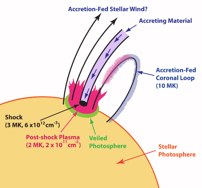
Romanova et al.  (2004) have used three-dimensional magnetohydrodynamic (MHD) simulations to show that the hot spots formed on the surface by accretion are inhomogeneous, with the lower density and temperature regions filling a larger surface area than the denser central region, seemingly suggestive of Region 2. However, the larger mass of Region 2 also implies a higher accretion rate than for Region 1, and thus a larger density, in contradiction to our diagnostics. Therefore, we do not interpret Region 2 as a second accretion shock with a different accretion rate, but rather as a new accretion-driven phenomena. The impact from the accretion presumably provides the energy to heat additional material in the stellar atmosphere to over 1 MK. Very recently, two-dimensional MHD simulations have shown that violent outflows of shock-heated material can propagate from the base of the accretion shock for cases with a high thermal to magnetic pressure ratio $\beta$ (Orlando et al.  2009).

One of the key concepts of the standard one-dimensional accretion model suggests a simple picture (Fig. 10). The field line that truncates the disk separates the open magnetic field lines of the polar region from the closed magnetic field loops in the equatorial regions. The region heated by the shock (our Region 2) provides a large supply of ionized material available to form the soft X-ray emitting corona presented here, a warm wind (Dupree et al.  2005), and soft X-ray jets (Güdel et al.  2008). This corona exists because magnetic loops confine it, but it is fed by the accretion process and is thus unlike stellar coronae in dwarf stars on the main sequence. Figure 10 illustrates the shock and its surroundings.

Figure 10.— Illustration of the shock and its surrounding environment. Region 1 in the text corresponds to the shock and Region 2 to the postshock plasma. Figure courtesy of A.  Szentgyorgyi.

This model provides an explanation for the soft X-ray excess discovered in the XMM-Newton Extended Survey of the Taurus Molecular Cloud (XEST; Güdel et al.  2007c; Telleschi et al.  2007). Grating spectra show that this excess emission manifests itself in CTTS as enhanced O VII relative to O VIII as compared with weak-line T Tauri (WTTS) and main-sequence stars (Güdel & Telleschi 2007; Robrade & Schmitt 2007). Our O VII measurements also demonstrate that the postshock cooling gas can, in some cases, dilute the signature of high $N_{e}$ and explain why not all accreting systems show high densities.

Having carefully distinguished between the accretion and corona in Section 3, we reconsider the assumption that these two components arise from different processes. Güdel & Telleschi (2007) find that the soft X-ray excess depends both on the level of magnetic activity as measured by the total (including coronal) $L_{X}$ and on the presence of accretion. While we suggest that the role of accretion is to heat and ionize the surrounding stellar atmosphere to create a soft X-ray (postshock cooling) plasma, it seems possible that this plasma could be further heated to $\sim 10$ MK, either by the usual coronal heating (MHD) processes, or possibly by the accretion energy. Cranmer (2009) finds that in some systems, accretion can provide the energy for coronal heating to such high temperatures.

Studies of star forming regions have found that young stars show strong X-ray activity, with energetic flares and extremely high X-ray emitting temperatures; however, the increase in activity with rotation rate breaks down for the accreting systems, leading to the conjecture that the stellar dynamo might operate differently in these systems (Preibisch et al.  2005). We suggest that the accretion process may play a more prominent role than has generally been believed. While X-ray signatures of the accretion shock itself may not usually dominate the emission, the energy from accretion may in fact contribute to feeding and heating a new type of corona.

6. Summary and Conclusions

We have analyzed the deep Chandra HETG spectrum of TW Hya to assess the relative contributions of accretion and coronal emission. We summarize the most important of our findings:

• The spectrum shows line and continuum emission from $\sim 10$ MK coronal plasma, which may have a broad emission measure distribution. Unlike active main sequence stars, the coronal EM distribution abruptly cuts off below $\sim 5$ MK, probably due to absorption by the accretion stream.

• The spectrum also shows emission lines from plasma at $T_{e}=2.5$ MK, as predicted by standard models of the accretion shock. $T_{e}$ and $N_{e}$ diagnostics from He-like Ne IX are in excellent agreement with accretion models for TW Hya.

• We measure the flux of the O VII forbidden line in TW Hya for the first time to better than 3$\sigma$, allowing a determination of electron density. This density is lower than $N_{e}$ from Ne IX by a factor of four and lower than $N_{e}$ from the standard postshock cooling model by a factor of seven, and leads to a new model of an accretion-fed corona.

• The high $T_{e}$ ions suggest a stellar corona. By contrast, line ratio diagnostics from the lower $T_{e}$ ions, indicate two regions with different densities. In our model, the accretion shock itself has $T_{e}=3.0$ MK and $N_{e}=6.0\times 10^{12}$ cm^-3, while the postshock cooling region has $T_{e}=1.75$ MK and $N_{e}=2.0\times 10^{11}$ cm^-3. The postshock plasma has 30 times more mass than the shock itself. The surface area filling factor of the shock is 1.5% while the postshock filling factor is approximately 6.8%.

• Line ratio diagnostics require at least two different absorbers, with higher column density ($N_{H}$) for higher charge state. Absorption by the accretion stream is larger by a factor of 2.5 for the shock than for the postshock region.

• A range of models for the EM distribution and elemental abundances provides acceptable fits to the global spectrum. While absorption, emission measure, and abundances are not independently determined by such methods, the high Ne/O abundance seems to be a robust result.

• From line profile analysis of Ne IX lines we determine a subsonic turbulent velocity of about 165 km s^-1.

This high resolution X-ray spectrum of TW Hya presents a rich set of diagnostic emission lines for characterizing the physical conditions of the high energy plasma and understanding the dominant physical processes. The observations strongly support the model of an accretion shock producing a few MK gas at high density, as first suggested by Kastner et al.  (2002) from an earlier HETG spectrum. The diagnostics also support the role of accretion in producing the soft X-ray excess at O VII previously discovered (Güdel & Telleschi 2007; Robrade & Schmitt 2007). This excess emission requires that the accretion shock heat a large volume in the surrounding stellar atmosphere. In TW Hya the filling factor at O VII is larger than the filling factor of the shock at Ne IX, and is consistent with the filling factors of the ultraviolet and optical continua. Both open and closed magnetic field lines may emerge from this surrounding area to channel this ionized gas back into the corona. While it is not yet clear whether the energy from the impact of accretion at the star can heat a hot (10 MK) corona, accelerate a highly ionized stellar wind, or drive hot jets, we suggest that accretion-fed coronae may be ubiquitous in accreting young stars.

References

- A (1999) Anders, E., & Grevesse, N. 1989, Geochim. Cosmochim. Acta, 53, 197
- A (1999) Argiroffi, C., Maggio, A., & Peres, G. 2007, A&A, 465, L5
- A (1999) Argiroffi, C., Maggio, A., & Peres, G., Drake, J. J., Lopez Santiago, J., Sciortino, S., & Stelzer, B. 2009, A&A, accepted (arXiV: 0909.0218)
- A (1999) Batalha, C., Batalha, N. M., Alencar, S. H. P., Lopes, D. F., & Duarte, E. S. 2002, ApJ, 580, 343
- A (1999) Brown, G. V., Beiersdorfer, P., Chen, H., Chen, M. H., & Reed, K. J. 2001, ApJ, 557, L75
- A (1999) Calvet, N., & Gullbring, E. 1998, ApJ, 509, 802
- A (1999) Calvet, N., D’Alessio, P., Hartmann, L., Wilner, D., Walsh, A., & Sitko, M. 2002, ApJ, 568, 1008
- A (1999) Chen, G.-X., Smith, R. K., Kirby, K. P., Brickhouse, N. S., & Wargelin, B. J. 2006, PRA, 74, 2709
- A (1999) Costa, V. M., Lago, M. T. V. T., Norci, L., & Meurs, E. J. A. 2000, A&A, 354, 621
- A (1999) Cranmer, S. R. 2008, ApJ, 689, 316
- A (1999) Cranmer, S. R. 2009, ApJ, 706, 824
- A (1999) Drake, J. J. 2005, in Proceedings of the 13th Workshop on Cool Stars, Stellar Systems, and the Sun, ESA SP-560, 519
- A (1999) Drake, J. J., Testa, P., & Hartmann, L. 2005, ApJ, 627, L149
- A (1999) Dupree, A. K., Brickhouse, N. S., Smith, G. H., & Strader, J. 2005, ApJ, 625, L131
- A (1999) Favata, F., Flaccomio, E., Reale, F., Micela, G., Sciortino, S., Shang, H., Stassun, K. G., & Feigelson, E. D. 2005, ApJS, 160, 469
- A (1999) Feigelson, E. D., & Montmerle, T. 1999, ARA&A, 37, 363
- A (1999) Feldmeier, A., Kudritzki, R.-P., Palsa, R., Pauldrach, A. W. A., & Puls, J. 1997, A&A, 320, 899
- A (1999) Freeman, P. E., Doe, S., & Siemiginowska, A. 2001, SPIE Proceedings, 4477, 76
- A (1999) Fruscione, A. et al. 2006, SPIE Proceedings, 6270, 60
- A (1999) Gagné, M., Skinner, S. L., & Daniel, K. J. 2004, ApJ, 613, 393
- A (1999) Gregory, S. G., Wood, K., & Jardine, M. 2007, MNRAS, 379, L35
- A (1999) Güdel, M., Skinner, S. L., Mel’Nikov, S. Yu, Audard, M., Telleschi, A., Briggs, & K. R. 2007a, A&A, 468, 529
- A (1999) Güdel, M., Telleschi, A., Audard, M., Skinner, S. L., Briggs, K. R., Palla, F., & Dougados, C. 2007b, A&A, 468, 515
- A (1999) Güdel, M. et al. 2007c, A&A, 468, 353
- A (1999) Güdel, M., & Telleschi, A. 2007 A&A, 474, L25
- A (1999) Güdel, M., Skinner, S. L., Audard, M., Briggs, K. R., & Cabrit, S. 2008, A&A, 478, 797
- A (1999) Günther, H. M., Liefke, C., Schmitt, J. H. M. M., Robrade, J., & Ness, J.-U. 2006, A&A, 459, L29
- A (1999) Günther, H. M., Schmitt, J. H. M. M., Robrade, J., & Liefke, C. 2007, A&A, 466, 1111
- A (1999) Hartmann, L. 1998, Accretion Processes in Star Formation, (Cambridge U. Press)
- A (1999) Hartmann, L., Cassen, P., & Kenyon, S. J. 1997, ApJ, 475, 770
- A (1999) Herczeg, G. J., Linsky, J. L., Valenti, J. A., Johns-Krull, C. M., & Wood, B. E. 2002, ApJ, 572, 310
- A (1999) Herczeg, G. J., Wood, B. E., Linsky, J. L., Valenti, J. A., & Johns-Krull, C. M. 2004, ApJ, 607, 369
- A (1999) Huenemoerder, D. P., Canizares, C. R., & Schulz, N. S. 2001, ApJ, 559, 1135
- A (1999) Huenemoerder, D. P., Kastner, J. H., Testa, P., Schulz, N. S., & Weintraub, D. A. 2007, ApJ, 671, 592
- A (1999) Kastner, J. H., Huenemoerder, D. P., Schulz, N. S., & Weintraub, D. A. 1999, ApJ, 525, 837
- A (1999) Kastner, J. H., Huenemoerder, D. P., Schulz, N. S., Canizares, C. R., & Weintraub, D. A. 2002, ApJ, 567, 434; K02
- A (1999) Königl, A. 1991, ApJ, 370, L39
- A (1999) Lamzin, S. A. 1999, Astron Lett, 25, 430
- A (1999) Mauche, C. W., Liedahl, D. A., & Fournier, K. B. 2001, ApJ, 560, 992
- A (1999) Morrison, R., & McCammon, D. 1983, ApJ, 270, 119
- A (1999) Muzerolle, J., Calvet, N., Briceño, C., Hartmann, L., & Hillenbrand, L. 2000, ApJ, 535, L47
- A (1999) Muzerolle, J., Calvet, N., & Hartmann, L. 2001, ApJ, 550, 944
- A (1999) Ness, J.-U., Schmitt, J. H. M. M., Burwitz, V., Mewe, R., Raassen, A. J. J., van der Meer, R. L. J., Predehl, P., & Brinkman, A. C. 2002, A&A, 394, 911
- A (1999) Ness, J.-U., Brickhouse, N. S., Drake, J. J., & Huenemoerder, D. P. 2003, ApJ, 598, 1277
- A (1999) Ness, J.-U., Güdel, M., Schmitt, J. H. M. M., Audard, M., & Telleschi, A. 2004, A&A, 427, 667
- A (1999) Ness, J.-U., & Schmitt, J. H. M. M. 2005, A&A, 444, L41
- A (1999) Orlando, S., Sacco, G. G., Argiroffi, C., Reale, F., Peres, G., & Maggio, A. 2009, A&A, accepted (arXiv:0912.1799)
- A (1999) Osten, R. A., Ayres, T. R., Brown, A., Linsky, J. L., & Krishnamurthi, A. 2003, ApJ, 582, 1073
- A (1999) Porquet, D., Mewe, R., Dubau, J., Raassen, A. J. J., & Kaastra, J. S. 2001, A&A, 376, 1113
- A (1999) Preibisch, T. et al. 2005, ApJS, 160, 401
- A (1999) Qi, C. et al. 2004, ApJ, 616, L11
- A (1999) Raassen, A. J. J. 2009, A&A, 505, 755
- A (1999) Raymond, J. C. 1988, in Hot Thin Plasmas in Astrophysics, ed. R. Pallavicini, (Dordrecht: Kluwer), 3
- A (1999) Robrade, J., & Schmitt, J. H. M. M. 2007, A&A, 473, 229
- A (1999) Romanova, M. M., Ustyugova, G. V., Koldoba, A. V., & Lovelace, R. V. E. 2004, ApJ, 610, 920
- A (1999) Sanz-Forcada, J., Brickhouse, N. S., & Dupree, A. K. 2003, ApJS, 145, 147
- A (1999) Schmitt, J. H. M. M., Robrade, J., Ness, J.-U., Favata, F., & Stelzer, B. 2005, A&A, 432, L35
- A (1999) Schneider, P. C. & Schmitt, J. H. M. M. 2008, A&A, 488, L13
- A (1999) Smith, R. K., Brickhouse, N. S., Liedahl, D. A., & Raymond, J. C. 2001, ApJ, 556, L91
- A (1999) Smith, R. K., Chen, G.-X., Kirby, K. P., & Brickhouse, N. S. 2009a, ApJ, 700, 679
- A (1999) Smith, R. K., Chen, G.-X., Kirby, K. P., & Brickhouse, N. S. 2009b, ApJ, 701, 203
- A (1999) Stelzer, B., & Schmitt, J. H. M. M. 2004, A&A, 418, 687
- A (1999) Telleschi, A., Güdel, M., Briggs, K. R., Audard, M., & Scelsi, L. 2007, A&A, 468, 443
- A (1999) Testa, P., Drake, J. J., & Peres, G. 2004, ApJ, 617, 508