A note on the group lasso and a sparse group lasso

Abstract

We consider the group lasso penalty for the linear model. We note that the standard algorithm for solving the problem assumes that the model matrices in each group are orthonormal. Here we consider a more general penalty that blends the lasso ($L_{1}$) with the group lasso (“two-norm”). This penalty yields solutions that are sparse at both the group and individual feature levels. We derive an efficient algorithm for the resulting convex problem based on coordinate descent. This algorithm can also be used to solve the general form of the group lasso, with non-orthonormal model matrices.

1 Introduction

In this note, we consider the problem of prediction using a linear model. Our data consist of $\bf y$, a vector of $N$ observations, and $\bf X$, a $N\times p$ matrix of features.

Suppose that the $p$ predictors are divided into $L$ groups, with $p_{\ell}$ the number in group $\ell$. For ease of notation, we use a matrix ${\bf X}_{\ell}$ to represent the predictors corresponding to the $\ell$th group, with corresponding coefficient vector $\beta_{\ell}$. Assume that $\bf y$ and ${\bf X}$ has been centered, that is, all variables have mean zero.

In an elegant paper, YL2007 proposed the group lasso which solves the convex optimization problem

$$\min_{\beta\in{\rm R}^{p}}\left(||{\bf y}-{\bf 1}-\sum_{\ell=1}^{L}{\bf X}_{\ell}\beta_{\ell}||_{2}^{2}+\lambda\sum_{\ell=1}^{L}\sqrt{p_{\ell}}||\beta_{\ell}||_{2}\right),$$ (1)

where the $\sqrt{p_{\ell}}$ terms accounts for the varying group sizes, and $||\cdot||_{2}$ is the Euclidean norm (not squared). This procedure acts like the lasso at the group level: depending on $\lambda$, an entire group of predictors may drop out of the model. In fact if the group sizes are all one, it reduces to the lasso. meier2008 extend the group lasso to logistic regression.

The group lasso does not, however, yield sparsity within a group. That is, if a group of parameters is non-zero, they will all be non-zero. In this note we propose a more general penalty that yields sparsity at both the group and individual feature levels, in order to select groups and predictors within a group. We also point out that the algorithm proposed by YL2007 for fitting the group lasso assumes that the model matrices in each group are orthonormal. The algorithm that we provide for our more general criterion also works for the standard group lasso with non-orthonormal model matrices.

We consider the sparse group lasso criterion

$$\min_{\beta\in{\rm R}^{p}}\left(||{\bf y}-\sum_{\ell=1}^{L}{\bf X}_{\ell}\beta_{\ell}||_{2}^{2}+\lambda_{1}\sum_{\ell=1}^{L}||\beta_{\ell}||_{2}+\lambda_{2}||\beta||_{1}\right).$$ (2)

where $\beta=(\beta_{1},\beta_{2},\ldots\beta_{\ell})$ is the entire parameter vector. For notational simplicity we omit the weights $\sqrt{p_{\ell}}$. Expression (2) is the sum of convex functions and is therefore convex. Figure 1 shows the constraint region for the group lasso, lasso and sparse group lasso.

Figure 1: Contour lines for the penalty for the group lasso (dotted), lasso (dashed) and sparse group lasso penalty (solid), for a single group with two predictors.

A similar penalty involving both group lasso and lasso terms is discussed in peng2009. When $\lambda_{2}=0$, criterion (2) reduces to the group lasso, whose computation we discuss next.

2 Computation for the group lasso

Here we briefly review the computation for the group lasso of YL2007. In the process we clarify a confusing issue regarding orthonormality of predictors within a group.

The subgradient equations (see e.g. Bertsekas1999) for the group lasso are

$$-{\bf X}_{\ell}^{T}(y-\sum_{\ell}{\bf X}_{\ell}\beta_{\ell})+\lambda\cdot s_{\ell}=0;\;\ell=1,2,\ldots L,$$ (3)

where $s_{\ell}=\beta_{\ell}/||\beta_{\ell}||$ if $\beta_{\ell}\neq 0$ and $s_{\ell}$ is a vector with $||s_{\ell}||_{2}<1$ otherwise. Let the solutions be $\hat{\beta}_{1},\hat{\beta}_{2}\ldots\hat{\beta}_{\ell}$. If

$$||{\bf X}_{\ell}^{T}(y-\sum_{k\neq\ell}{\bf X}_{k}\hat{\beta}_{k})||<\lambda$$ (4)

then $\hat{\beta}_{\ell}$ is zero; otherwise it satisfies

$$\hat{\beta}_{\ell}=({\bf X}_{\ell}^{T}{\bf X}_{\ell}+\lambda/||\hat{\beta}_{\ell}||)^{-1}{\bf X}_{\ell}^{T}r_{\ell}$$ (5)

where

$${\bf r}_{\ell}={\bf y}-\sum_{k\neq\ell}{\bf X}_{k}\hat{\beta}_{k}$$

Now if we assume that ${\bf X}_{\ell}^{T}{\bf X}_{\ell}={\bf I}$, and let $s_{\ell}={\bf X}_{\ell}^{T}r_{\ell}$, then (5) simplifies to $\hat{\beta}_{\ell}=(1-\lambda/||s_{\ell}||)s_{\ell}$. This leads to an algorithm that cycles through the groups $k$, and is a blockwise coordinate descent procedure. It is given in YL2007.

If however the predictors are not orthonormal, one approach is to orthonormalize them before applying the group lasso. However this will not generally provide a solution to the original problem. In detail, if ${\bf X}_{\ell}={\bf U}{\bf D}{\bf V}^{T}$, then the columns of ${\bf U}={\bf X}_{\ell}{\bf V}{\bf D}^{-1}$ are orthonormal. Then ${\bf X}_{\ell}{\bf\beta}_{\ell}={\bf U}{\bf V}{\bf D}^{-1}{\bf\beta}_{\ell}={\bf U}[{\bf V}{\bf D}^{-1}{\bf\beta}_{\ell}]={\bf U}{\bf\beta}_{\ell}*$. But $||{\bf\beta}_{\ell}*||=||{\bf\beta}_{\ell}||$ only if ${\bf D}={\bf I}$. This will not be true in general, e.g. if ${\bf X}$ is a set of dummy varables for a factor, this is true only if the number of observations in each category is equal.

Hence an alternative approach is needed. In the non-orthonormal case, we can think of equation (5) as a ridge regression, with the ridge parameter depending on $||\hat{\beta}_{\ell}||$. A complicated scalar equation can be derived for $||\hat{\beta}_{\ell}||$ from (5); then substituting into the right-hand side of (5) gives the solution. However this is not a good approach numerically, as it can involve dividing by the norm of a vector that is very close to zero. It is also not guaranteed to converge. In the next section we provide a better solution to this problem, and to the sparse group lasso.

3 Computation for the sparse group lasso

The criterion (1) is separable so that block coordinate descent can be used for its optimization. Therefore we focus on just one group $\ell$, and denote the predictors by ${\bf X}_{\ell}=Z=(Z_{1},Z_{2},\ldots Z_{k})$, the coefficients by $\beta_{\ell}={\bf\theta}=(\theta_{1},\theta_{2},\ldots\theta_{k})$ and the residual by ${\bf r}={\bf y}-\sum_{k\neq\ell}X_{k}\beta_{k}$. The subgradient equations are

$$-Z_{j}^{T}({\bf r}-\sum_{j}Z_{j}\theta_{j})+\lambda_{1}s_{j}+\lambda_{2}t_{j}=0$$ (6)

for $j=1,2,\ldots k$ where $s_{j}=\theta_{j}/||{\bf\theta}||$ if ${\bf\theta}_{\ell}\neq 0$ and $s$ is a vector satisfying $||s||_{2}\leq 1$ otherwise, and $t_{j}\in{\rm sign(\theta_{j})}$, that is $t_{j}=sign(\theta_{j})$ if $\theta_{j}\neq 0$ and $t_{j}\in[-1,1]$ if $\theta_{j}=0$. Letting ${\bf a}={\bf X}_{\ell}{\bf r}$, then a necessary and sufficient condition for ${\bf\theta}$ to be zero is that the system of equations

$$a_{j}=\lambda_{1}s_{j}+\lambda_{2}t_{j}$$ (7)

have a solution with $||s||_{2}\leq 1$ and $t_{j}\in[-1,1]$. We can determine this by minimizing

$$J(t)=(1/\lambda_{1}^{2})\sum_{j=1}^{k}(a_{j}-\lambda_{2}t_{j})^{2}=\sum_{j=1}^{k}s_{j}^{2}$$ (8)

with respect to the $t_{j}\in[-1,1]$ and then checking if $J(\hat{t})\leq 1$. The minimizer is easily seen to be

$$\hat{t}_{j}=\begin{cases}\frac{a_{j}}{\lambda_{2}}&\text{if $|\frac{a_{j}}{\lambda_{2}}|\leq 1$,}\\ {\rm sign}(\frac{a_{j}}{\lambda_{2}})&\text{if $|\frac{a_{j}}{\lambda_{2}}|>1$.}\end{cases}$$

Now if $J(\hat{t})>1$, then we must minimize the criterion

$$\frac{1}{2}\sum_{i=1}^{N}\Bigl{(}r_{i}-\sum_{j=1}^{k}Z_{ij}\theta_{j}\Bigr{)}^{2}+\lambda_{1}||{\bf\theta}||_{2}+\lambda_{2}\sum_{j=1}^{k}|\theta_{j}|$$ (9)

This is the sum of a convex differentiable function (first two terms) and a separable penalty, and hence we can use coordinate descent to obtain the global minimum.

Here are the details of the coordinate descent procedure. For each $j$ let ${\bf r}_{j}={\bf r}-\sum_{k\neq j}Z_{k}\hat{\theta}_{k}$. Then $\hat{\theta}_{j}=0$ if $|Z_{j}^{T}{\bf r}_{j}|<\lambda_{2}$. This follows easily by examining the subgradient equation corresponding to (9). Otherwise if $|Z_{j}^{T}{\bf r}_{j}|\geq\lambda_{2}$ we minimize (9) by a one-dimensional search over $\theta_{j}$. We use the optimize function in the R package, which is a combination of golden section search and successive parabolic interpolation.

This leads to the following algorithm:

Algorithm for the sparse group lasso

1. Start with $\hat{\beta}=\beta_{0}$

2. In group $\ell$ define ${\bf r}_{\ell}={\bf y}-\sum_{k\neq\ell}{\bf X}_{k}\beta_{k}$, ${\bf X}_{\ell}=(Z_{1},Z_{2},\ldots Z_{k})$, $\beta_{\ell}=(\theta_{1},\theta_{2},\ldots\theta_{k}$) and ${\bf r}_{j}={\bf y}^{\prime}-\sum_{k\neq j}Z_{k}\theta_{k}$. Check if $J(\hat{t})\leq 1$ according to (8) and if so set $\hat{\beta}_{\ell}=0$. Otherwise for $j=1,2,\ldots k$, if $|Z_{j}^{T}{\bf r}_{j}|<\lambda_{2}$ then $\hat{\theta}_{j}=0$; if instead $|Z_{j}^{T}{\bf r}_{j}|\geq\lambda_{2}$ then minimize

   $$\frac{1}{2}\sum_{i=1}^{N}(y^{\prime}_{i}-\sum_{j=1}^{k}Z_{ij}\theta_{j})^{2}+\lambda_{1}||{\bf\theta}||_{2}+\lambda_{2}\sum_{j=1}^{k}|\theta_{j}|$$ (10)

   over $\theta_{j}$ by a one-dimensional optimization.

3. Iterate step (2) over groups $\ell=1,2,\ldots L$ until convergence.

If $\lambda_{2}$ is zero, we instead use condition (4) for the group-level test and we don’t need to check the condition $|Z_{j}^{T}{\bf r}_{j}|<\lambda_{2}$. With these modifications, this algorithm also gives a effective method for solving the group lasso with non-orthogonal model matrices.

Note that in the special case where ${\bf X}_{\ell}^{T}{\bf X}_{\ell}=I$, with ${\bf X}_{\ell}=(Z_{1},Z_{2},\ldots Z_{k})$ then its is easy to show that

$$\hat{\theta}_{j}=\Bigl{(}||S(Z_{j}^{T}{\bf y},\lambda_{2})||_{2}-\lambda_{1}\Bigr{)}_{+}\frac{S(Z_{j}^{T}{\bf y},\lambda_{2})}{||S(Z_{j}^{T}{\bf y},\lambda_{2})||_{2}}$$ (11)

and this reduces to the algorithm of YL2007.

4 An example

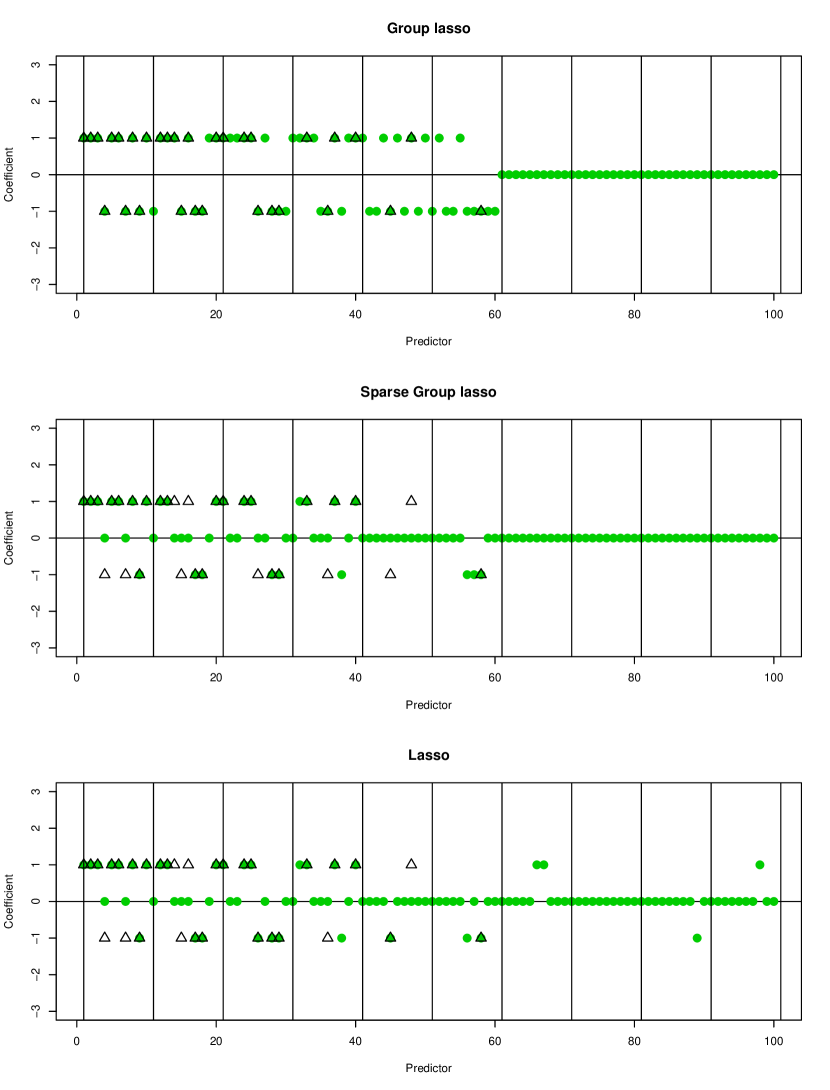
We generated $n=200$ observations with $p=100$ predictors, in ten blocks of ten. The second fifty predictors iall have coefficients of zero. The number of non-zero coefficients in the first five blocks of 10 are (10, 8, 6, 4, 2, 1) respectively, with coefficients equal to $\pm 1$, the sign chosen at random. The predictors are standard Gaussian with correlation 0.2 within a group and zero otherwise. Finally, Gaussian noise with standard deviation 4.0 was added to each observation.

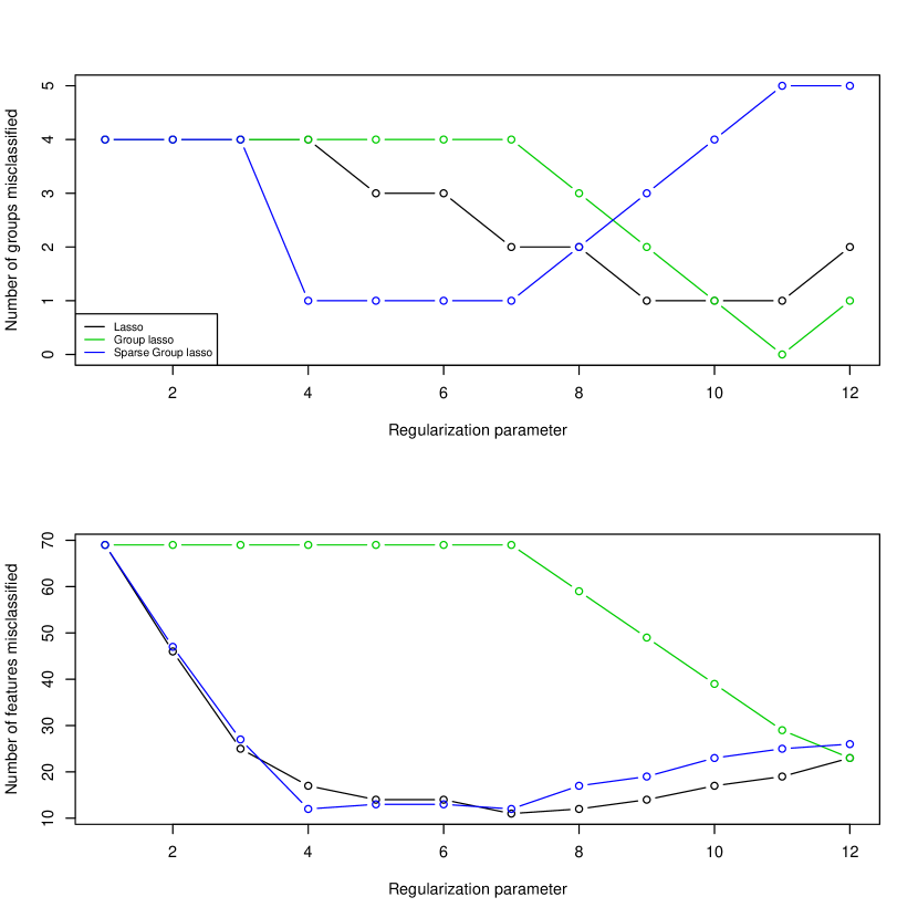
Figure 2 shows the signs of the estimated coefficients from the lasso, group lasso and sparse group lasso, using a well chosen tuning parameter for each method (we set $\lambda_{1}=\lambda_{2}$ for the sparse group lasso). The corresponding misclassification rates for the groups and individual features are shown in Figure 3. We see that the sparse group lasso strikes an effective compromise between the lasso and group lasso, yielding sparseness at the group and individual predictor levels.

Figure 2: Results for the simulated example. True coefficients are indicated by the open triangles while the filled green circles indicate the sign of the estimated coefficients from each method.

Figure 3: Results for the simulated example. The top panel shows the number of groups that are misclassified as the regularization parameter is varied. A misclassified group is one with at least one nonzero coefficient whose estimated coefficients are all set to zero, or vice versa. The bottom panel shows the number of individual coefficients that are misclassified, that is, estimated to be zero when the true coefficient is nonzero or vice-versa.