Edge-induced spin polarization in two-dimensional electron gas

Abstract

We characterize the role of the spin-orbit coupling between electrons and the confining potential of the edge in nonequilibrium 2D homogeneous electronic gas. We derive a simple analytical result for the magnitude of the current induced spin polarization at the edge and prove that it is independent of the details of the confinement edge potential and the electronic density within realistic values of the parameters of the considered models. While the amplitude of the spin accumulation is comparable to the experimental values of extrinsic spin Hall effect in similar samples, the spatial extent of edge induced effect is restricted to the distances of the order of Fermi wavelength ($\sim$ 10nm).

I Introduction

One of the exciting new discoveries in solid state physics in the last few years has been the experimental observation of the extrinsic spin Hall effectKato04 ; Sih05 ; Wunderlich05 ; Sih05b in GaAs heterostructures. The mechanism of this effect relies on the spin-orbit coupling between the spin of electrons with the perturbing potential of impurities. Another example of similar coupling is the Rashba-Bytchkov interaction in asymmetrically doped GaAs quantum wells containing two-dimensional electron gas (2DEG) where the coupled potential comes from the internal electrostatic electric field induced by the structural asymmetry of the well. In modeling both of these situations, the atomic potential of the ideal bulk semiconductor enters only through the renormalization of the effective mass and the spin-orbit interaction strength.

Interestingly, the Rashba-Bytchkov interaction has been also suggested as a source of spin Hall-like phenomenologySinova04 for a clean 2DEG. While the effect has been shown to disappear in extended 2D systems with arbitrarily weak disorderInoue04 ; Rashba04 , it is now known that finite size of the sample in combination with Rashba-Bytchkov coupling results in the transverse spin current and accumulation of opposite spin densities at the edges of the sampleNikolic05a ; Moca07 . Furthermore, it has been found that boundaries might directly influence the spin polarization due to the Rashba-Bytchov coupling either in very wide 2D electronic systems with an edgeUsaj05 ; Reynoso06 ; Zyuzin07 ; Teodorescu09 ; Sonin09c or narrow Rashba stripsYao06 ; Li08 . However, the physical origin of the latter is quite different from the former: whereas the bulk Rashba-Bytchkov effect arises from accelerations of electrons in the external electric field, the latter result from the reflection of electrons from the sample’s boundary.

Motivated by this development, it is natural to explore further alterations of the perfectly periodic bulk potential and its consequences on the spin polarization in the presence of the current. Several authors have considered such a situation in quantum wires with a parabolic confining potentialBellucci06 ; Hattori06 ; Xing06 ; Bellucci07 , wider strips with parabolicJiang06 or abruptBokes08 confinement edge. These alterations in the potential landscape can be also viewed as the “impurity” which leads to nonzero spin polarization induced by the flow of the electric current. Recently, experimental evidence of this effect of the in-plane field on spin polarization has been reportedDebray09 . Further enhancement of this kind of spin-polarization has been suggested using a transport through chaotic quantum dotKrich08 or resonant tunable scattering centerYokoyama09 .

In our previous workBokes08 we have compared the magnitude of the spin polarization induced by the latter mechanism with the one induced by the Rashba-Bytchkov coupling and scattering of the edgeZyuzin07 . It turns out that for a typical 2DEG with an edge, it is about three orders of magnitude larger than the one caused by the edge and the Rashba-Bytchkov interaction. This substantial difference is mostly due to the fact that the parameter characterizing spin-orbit coupling appears in second order in the case of the Rashba-Bytchov-based mechanismZyuzin07 whereas for the edge-induced spin-orbit coupling it comes already in the first order.

In this paper we consider the edge of the 2DEG in Si doped GaAs quantum well, a system for which the spin Hall effect has been experimentally observed. This allows us to estimate the values of all the parameters entering and we can compare the importance of this edge-effect to the contribution of other mechanisms leading to current-induced spin polarization. The models considered here are reasonably realistic yet simple enough to be solved almost analytically. We derive a generally valid simple analytical formula for the induced number of electrons with un-compensated spin per unit length of the edge,

$$m_{z}=-\frac{m_{e}}{\hbar q_{e}}\alpha_{E}j,$$ (1)

where $j$ is the electrical current density in the 2DEG, $\alpha_{E}$ is the parameter giving the strength of the spin-orbit coupling Engel05 , and $m_{e}$ and $q_{e}$ are the effective mass and the charge of electron respectively. Noticeably, this result is independent of the density of the 2DEG and the details of the edge potential as long as the electrons are confined within the sample.

II The model of the edge and spin-orbit coupling

Let us consider a sample with 2DEG created within a GaAs-based quantum well. The electrical current in the plane of the 2DEG will be driven along the $y$ direction. We will be interested in the physics close to one of the two edges of the sample along which the current flows. The coordinate in the direction perpendicular to the edge will be $x$, $x>0$ corresponding to the region where the 2DEG is present (see Fig. 1).

We will describe the electronic states for electrons in the 2DEG within the effective mass approximation, treating the electrons as noninteracting quasiparticles. Qualitative changes in our results introduced within a self-consistent mean-field treatment will be studied afterwards. The length scale characterizing the electrons is given by their Fermi wavelength. It typically attains values $\lambda_{F}=\sqrt{2\pi/n_{2D}}\sim 2.5a_{B}^{*}$, where $n_{2D}$ is the two-dimensional electronic density and $a_{B}^{*}=9.79$nm is the effective Bohr radius in GaAs. Since this is about two orders of magnitude larger than the inter-atomic distances, we can employ the effective mass theory and approximate the form of the confining potential with a simple functional form.

In our work will assume that the confining edge potential, $V(x)$, is independent of the coordinate $y$, directed along the edge. Within our analytical derivations we model $V(x)$ as an abrupt step of height $\Delta V$, $V(x)=V_{\theta}(x)=\Delta V\theta(-x)$, where $\theta(x)$ is the unit step function. The actual value of the step is much larger than the Fermi energy of the 2DEG. This is frequently used to set the potential step to infinity. However, here it is essential that the step is finite as the whole spin-orbit coupling is nonzero only in the region of the nonzero gradient of the confining potential. Since this value should be of the order of the work function of the electrons in the 2DEG, we fix this value to $\Delta V=2.7$eV$\sim 230$Ha^∗. One of the results of our work is the demonstration that the current induced spin polarization is rather independent of this value so that we do not need to be concerned with its precise numerical value, as long as it is large ($>>E_{F}$) but finite value.

Once we establish the analytical result for this model of abrupt potential step, we will also consider more general forms: step with a linear slope on a distance $d$, $V_{d}(x)$ (used in Fig. 1), and a partially self-consistent, density-dependent model with a small triangular-shaped dip, $V_{n}(x)$, close to the edge. In the absence of this dip, the decrease in the density to zero at the edge in the 2DEG results in a slight local depletion of electrons there. A small negative value of the depth of the dip, $-V_{0}$, that is found self-consistently results in a charge neutral edge which is the physically expected situation.

The essential part of our model is the spin-orbit (SO) coupling term in the electrons’ Hamiltonian. In general, several different types of SO interactions can be similar in magnitude: the Rashba-Bytchkov, the Dresselhaus or the impurity-induced SO coupling. However, since they are all small perturbations to the effective Hamiltonian, we can consider them separably and superpose their outcomes in the sense of first order perturbation theory in terms of SO parameter appearing in the SO interaction. In our paper we will consider a special case of the impurity-induced SO coupling for the special case when the “impurity” is the edge potential only. In general, the SO contribution to the Hamiltonian takes the formWinklerBook

$$\hat{V}^{SO}=\alpha_{E}\vec{\sigma}\cdot\left(\vec{k}\times\nabla V(x)\right),$$ (2)

where $\alpha_{E}$ characterizes the strength of the SO coupling, $\vec{\sigma}$ are Pauli matrices, $\vec{k}$ is the operator of electron’s momentum and $V(x)$ is the effective one-electron potential energy. Within our study the latter corresponds to various models of the edge potential: $V_{\theta}(x)$, $V_{d}(x)$ or $V_{n}(x)$. The strength of the SO coupling in GaAs is known to be approximately $\alpha_{E}\approx 5.3\AA^{2}=5.53\times 10^{-4}$a${}_{B}^{*}$ which is $10^{6}$ times larger than the strength of the SO coupling in vacuumEngel05 .

Within the framework of this model it is very easy to understand the origin of the current-induced spin polarization. The gradient of the potential energy is directed only in the $x$ direction, the momentum is confined only within the $xy$ plane so that the only nonzero component of the spin operator comes from its $z$ component due to the mixed product form in Eq. 2. Specifically, the SO interaction is simply a spin-dependent potential

$$\hat{V}^{SO}=-\alpha_{E}\sigma_{z}qV^{\prime}(x)$$ (3)

with a well defined quantum number for the projection of the spin in the $z$ direction, $\sigma_{z}$, attaining values $\pm 1$, and $q$ is the $y$ component of the electron’s momentum (Fig. 1). Hence, the spin-orbit term is a potential energy which, for states with positive momentum in the $+y$ direction (the current), is smaller (larger) in the spatial region of negative derivative of the edge potential, $V^{\prime}(x)<0$, for electrons with their spin down (up). Since close to $x=0$ we have $V^{\prime}(x)=-\Delta V\delta(x)<0$, we expect that close to the edge we will find majority of spin-down electrons. Of course, in equilibrium for zero total current density there will be equal number of electron with $q>0$ and $q<0$ so that in this special case zero total spin polarization will be observed.

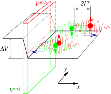
Figure 1: (Color online) The edge’s confinement potential of depth $\Delta V$ leads, via the SO coupling (Eq. 3) to attractive potential ($V^{SO,\downarrow}$, in green) for electrons with spin down in the vicinity of the edge. The initially compensated spins of electrons approaching the edge becomes locally un-compensated due to the difference in the scattering shift $l^{a}$.

III Spin polarization and the spin-dependent phase-shift

In our previous work Bokes08 , we have given estimates for the total induced spin per unit length of the edge using arguments based on wavepacket propagation. We considered a single-electron wavepacket state, $\psi^{q,\sigma}_{k,\Delta k}(t)$, for a specific momentum in the $y$ direction $q$, spin $\sigma$, with momentum $k$ of uncertainty $\Delta k$,

$$\psi^{q,\sigma}_{k,\Delta k}(t) = \int_{k-\Delta k/2}^{k+\Delta k/2}\frac{dk}{\sqrt{2\pi\Delta k}}\left(e^{-ikx}+r^{q,\sigma}(k)e^{ikx}e^{iqy}\right)$$ (4)

$$\times e^{-i(k^{2}/2+q^{2}/2)t},$$

where $r^{q,\sigma}(k)$ is the reflection amplitude of the eigenstate with energy $E=(1/2)(k^{2}+q^{2})$. For large negative times only the incoming part (moving from the right in the Fig. 1) of this wavepacket will give rise to nonzero contributions (the reflected part will be extremely small due to the quickly oscillating factors) and the wavepacket will be approaching the edge (Fig. 1, moving to the left). On the other hand, for large positive times only the reflected wave will give nonzero contribution. The position and form of the reflected wavepacket will depend on the spin of the incoming wavepacket since the reflection amplitude, $r^{q,\sigma}(k)$ will be different for the two possible spin orientations. Specifically, it is shown in the Appendix A that the reflection amplitude has the form $r^{q,\sigma}(k)=e^{i\theta^{q,\sigma}_{k}}$ where the phase shift up to 3rd order in $\alpha_{E}$ is

$$\theta^{q,\uparrow/\downarrow}_{k} = \pi+2\textrm{atan}\frac{k}{\kappa}\mp 2k\alpha_{E}q+2k\kappa\alpha_{E}^{2}q^{2}$$ (5)

$$\mp 4\alpha_{E}^{3}q^{3}k(\Delta V-\frac{2}{3}k^{2}),$$

where $\kappa=\sqrt{2\Delta V-k^{2}}$. Assuming the width $\Delta k$ of the wavepacket $\psi^{q,\sigma}_{k,\Delta k}(t)$ small, one can easily find that the probability density of the reflected wavepackets with the phase-shift given by Eq. 5 for large times will take a form

$$|\psi^{q,\sigma}_{k,\Delta k}(t)|^{2}\approx\frac{1}{\pi}\frac{\sin^{2}\left(x(t)\Delta k/2\right)}{x(t)^{2}\Delta k/2}$$ (6)

where $x(t)=x+d\theta^{q,\sigma}/dk-kt$, i.e. the maximum of the probability is at $x=kt-d\theta^{q,\sigma}/dk$. From this it is evident that the electron with spin down will be lagging behind that with spin up by a distance $2l^{a}=d\theta^{q,\uparrow}/dk-d\theta^{q,\downarrow}/dk$ (indicated for the reflected right-going wavepackets in Fig. 1). This behavior of the scattering of single electron in the wavepacket can be directly extended to many-electrons in view of the stroboscopic wavepacket basisBokes08 . Namely, the above wavepackets for times $t_{m}=t+2\pi m/(k\Delta k)$, $m=0,\pm 1,\pm 2,...$, where $t$ is arbitrary moment of physical time, form orthogonal set of states which are all occupied with electrons. Hence the product of the length $2l^{a}$ times the number of electrons per area must give an estimate of the spin-polarization per unit length of the edge, as given in our previous work. Here we will show that this physically motivated estimate is in fact a rigorous result that we formally prove in the following, directly using the eigenstates of the Hamiltonian of the studied system.

The spin polarization per unit length of the edge is given in terms of the spin-resolved density as

$$m_{z}=\int_{-\infty}^{+\infty}dx\int\frac{dq}{2\pi}\int\frac{dk}{2\pi}(n^{k,q}_{\uparrow}(x)-n^{k,q}_{\downarrow}(x)),$$ (7)

where the integration in $q$ and $k$ goes over all the occupied eigenstates and $n^{k,q}_{\sigma}(x)$ is the contribution to the density at position $x,y$ from an occupied eigenstate

$$n^{k,q}_{\sigma}(x)=\left|e^{iqy}\left(e^{-ikx}+r^{q,\sigma}(k)e^{ikx}\right)\right|^{2}=2+2\Re\left\{e^{i(2kx+kl^{q,\sigma})}\right\}.$$ (8)

Since the spatial shift $l^{q,\sigma}$ is very small (given by the strength of the SO interaction), we can approximate the expression for the spin density to the first order

$$n^{k,q}_{\sigma}(x) = \left.n^{k,q}_{\sigma}(x)\right|_{l=0}+\left.\frac{d~{}}{dl}n^{k,q}_{\sigma}(x)\right|_{l=0}l^{q,\sigma},$$ (9)

$$= \left.n^{k,q}_{\sigma}(x)\right|_{l=0}+\left.\frac{1}{2}\frac{d~{}}{dx}n^{k,q}_{\sigma}(x)\right|_{l=0}l^{q,\sigma}$$ (10)

where we have interchanged the differentiation in view of the functional dependence of the density, Eq. 8 on $x$ and $l^{q,\sigma}$. Hence, using Eq. 7 and Eq. 10 we obtain for the spin polarization

$$m_{z} = \int\frac{dq}{2\pi}\int\frac{dk}{2\pi}\left.n^{k,q}_{\uparrow}(x)\right|_{x=-\infty}^{x=+\infty}l^{q}_{a},$$ (11)

where we have introduced the antisymmetric part of the spatial shift

$$l^{q}_{a}=\frac{\theta^{q,\uparrow}-\theta^{q,\downarrow}}{2k}=-2\alpha_{E}q-4\alpha_{E}^{3}q^{3}(\Delta V-\frac{2}{3}k^{2}).$$ (12)

The density at $x=-\infty$ is exponentially small, where as the contribution in the bulk of the 2DEG is according to Eq. 8 equal to $2$.

Including higher order terms in Eq. 10 would result in appearance of contributions with higher spatial derivatives of the density at $x=\pm\infty$. There, however, is the density constant (either zero for $x=-\infty$ or the homogeneous 2DEG value for $x=+\infty$) so that the expression for the spin polarization, Eq. 11 is correct also for large values of $l^{q,\sigma}$ in principle.

To complete the derivation we need to integrate over the occupied states. The simplest way is to assume that the non-equilibrium distribution is well described by a Fermi sphere with the radius (Fermi momentum) $k_{F}$ and the corresponding Fermi energy $E_{F}=k_{F}^{2}/2$ in 2D, shifted by a drift momentum $q_{d}$ in the $+y$ direction. Such a model corresponds to the distribution function maximizing the information entropy for a fixed average energy, density and current Bokes03 ; Bokes05 , and is also supported by Boltzmann-equation based analysis Rech09 . In the Appendix B we discuss the results obtained using the non-equilibrium model with two Fermi energies, conventional within the meso- and nano-scopic quantum transport. It gives identical result for the first order expansion in terms of $\alpha_{E}$; higher order terms in $\alpha_{E}$ differ by a numerical prefactor but are negligibly small for any realistic situations.

Using the expression for the asymmetric spatial shift, Eq. 12, we find for the induced spin polarization linear in the drift momentum (and hence the current density)

$$m_{z} = \int_{-k_{F}}^{k_{F}}\frac{dq}{2\pi}\int_{0}^{\sqrt{2E_{F}-q^{2}}}\frac{dk}{\pi}\left[l^{q+q_{d}}_{a}\right]$$ (13)

$$= \left(-\alpha_{E}-3\alpha_{E}^{3}\Delta VE_{F}+\frac{2}{3}\alpha_{E}^{3}E_{F}^{2}\right)q_{d}n_{2D}$$

where $k_{F}=\sqrt{2E_{F}}$ is the Fermi momentum, $n_{2D}=E_{F}/\pi$ is the density of the 2DEG. (See Fig. 5 for the explanation of the integration domain for $k,q$.) On the other hand, the current density is $j=q_{d}n_{2D}$ so that we find the final result

$$m_{z}=-\alpha_{E}j-3\alpha_{E}^{3}\Delta VE_{F}j+\frac{2}{3}\alpha_{E}^{3}E_{F}^{2}j+\mathcal{O}(\alpha_{E}^{5},j^{3})$$ (14)

In a typical situation, all except the first term of this expansion are negligibly small so that the resulting spin polarization is independent of the height of the confining potential $\Delta V$ and, according to the numerical results presented in the following section, practically independent of other gentle modifications of the model so that the first term should be useful as a general estimate of the magnitude of the current induced spin polarization in heterostructures based on 2DEG. Expressing the first order result in the S.I. units we obtain the central result of our work, stated in the introduction in Eq. 1.

IV Effects of the finite slope of the edge and the partial self-consistency

The aim of this section is to explore the rigidity of the result in Eq. 1 with respect to changes in the model of the confining potential at the edge. We will first address the dependence of our result on finite slope of the edge potential on the distance $d$ using the potential energy

$$V_{d}(x)=\left\{\begin{array}[]{cc}\Delta V&x<0\\ \Delta V-(\Delta V/d)x&0<x<d\\ 0&x>d\end{array}\right.$$ (15)

Qualitatively we can expect this dependence to be similarly weak as the dependence on $\Delta V$ obtained in the previous section (Eq. 14). The reason behind this is a mutual cancellation of two effects: (1) increasing $\Delta V$ increases the strength of the SO coupling in the Hamiltonian and hence the spin polarization, (2) increasing $\Delta V$ decreases the amplitude of the wavefunctions in the region of the nonzero gradient of the confining edge potential and hence its sensitivity to the SO coupling.

To characterize this dependence quantitatively we have evaluated the expression Eq. 7 numerically, where the spin-dependent contribution to the density, $n^{k,q}_{\sigma}(x)$, was obtained from the eigenfunctions of the effective 1D Hamiltonian containing the potential energy Eq. 15 and, according to Eq. 3, from it derived spin-orbit potential energy. The eigenfunctions were obtained by matching the plane-waves in regions $x<0$ and $x>d$ with the Airy functions in the region of the potential energy with linear slope, $0<x<d$. The integration over $k$ in Eq. 7 could be done analytically, whereas the integral over $q$ was done numerically on the regular mesh with $N_{k}$ points. We used model parameters that are typical for 2DEG created within GaAs quantum wells Sih05 , electronic density $n=0.985$ corresponding to the Fermi energy $E_{F}=3.01$, the current density $j=0.1$ and the value of the spin-orbit parameter $\alpha_{E}=5.53\times 10^{-4}$.

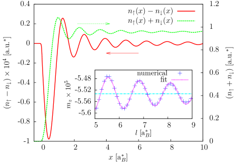
Figure 2: (Color online) The difference in spin densities (red-full) and the density (green-dashed) of electrons close to the edge of the sample (located at $x=0$). The former, similarly to the density, exhibits Friedel-like oscillations. Its first dominant local minimum (at $x\approx 0.2$) dominates the contribution to the nonzero spin-polarization obtained by integrating the difference in spin densities over whole $x$ axis. The inset demonstrates the extrapolation of this integration with respect to its upper limit, $l$, using a fit to a functional form $\sim A\sin(2k_{F}l+\phi)/l$.

For $d=0$ we confirm our analytical results for abrupt step potential, Eq. 14. The difference between the spin-up and spin-down densities, shown in Fig. 2, exhibits Friedel-like oscillations with the first period having a pronounced negative amplitude giving the major contribution to the non-zero spin polarization. The proportion of this amplitude to the electron is $\sim 10^{-4}$ for the current density $j=0.1$. Since the current density in the experimental situation is typically $j=0.1-0.01$ (the amplitude scales linearly with the current density for these values of $j$), this value is comparable to the amplitude of the spin polarization in the extrinsic spin Hall effectSih05b . Unfortunately, in contract to the extrinsic spin Hall effect, the nonzero spin-density is located only within few Fermi wavelengths away from the edge.

Integrating the difference in the spin densities along the whole $x$ axis we obtain the spin-polarization per unit length of the sample. The numerical result of this integration naturally depends on the upper limit of the integration; a reliable result, is easily obtained extrapolating the upper limit to infinity (inset of Fig. 2). Using this methodology we find the numerical result for the spin polarization $m_{z}=(5.53\pm 0.003)\times 10^{-5}$, which is in perfect agreement with our analytical expression, Eq. 14.

Using this extrapolation scheme we can address the changes in the spin-polarization with parameters of the model discussed in the following. First, we confirm the observation that the dependence on the magnitude of the confining edge potential comes in the 3rd order of $\alpha_{E}$: the value of the slope of the polarization vs. the height of the confinement edge potential, $\Delta V$ is $\partial m_{z}/\partial(\Delta V)\approx 1.6\times 10^{-10}$ which is close to the analytical value $1.5\times 10^{-10}$. The difference comes primarily from the extrapolation of the value of $m_{z}$ with respect to the upper limit of integration in $x$.

Considering nonzero values of the smearing length of the confining potential, $d\in(0,\lambda_{F}/2)$, we find that the resulting spin polarization is changing only very little ($\partial m_{z}/\partial d\sim 3.3\times 10^{-8}$). The reason for this negligible dependence is, similarly to the dependence on $\Delta V$, the mutual cancellation of the two effects discussed earlier.

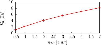
Figure 3: (Color online) The dependence of the self-consistent value of the potential dip $V_{0}$ on the electronic density shows monotonic behavior. While the value of the dip is comparable to the Fermi energy ($E_{F}=3.01$), the considered values do not lead to appearance of the bound state at the edge.

The second modification to the confining potential that we consider is partial self-consistency of the edge potential that guarantees charge neutrality of the edge of the sample. Presence of the model confining edge (Eq. 15) leads to redistribution of the charge density characterized with excess positive charge (per unit length of the sample)

$$\Delta N=\int_{-\infty}^{+\infty}dx\Delta n(x)=\int_{-\infty}^{+\infty}dx(E_{F}/\pi-n(x)),$$ (16)

where $n(x)$ is the electronic density and $E_{F}/\pi$ is the density of the positive background charge. The Fermi energy of the electrons guarantees that for large $x$ we have $n(x)=E_{F}/\pi$ so that the system is charge neutral in the bulk even through the total charge at the edge is not necessarily zero. The behavior of the density at the edge of a 2D sample is in contrast with the typical situation for the edge of 3D metals where the work function and the Fermi energy, mutually comparable in value, lead to leakage of the electronic density into vacuum and thereby to an access of negative charge LiebschBook . However at the edge of a 2DEG, the Fermi energy, typically few meV is much smaller than the work function which is of order of several eV and the situation is reversed.

The overall charge of the edge can be neutralized by a simple model potential

$$V_{n}(x)=\left\{\begin{array}[]{cc}\Delta V&x<0\\ -V_{0}+(2V_{0}/\lambda_{F})x&0<x<\lambda_{F}/2\\ 0&x>\lambda_{F}/2\end{array}\right.,$$ (17)

which on a distance $\lambda_{F}/2$ exhibits small potential dip to attract more electrons. The magnitude of the dip is obtained self-consistently to achieve zero total charge at the edge, i.e. the condition $\Delta N=0$. While in principle this form of the potential may support new bound states (edge states) for sufficiently large $V_{0}$, we have checked that for the here, self-consistently found values of $V_{0}$ no such states exist. The dependence of the self-consistent value of $V_{0}$ on the typical values of the density of the 2DEG is shown in Fig. 3.

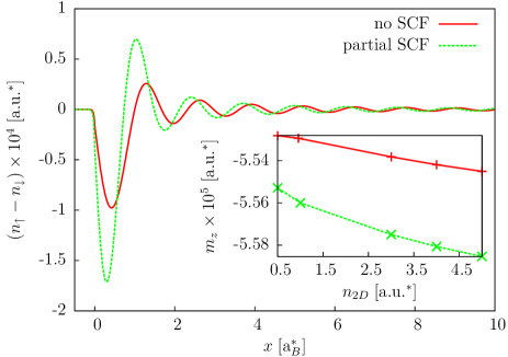
Figure 4: (Color online) The difference in the spin densities for non-interacting (red-full) and the partially self-consistent (green-dashed) electrons close to the edge of the sample (located at $x=0$). The spatially resolved spin density difference exhibits pronounced differences due to the selfconsistency, the most important effect being the shift of the curve closer to the edge. However, this results only in weak enhancement of the total spin polarization, $m_{z}$, shown in the inset for an interval of electronic densities, due to counter-acting spin-orbit coupling induced by the self-consistency correction in the region $x\in(0,\lambda_{F}/2)$.

Including the SO interaction, Eq. 3, on top of the potential energy $V_{n}(x)$, we obtain aditional repulsive SO-induced contribution for the spin-down electrons due to the linearly rising potential of the dip for $0<x<\lambda_{F}/2$. This is in competition with the character of the edge-confinement potential preferring the spin-down electrons. However, the dip in the potential energy also tends to move the electrons closer to the confining edge and, by increasing the density in this region, effectively enhances the effect of the SO coupling there. While the form of the spin-density does change significantly due to all these mechanisms (see Fig. 4), the overall spin polarization per unit length remains essentially unaltered over a wide range of electronic densities, shown in the inset of Fig. 4. This result once again confirms the rigidity of the result given by Eq. 1.

V Conclusions

The confining potential close to the edge of a 2D electron gas together with a nonzero current along this edge induces a nonzero spin polarization that is localized within a few Fermi wavelengths from the edge. To characterize this effect quantitatively we have derived a simple analytical formula for the spin polarization per unit length of the edge. Interestingly, the spin polarization is independent of the height of the confining potential as well as the electronic density of the 2DEG. Furthermore, using numerical calculations we have also showed that this result is independent on other possible modifications of the shape of the confining potential: the spatial extent of the confining potential and the partial selfconsistency of the confining potential with respect to charge neutrality of the edge.

VI Appendix A

The calculation of the spin-dependent phase-shift follows the usual textbook treatment of the wave-function matching method in 1D problems. For the separated $x-$ dependent factor of the eigenstate we need to solve the 1D Schrödinger equation

$$\left(-\frac{1}{2}\frac{d^{2}}{{dx}^{2}}+\Delta V\theta(-x)\pm\alpha_{E}q\Delta V\delta(x)\right)\phi^{q,\sigma}_{e}(x)=e\phi^{q,\sigma}_{e}(x),$$ (18)

where the ‘$+$’ sign is for $\sigma=\uparrow$ spin and the ’$-$’ sign for $\sigma=\downarrow$ spin. We are only interested in the solution well below the vacuum, i.e. $e<\Delta V$ for which we demand asymptotic forms

$$\phi^{q,\sigma}_{e}(x)=t^{q,\sigma}(\kappa)e^{\kappa x},\quad x<0,\kappa=\sqrt{2(\Delta V-e)}$$ (19)

$$\phi^{q,\sigma}_{e}(x)=e^{-ikx}+r^{q,\sigma}(k)e^{ikx},\quad x>0,k=\sqrt{2e}$$ (20)

The reflection amplitude ($r^{q,\sigma}(k)$) and the coefficient $t^{q,\sigma}(\kappa)$ are then found from the continuity of $\phi^{q,\sigma}_{e}(x)$ and its derivative at $x=0$ with the result

$$r^{q,\sigma}(k) = -\frac{\pm 2\alpha_{E}q\Delta V+\kappa+ik}{\pm 2\alpha_{E}q\Delta V+\kappa-ik}$$ (21)

$$t^{q,\sigma}(\kappa) = -\frac{2ik}{\pm 2\alpha_{E}q\Delta V+\kappa+ik}.$$ (22)

The sought phase shift is obtained from the reflection amplitude $r^{q,\sigma}_{e}=|r^{q,\sigma}(k)|e^{i\theta^{q,\sigma}_{k}}$ ,

$$\theta^{q,\sigma}_{k}=\pi+2\textrm{atan}\frac{k}{\pm 2\alpha_{E}q\Delta V+\kappa}.$$ (23)

Expanding the last result in powers of $\alpha_{E}$ to $3^{rd}$ oder we obtain the expression Eq. 5.

VII Appendix B

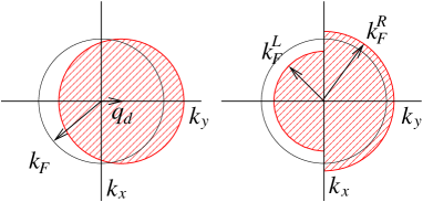
Figure 5: The shifted Fermi sphere (left) and the two-Fermi radii (right) occupations in 2DEG. The occupied states are shown as filled areas, have both identical current density and electronic density but differ in higher moments of $k$.

We have stated that the result for the spin-polarization, Eq. 14, is independent of the considered non-equilibrium occupations of electronic states to the first order in the the spin-orbit coupling $\alpha_{E}$. This is true as long as the current density in the system is the same for all of these considered occupations. Let us consider two simple models of occupations: (1) the “two-Fermi radii model” (2FR), frequently used within the coherent transport with the occupancies dictated by the left and right macroscopic electrodes with Fermi momenta $k_{F}^{R}$ and $k_{F}^{L}$ respectively Mera05 attached to the sample at its ends (Fig. 5, right), and (2) the shifted Fermi distribution function (ShF), used within the main text (Fig. 5, left) From this one immediately sees that the contribution to the spin polarization that is linear in $\alpha_{E}$ in Eq. 11, and therefore also linear in the momentum $k_{y}(=q)$, will be independent of the particular form of the occupations as long as the zero-th and the first moments are identical.

Apart from this, the 2FR and ShF occupations represent two different situations: the former is suited for very short ballistic systems and it directly facilitates interpretation of the results in terms of the difference in electro-chemical potentials of the electrodes, $\Delta\mu=(1/2)\left((k_{F}^{L})^{2}-(k_{F}^{R})^{2}\right)$. The latter is related to the current density inside the sample through

$$j = \int\frac{dk_{x}dk_{y}}{4\pi^{2}}n(k_{x},k_{y})k_{y}=\frac{1}{3\pi^{2}}\left((k_{F}^{R})^{3}-(k_{F}^{L})^{3}\right)$$ (24)

$$\approx \frac{1}{\pi^{2}}\sqrt{2E_{F}}\Delta\mu,$$ (25)

where the occupation factor, $n(k_{x},k_{y})=2$ (spin degeneracy in the unperturbed system) for the occupied states shown in Fig. 5 and $n(k_{x},k_{y})=0$ otherwise. Eq. 25 gives the linear expansion in the applied bias $\Delta\mu$. No such simple connection to the applied bias voltage can be made for the ShF occupation. On the other hand, ShF is suitable for longer samples, where electrons’ scattering leads to partial equilibration of the distribution function Rech09 . This is then characterized with the drift momentum, $q_{d}$, which gives the current density

$$j=n_{2D}q_{d}=\frac{E_{F}}{\pi}q_{d}.$$ (26)

Since the samples we consider are typically longer than the electron’s coherence length, we have used the ShF occupations within the main text. For completeness we give also the results for the 2FR case. The spin polarization per unit length of the sample to third order in $\alpha_{E}$ is

$$m_{z}=-\frac{\alpha_{E}}{\pi^{2}}\sqrt{2E_{F}}\Delta\mu-\frac{2\alpha_{E}^{3}\Delta V}{3\pi^{2}}E_{F}^{3/2}\Delta\mu-\frac{4\alpha_{E}^{3}}{45\pi^{2}}E_{F}^{5/2}\Delta\mu$$ (27)

which after expressing the applied bias in terms of the current density results in

$$m_{z}=-\alpha_{E}j-\frac{2\alpha_{E}^{3}\Delta V}{3}E_{F}j+\frac{4\alpha_{E}^{3}}{45}E_{F}^{2}j.$$ (28)

Comparing the last equation with Eq. 14 we see that while the first order term is identical for both occupations, the higher orders differ by a numerical prefactor. Both of these are larger in the case of partially equilibrated shifted Fermi-like occupations.

References

- (1) Y. K. Kato, R. C. Myers, A. C. Gossard, and D. D. Awschalom, Science 306, 1910 (2004).
- (2) V. Sih, R. C. Myers, Y. K. Kato, W. H. Lau, A. C. Gossard, and D. D. Awschalom, Nature Physics 1, 31 (2005).
- (3) J. Wunderlich, B. Kaestner, J. Sinova, and T. Jungwirth, Phys. Rev. Lett. 94, 047204 (2005).
- (4) V. Sih, Y. K. Kato, and D. D. Awschalom, Physics World Nov, 33 (2005).
- (5) J. Sinova, D. Culcer, Q. Niu, N. A. Sinitsyn, T. Jungwirth, and A. H. MacDonald, Phys. Rev. Lett. 92, 126603 (2004).
- (6) J. I. Inoue, G. E. W. Bauer, and L. W. Molenkamp, Phys. Rev. B 70, 041303(R) (2004).
- (7) E. I. Rashba, Phys. Rev. B 70, 201309(R) (2004).
- (8) B. K. Nikolic, S. Souma, L. P. Zârbo, and J. Sinova, Phys. Rev. Lett. 95, 046601 (2005).
- (9) C. P. Moca and D. C. Marinescu, Phys. Rev. B 75, 035325 (2006).
- (10) V. A. Zyuzin, P. G. Silvestrov, and E. G. Mishchenko, Phys. Rev. Lett. 99, 106601 (2007).
- (11) A. Reynoso, G. Usaj, and C. A. Balseiro, Phys. Rev. B 73, 115342 (2006).
- (12) V. Teodorescu and R. Winkler, Phys. Rev. B 80, 041311(R) (2009).
- (13) E. B. Sonin, arXiv:0909.3156v1 [cond-mat.mes-hall] (2009).
- (14) G. Usaj and C. A. Balseiro, EPL (Europhysics Letters) 72, 631 (2005).
- (15) J. Yao and Z. Q. Yang, Phys. Rev. B 73, 033314 (2006).
- (16) Z. Li and Z. Yang, Phys. Rev. B 77, 205322 (2008).
- (17) K. Hattori and H. Okamoto, Phys. Rev. B 74, 155321 (2006).
- (18) Y. Xing, Q. F. Sun, L. Tang, and J. P. Hu, Phys. Rev. B 74, 155313 (2006).
- (19) S. Bellucci and P. Onorato, Phys. Rev. B 73, 045329 (2006).
- (20) S. Bellucci and P. Onorato, Phys. Rev. B 75, 235326 (2007).
- (21) Y. Jiang and L. Hu, Phys. Rev. B 74, 075302 (2006).
- (22) P. Bokes, F. Corsetti, and R. W. Godby, Phys. Rev. Lett. 101, 046402 (2008).
- (23) P. Debray, J. Wan, S. M. S. Rahman, R. S. Newrock, M. Cahay, A. T. Ngo, S. E. Ulloa, S. T. Herbert, M. Muhammad, and M. Johnson, arXiv:0901.2185v1 [cond-mat.mes-hall] (2009).
- (24) J. J. Krich and B. I. Halperin, Physical Review B (Condensed Matter and Materials Physics) 78, 035338 (2008).
- (25) T. Yokoyama and M. Eto, Physical Review B (Condensed Matter and Materials Physics) 80, 125311 (2009).
- (26) H. A. Engel, E. I. Rashba, and B. I. Halperin, Phys. Rev. Lett. 95, 166605 (2005).
- (27) R. Winkler, Spin-Orbit Coupling Effects in Two-Dimensional Electron and Hole System (Springer, New York, 2003).
- (28) P. Bokes and R. W. Godby, Phys. Rev. B 68, 125414 (2003).
- (29) P. Bokes, H. Mera, and R. W. Godby, Phys. Rev. B 72, 165425 (2005).
- (30) J. Rech, T. Micklitz, and K. A. Matveev, Phys. Rev. Lett. 102, 116402 (2009).
- (31) A. Liebsch, Electornic excitations at metal surfaces (Plenum Press, New York, 1997).
- (32) H. Mera, P. Bokes, and R. W. Godby, Phys. Rev. B 72, 085311 (2005).