Almost local metrics on shape space of hypersurfaces in $n$-space

Abstract.

This paper extends parts of the results from [P.W.Michor and D. Mumford, Appl. Comput. Harmon. Anal., 23 (2007), pp. 74–113] for plane curves to the case of hypersurfaces in $\mathbb{R}^{n}$. Let $M$ be a compact connected oriented $n-1$ dimensional manifold without boundary like the sphere or the torus. Then shape space is either the manifold of submanifolds of $\mathbb{R}^{n}$ of type $M$, or the orbifold of immersions from $M$ to $\mathbb{R}^{n}$ modulo the group of diffeomorphisms of $M$. We investigate almost local Riemannian metrics on shape space. These are induced by metrics of the following form on the space of immersions:

$$G_{f}(h,k)=\int_{M}\Phi(\operatorname{Vol}(f),\operatorname{Tr}(L))\bar{g}(h,k)\operatorname{vol}(f^{*}\bar{g}),$$

where $\bar{g}$ is the Euclidean metric on $\mathbb{R}^{n}$, $f^{*}\bar{g}$ is the induced metric on $M$, $h,k\in C^{\infty}(M,\mathbb{R}^{n})$ are tangent vectors at $f$ to the space of embeddings or immersions, where $\Phi:\mathbb{R}^{2}\to\mathbb{R}_{>0}$ is a suitable smooth function, $\operatorname{Vol}(f)=\int_{M}\operatorname{vol}(f^{*}\bar{g})$ is the total hypersurface volume of $f(M)$, and the trace $\operatorname{Tr}(L)$ of the Weingarten mapping is the mean curvature. For these metrics we compute the geodesic equations both on the space of immersions and on shape space, the conserved momenta arising from the obvious symmetries, and the sectional curvature. For special choices of $\Phi$ we give complete formulas for the sectional curvature. Numerical experiments illustrate the behavior of these metrics.

SIAM J. Imaging Sci. 5 (2012), pp. 244-310.

Contents

91 Introduction
92 Shape space and the Hamiltonian approach
93 Differential geometry of surfaces and notation
94 Variational formulas
95 The geodesic equation on $\operatorname{Imm}(M,\mathbb{R}^{n})$
96 The geodesic equation on $B_{i}(M,\mathbb{R}^{n})$
97 Sectional curvature on $B_{i}(M,\mathbb{R}^{n})$
98 Geodesic distance on $B_{i}(M,\mathbb{R}^{n})$
99 The set of concentric spheres
10 Special cases of almost local metrics
11 Numerical results
90 References
90 The AMPL model file

1. INTRODUCTION

Many procedures in science, engineering, and medicine produce data in the form of shapes of point clouds in $\mathbb{R}^{n}$. If one expects such a cloud to follow roughly a submanifold of a certain type in $\mathbb{R}^{n}$, then it is of utmost importance to describe the space of all possible submanifolds of this type (we call it a shape space hereafter) and equip it with a significant metric which is able to distinguish special features of the shapes. Almost local metrics are a contribution towards this aim.

This paper benefited from discussions with David Mumford, Hermann Schichl, who taught us about the use of AMPL, Johannes Wallner and Tilak Ratnanather. Parts of this paper can be found in the Ph.D. thesis of Martin Bauer [3].

1.1. Reading suggestions

A reader who wants to see results before immersing himself in the theoretical background is recommended to pick up the necessary definitions in the introduction and to jump directly to the last two sections containing special cases and numerical results. In section 2 we build the fundaments for shape analysis in a Riemannian setting. Section 3 presents background material in differential geometry and can serve as a reference for our notation. Throughout this work we will use covariant derivatives of vector fields along immersions. This concept might not be known to all readers; thus we have decided to give a careful description in section 3.5. The main results of the work are in sections 6–11.

In the following introduction we give a non-technical presentation of our approach. Parts of it can also be found in the Ph.D. thesis of Philipp Harms [8].

1.2. The Riemannian setting

Most of the metrics used today in data analysis and computer vision are of an ad-hoc and naive nature. One embeds shape space in some Hilbert space or Banach space and uses the distance therein. Shortest paths are then line segments, but they leave shape space quickly. For several reasons the Riemannian setting for shape analysis is a better solution.

• It formalizes an intuitive notion of similarity of shapes: Shapes that differ only by a small deformation are similar to each other. To compare shapes, we measure the length of a deformation. A deformation of a shape is a path in shape space. Remember that in a Riemannian manifold, the geodesic distance between two points is the infimum over the length of all paths connecting them.

• Riemannian metrics on shape space have been used successfully in computer vision for a long time, often without any mention of the underlying metric. Gradient flows for shape smoothing are an example. An underlying metric is needed for the definition of a gradient. Often, the metric used implicitly is the $L^{2}$-metric which has, however, turned out to be too weak.

• The exponential map (if it exists) that is induced by a Riemannian metric permits us to linearize shape space: When shapes are represented as initial velocities of geodesics connecting them to a fixed reference shape, one effectively works in the linear tangent space over the reference shape. Curvature will play an essential role in quantifying the deviation of curved shape space from its linearized approximation.

• The linearization of shape space by the exponential map allows us to do statistics on shape space.

However a disadvantage of the Riemannian approach is that shapes can be compared with each other only when there is a deformation between them, i.e., when they have the same topology.

1.3. Shape spaces

In mathematics and computer vision, shapes have been represented in many ways. Point clouds, meshes, level-sets, graphs of a function, currents, and measures are but some of the possibilities. The notion of shapes underlying this work is that of immersed or embedded submanifolds of $\mathbb{R}^{n}$ of co-dimension one. Any such submanifold can be represented as a fixed immersion or embedding modulo reparametrizations.

The space of all immersions is illustrated in figure 1. The colors are there to help the reader visualize parametrizations. Immersions differing only by a reparametrization are drawn along vertical lines. These lines are the orbits of the reparametrization group. Immersions in the same orbit correspond to the same shape in shape space. In other words, shape space is the space of orbits of the reparametrization group acting on the space of immersions.

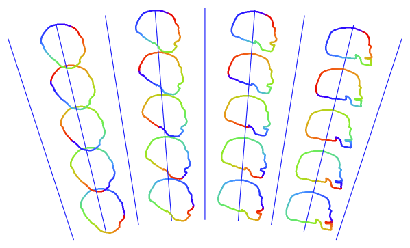
Figure 1. Illustration of the space of immersions of $S^{1}$ in $\mathbb{R}^{2}$.

As mentioned in the previous section, only shapes with the same topology can be compared. Thus we assume that all shapes (i.e., submanifolds) are diffeomorphic to the same compact connected oriented $n-1$ dimensional manifold $M$. We will deal only with smooth shapes. They form the core of actual shape space, which can be viewed as the Cauchy completion with respect to geodesic distance for one of the Riemannian metrics that we treat in this paper. See section 2 for a formal definition of shape space.

1.4. Riemannian metrics on shape space

Riemannian metrics measure infinitesimal deformations. Riemannian metrics on shape space come in two flavors:

• Outer metrics measure how much ambient space has to be deformed in order to yield the desired deformation of the shape. An infinitesimal deformation of ambient space is a vector field on ambient space and could be pictured as a small arrow attached to every point in ambient space; see figure 2.

• Inner metrics measure deformations of the shape itself within a fixed ambient space. An infinitesimal deformation of the shape itself is a vector field along the shape. It could be pictured as a small arrow attached to every point of the shape; see figure 2.

The metrics treated in this work are inner metrics.

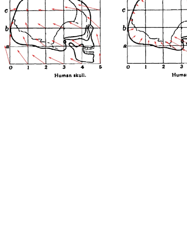
Figure 2. Infinitesimal transformation of ambient space (left) as measured by an outer metric and infinitesimal transformation of the shape itself (right) as measured by an inner metric.

1.5. Where this paper comes from

In [15], Michor and Mumford investigated inner metrics on the shape space of planar curves. The simplest such metric is the $L^{2}$-metric given by

$$G^{0}_{f}(h,k) =\int_{S^{1}}\bar{g}\big{(}h(\theta),k(\theta)\big{)}\,|f^{\prime}(\theta)|\,d\theta,$$

where $f,h,k:S^{1}\to\mathbb{R}^{2}$ are smooth functions. $f$ is the curve representing the shape, and $h,k$ are deformation vector fields of $f$. The Euclidean metric on $\mathbb{R}^{2}$ is denoted by $\bar{g}$. We use integration by arc length $ds=|f^{\prime}(\theta)|\,d\theta$. This makes the metric invariant under reparametrizations of $f,h,k$. This invariance is needed when factoring out reparametrizations; see section 2. Since the metric has to be positive definite, it is natural to require that $f^{\prime}(\theta)\neq 0$ everywhere, i.e., $f$ is an immersion.

Unfortunately it turned out that the $L^{2}$ metric induces vanishing geodesic distance on shape space [15]. This means that any two shapes can be connected by an arbitrarily short path in shape space, when path length is measured with the $L^{2}$ metric. Later in [14] it was found that the vanishing geodesic distance phenomenon for the $L^{2}$-metric occurs also in the more general shape space where $S^{1}$ is replaced by a compact manifold $M$ and Euclidean $\mathbb{R}^{2}$ is replaced by a Riemannian manifold $N$. It also occurs on the full diffeomorphism group $\operatorname{Diff}(N)$. These results together imply vanishing geodesic distance on spaces of immersions.

The discovery of the degeneracy of the $L^{2}$ metric was the starting point of a quest for better Riemannian metrics. A possibility excluding the degenerate paths encountered in [15] is to penalize high length and/or curvature. This led to the investigation of a class of metrics which were called almost local metrics; see [16, 15]. A better name might be weighted $L^{2}$-metrics. They are of the form

$$G^{\Phi}_{f}(h,k)=\int_{S^{1}}\Phi(\ell(f),\kappa_{f}(\theta))\bar{g}\big{(}h(\theta),k(\theta)\big{)}|f^{\prime}(\theta)|\,d\theta,$$

where $\Phi:\mathbb{R}^{2}\to\mathbb{R}_{>0}$ is a suitable smooth function, $\ell(f)=\int_{S^{1}}|f^{\prime}(\theta)|\,d\theta$ is the length of $f$, and $\kappa_{f}$ is the curvature of $f$. If $\Phi=\Phi(\ell(f))$, then this is just a conformal change of the metric; it was proposed and investigated independently in [18] and in [23, 24, 25]. For $\Phi=1+A\kappa_{f}^{2}$, where $A$ is a positive constant, the metric was investigated in great detail in [15].

1.6. Almost local metrics, geodesics, and curvature

In this paper we take up the investigation of almost local metrics from [16] and we generalize it to higher dimensions. For surfaces in $\mathbb{R}^{3}$ this leads to metrics of the form

$$G^{\Phi}_{f}(h,k)=\int_{M}\Phi(\operatorname{Area}(f),\mu)\,\bar{g}(h,k)\,d\operatorname{Area}.$$

Here $M$ is a compact connected oriented two-dimensional manifold, $\bar{g}$ is the Euclidean metric on $\mathbb{R}^{3}$, $f:M\to\mathbb{R}^{3}$ is an immersion, $h,k:M\to\mathbb{R}^{3}$ are seen as deformation vector fields of the immersion, and $\Phi:\mathbb{R}^{3}\to\mathbb{R}_{>0}$ is again a suitable positive smooth function depending on the area of the immersed surface $f(M)$ and on the mean curvature $\mu$. In two dimensions, the mean curvature $\mu=\operatorname{Tr}(L)$ and Gauß curvature $\kappa=\det(L)$ are all the invariants of the Weingarten mapping $L$. However, in this paper we do not treat the metric which involves the Gauß curvature. This is done in the paper [1].

We do not restrict ourselves to surfaces in $\mathbb{R}^{3}$. Instead we treat almost local metrics on spaces of hyper-surfaces in $\mathbb{R}^{n}$. More specifically, these are metrics of the form

$$G^{\Phi}_{f}(h,k)=\int_{M}\Phi(\operatorname{Vol}(f),\operatorname{Tr}(L))\,\bar{g}(h,k)\operatorname{vol}(g).$$

Here $M$ is a compact connected oriented $n-1$ dimensional manifold, $f:M\to\mathbb{R}^{n}$ is an immersion, $h,k:M\to\mathbb{R}^{n}$ are deformation vector fields, and $\Phi:\mathbb{R}^{2}\to\mathbb{R}_{>0}$ is again a suitable positive smooth function. We denote the pullback of the Euclidean metric $\bar{g}$ to $M$ via the immersion $f$ by $g=f^{*}\bar{g}$. It is sometimes called the first fundamental form of the surface and is given in coordinates by $g_{ij}=\bar{g}(\partial_{i}f,\partial_{j}f)$. The natural replacement of $dA$ is the $n-1$ dimensional volume density $\operatorname{vol}(g)$ induced by $g$. In coordinates $u^{1},\ldots u^{n-1}$ on $M$ it is given by $\sqrt{\det(g_{ij})}\,|du^{1}\wedge\cdots\wedge du^{n-1}|$. The total $n-1$ dimensional volume of $f(M)$ is denoted by $\operatorname{Vol}(f)=\int_{M}\operatorname{vol}(g)$. Finally, $\operatorname{Tr}(L)$ is the mean curvature, which is the trace of the Weingarten mapping $L$. See section 3 for a rigorous definition of the objects that are used in the definition of the metric.

As mentioned above, metrics of this form will be called almost local as in [16]. A better name might be weighted $H^{0}$-metrics or weighted $L^{2}$-metrics. It is natural to consider Gauß-curvature weighted metrics as well. This is done in [1]. It might also be worth considering other curvature invariants.

In the theoretical part of this work $\Phi$ is general. The special choices of $\Phi$ investigated in the more practical two last sections are

$$\Phi=\operatorname{Vol}^{k},\quad\Phi=e^{\operatorname{Vol}},\quad\Phi=1+A\operatorname{Tr}(L)^{2k},\quad\Phi=\operatorname{Vol}^{\frac{1+n}{1-n}}+A\frac{\operatorname{Tr}(L)^{2}}{\operatorname{Vol}},$$

where $A>0$ and $k\in\mathbb{N}$ are constants. The last choice of $\Phi$ induces a scale-invariant metric.

The $G^{\Phi}$-metrics are weak Riemannian metrics on the manifold of all immersions $M\to\mathbb{R}^{n}$, which is an open subset of the Fréchet space of all smooth mappings. But we are interested in the induced Riemannian metric on shape space, which is the quotient space under the identification of immersions differing only by a reparametrization; see 2.8. Shape space is difficult to handle, but geodesics on shape space are images of so-called horizontal geodesics on the space of immersions. A geodesic on the manifold of immersions is called horizontal if its velocity vector is a horizontal tangent vector at each time. A tangent vector is called horizontal if it is $G^{\Phi}$-perpendicular to the reparametrization orbits. The length of a horizontal (minimizing) geodesic defines the distance between its endpoints, which is what we are interested in.

In general, geodesics are critical points of the energy functional

$$E(f)=\frac{1}{2}\int_{0}^{1}G^{\Phi}_{f(t)}(\partial_{t}f,\partial_{t}f)\,dt,$$

where $f$ is a smooth curve of immersions. A curve $f(t)$ is a critical point of the horizontal energy functional

$$E^{\text{hor}}(f)=\frac{1}{2}\int_{0}^{1}G^{\Phi}_{f(t)}\big{(}(\partial_{t}f)^{\operatorname{hor}},(\partial_{t}f)^{\operatorname{hor}}\big{)}\,dt$$

if and only if a suitable reparametrization of it is a horizontal geodesic. In the above formula $(\partial_{t}f)^{\operatorname{hor}}$ denotes the horizontal part of the velocity $\partial_{t}f$; see section 2.8.

Almost local metrics have the great advantage that a tangent vector $h:M\to\mathbb{R}^{n}$ with footpoint an immersion $f:M\to\mathbb{R}^{n}$ is horizontal if and only if $h(x)$ is normal to $T_{f(x)}f(M)$ in $\mathbb{R}^{n}$ for all $x\in M$; see section 6.1. Therefore the horizontal energy for almost local metrics is given by an easy and computable formula. This makes the numerical approach in this paper possible; see section 11. But an analytical proof of the existence of critical points for the horizontal energy (which can be viewed as an anisotropic plateau problem) is still lacking. The simple form of the horizontal bundle also opens the way to computations of sectional curvature on shape space; see section 7. We are interested in sectional curvature because it will eventually be important for doing statistics on shape space and for the computation of conjugate points. Furthermore, unbounded positive sectional curvature might be related to vanishing geodesic distance (see [14]).

1.7. Contributions of this work

Almost local metrics are generalized to higher dimensions. Some estimates for geodesic distance on shape space are proven. They show that almost local metrics with suitable functions $\Phi$ overcome the degeneracy of the $L^{2}$ metric. In addition, almost local metrics are compared to the Fréchet metric.

The geodesic equation and conserved quantities are calculated on shape space and on the full space of immersions. For this aim the Hamiltonian formalism developed in [16] is updated to the more general situation here. Furthermore, the Riemann curvature tensor is calculated on shape space. It contains some negative, positive, and indefinite terms. Explicit formulas for special choices of $\Phi$ are given.

For all these calculations, first and second derivatives of the metric, volume form, second fundamental form and other curvature terms are developed. The derivatives are taken with respect to the immersion inducing these objects.

The last section contains numerical experiments for geodesics. We do only boundary value problems and no initial value problems (it is not clear if the initial value problem is well posed). We use Mathematica to set up the triangulation of the surfaces, feed this into AMPL (a modeling software developed for optimization), and use the solver IPOPT. The numerical results are tested on the totally geodesic subspace of concentric spheres where we also have analytic solutions. Then we study translations and deformations of surfaces for various metrics and discuss the appearing phenomena.

For the sake of simplicity we have restricted ourselves to the shape space of hyper-surfaces in $\mathbb{R}^{n}$. The more general case of arbitrary co-dimension and $\mathbb{R}^{n}$ replaced by a non-flat Riemannian manifold $(N,\bar{g})$ will be treated in another paper.

2. Shape space and the Hamiltonian approach

The aim of this chapter is to develop a rigorous notion of shape space, to derive the geodesic equation on shape space, and to calculate the conserved momenta.

2.1. Manifolds of immersions and embeddings and the diffeomorphism group

Mathematically, parametrized surfaces will be modeled as immersions or embeddings of one manifold into another. We call immersions and embeddings parametrized since a change in their parametrization (i.e., applying a diffeomorphism on the domain of the function) results in a different object. We will deal with the following sets of functions:

(1) $$\operatorname{Emb}(M,\mathbb{R}^{n})\subset\operatorname{Imm}(M,\mathbb{R}^{n})\subset C^{\infty}(M,\mathbb{R}^{n}).$$

$C^{\infty}(M,\mathbb{R}^{n})$ is the set of smooth functions from $M$ to $\mathbb{R}^{n}$. $\operatorname{Imm}(M,\mathbb{R}^{n})$ is the set of all immersions of $M$ into $\mathbb{R}^{n}$, i.e., all functions $f\in C^{\infty}(M,\mathbb{R}^{n})$ such that $T_{x}f$ is injective for all $x\in M$. $\operatorname{Emb}(M,\mathbb{R}^{n})$ is the set of all embeddings of $M$ into $\mathbb{R}^{n}$, i.e., all immersions $f$ that are a homeomorphism onto their image. In most cases, immersions will be used since this is the most general setting. Working with embeddings instead of immersions makes a difference in section 8.

Since $M$ is compact, by assumption it follows that $C^{\infty}(M,\mathbb{R}^{n})$ is a Fréchet manifold [11, section 42.3]. All inclusions in (1) are inclusions of open subsets. Therefore, all function spaces in (1) are Fréchet manifolds as well.

The tangent bundle of the manifold of immersions is

$$T\operatorname{Imm}(M,\mathbb{R}^{n})=\operatorname{Imm}(M,\mathbb{R}^{n})\times C^{\infty}(M,\mathbb{R}^{n})\subset C^{\infty}(M,\mathbb{R}^{n}\times\mathbb{R}^{n}),$$

and the cotangent bundle is $T^{*}\operatorname{Imm}(M,\mathbb{R}^{n})=\operatorname{Imm}(M,\mathbb{R}^{n})\times\mathcal{D}^{\prime}(M)^{n}$, where the second factor consists of $n$-tuples of distributions in $\mathcal{D}^{\prime}(M)=C^{\infty}(M)^{\prime}$, which is the space of distributional sections of the density bundle.

By $\operatorname{Diff}(M)$ we will denote the group of all smooth diffeomorphisms. $\operatorname{Diff}(M)$ is a Fréchet manifold as well, since it is an open subset of $C^{\infty}(M,M)$. It is an infinite dimensional Lie group in the sense of [11, section 43]. The diffeomorphism group $\operatorname{Diff}(M)$ acts smoothly on $C^{\infty}(M,\mathbb{R}^{n})$ and its subspaces $\operatorname{Imm}(M,\mathbb{R}^{n})$ and $\operatorname{Emb}(M,\mathbb{R}^{n})$ by composition from the right. The action is given by the mapping

$$\operatorname{Imm}(M,\mathbb{R}^{n})\times\operatorname{Diff}(M)\to\operatorname{Imm}(M,\mathbb{R}^{n}),\qquad(f,\varphi)\mapsto r(f,\varphi)=r^{\varphi}(f)=f\circ\varphi.$$

The tangent prolongation of this group action is given by the mapping

$$T(r^{\varphi}):T\operatorname{Imm}(M,\mathbb{R}^{n})\times\operatorname{Diff}(M) \to T\operatorname{Imm}(M,\mathbb{R}^{n}),$$

$$(f,h,\varphi) \mapsto(f\circ\varphi,h\circ\varphi).$$

We will sometimes use the abbreviations $\operatorname{Emb},\operatorname{Imm}$, and $\operatorname{Diff}$ when the domain and co-domain of the functions are clear from the context.

2.2. Riemannian metrics on the manifold of immersions

In this work we consider smooth Riemannian metrics on $\operatorname{Imm}(M,\mathbb{R}^{n})$, i.e., smooth mappings

$$G:\operatorname{Imm}(M,\mathbb{R}^{n})\times C^{\infty}(M,\mathbb{R}^{n})\times C^{\infty}(M,\mathbb{R}^{n})\to\mathbb{R},$$

$$(f,h,k)\mapsto G_{f}(h,k),\quad\text{ bilinear in }h,k,$$

$$G_{f}(h,h)>0\quad\text{ for }h\neq 0.$$

Each such metric is weak in the sense that $G_{f}$, viewed as bounded linear mapping

$$G_{f}:T_{f}\operatorname{Imm}(M,\mathbb{R}^{n})=C^{\infty}(M,\mathbb{R}^{n}) \to T_{f}^{*}\operatorname{Imm}(M,\mathbb{R}^{n})=\mathcal{D}^{\prime}(M)^{n},$$

$$G:T\operatorname{Imm}(M,\mathbb{R}^{n}) \to T^{*}\operatorname{Imm}(M,\mathbb{R}^{n}),$$

$$G(f,h) =(f,G_{f}(h,\;.\;)),$$

is injective but can never be surjective. We shall need also its tangent mapping

$$TG:T(T\operatorname{Imm}(M,\mathbb{R}^{n})) \to T(T^{*}\operatorname{Imm}(M,\mathbb{R}^{n})).$$

We write a tangent vector to $T\operatorname{Imm}(M,\mathbb{R}^{n})$ as $(f,h;k,v)$, where $(f,h)\in T\operatorname{Imm}(M,\mathbb{R}^{n})$ is its footpoint, $k$ is its vector component in the $\operatorname{Imm}(M,\mathbb{R}^{n})$-direction, and where $v$ is its component in the $C^{\infty}(M,\mathbb{R}^{n})$-direction.

Then $TG$ is given by

$$TG(f,h;k,v)=(f,G_{f}(h,\;.\;);k,D_{(f,k)}G_{f}(h,\;.\;)+G_{f}(v,\;.\;)).$$

Note that only these smooth functions on $\operatorname{Imm}(M,\mathbb{R}^{n})$ whose derivatives lie in the image of $G$ in the cotangent bundle have $G$-gradients. This requirement has only to be satisfied for the first derivative; for the higher ones it follows (see [11]). We shall denote by $C^{\infty}_{G}(\operatorname{Imm}(M,\mathbb{R}^{n}))$ the space of such smooth functions.

In what follows we shall further assume that that the weak Riemannian metric $G$ itself admits $G$-gradients with respect to the variable $f$ in the following sense:

$$\boxed{D_{(f,m)}G_{f}(h,k)=G_{f}(m,H_{f}(h,k))=G_{f}(K_{f}(m,h),k),}\quad\text{ where }$$

$$H,K:\operatorname{Imm}(M,\mathbb{R}^{n})\times C^{\infty}(M,\mathbb{R}^{n})\times C^{\infty}(M,\mathbb{R}^{n})\to C^{\infty}(M,\mathbb{R}^{n})$$

$$\hskip 180.67499pt(f,h,k)\mapsto H_{f}(h,k),K_{f}(h,k)$$

$$\text{are smooth and bilinear in }h,k.$$

Note that $H$ and $K$ could be expressed in abstract index notation as $g_{ij,k}g^{kl}$ and $g_{ij,k}g^{il}$. We will check and compute these gradients for several concrete metrics below.

2.3. The fundamental symplectic form on $T\operatorname{Imm}(M,\mathbb{R}^{n})$ induced by a weak Riemannian metric

The basis of Hamiltonian theory is the natural 1-form on the cotangent bundle $T^{*}\operatorname{Imm}(M,\mathbb{R}^{n})$ given by

$$\Theta:T(T^{*}\operatorname{Imm}(M,\mathbb{R}^{n}))=\operatorname{Imm}(M,\mathbb{R}^{n})\times\mathcal{D}^{\prime}(M)^{n}\times C^{\infty}(M,\mathbb{R}^{n})\times\mathcal{D}^{\prime}(M)^{n}\to\mathbb{R},$$

$$(f,\alpha;h,\beta)\mapsto\langle\alpha,h\rangle.$$

The pullback via the mapping $G:T\operatorname{Imm}(M,\mathbb{R}^{n})\to T^{*}\operatorname{Imm}(M,\mathbb{R}^{n})$ of $\Theta$ is

$$(G^{*}\Theta)_{(f,h)}(f,h;k,v)=G_{f}(h,k).$$

Thus the symplectic form $\omega=-dG^{*}\Theta$ on $T\operatorname{Imm}(M,\mathbb{R}^{n})$ can be computed as follows, where we use the constant vector fields $(f,h)\mapsto(f,h;k,v)$:

$$\omega_{(f,h)} ((k_{1},v_{1}),(k_{2},v_{2}))=-d(G^{*}\Theta)((k_{1},v_{1}),(k_{2},v_{2}))|_{(f,h)}$$

$$=-D_{(f,k_{1})}G_{f}(h,k_{2})-G_{f}(v_{1},k_{2})+D_{(f,k_{2})}G_{f}(h,k_{1})+G_{f}(v_{2},k_{1})$$

(1) $$=G_{f}\big{(}k_{2},H_{f}(h,k_{1})-K_{f}(k_{1},h)\big{)}+G_{f}(v_{2},k_{1})-G_{f}(v_{1},k_{2}).$$

2.4. The Hamiltonian vector field mapping

Here we compute the Hamiltonian vector field $\operatorname{grad}^{\omega}(F)$ associated to a smooth function $F$ on the tangent space $T\operatorname{Imm}(M,\mathbb{R}^{n})$; that is $F\in C^{\infty}_{G}(\operatorname{Imm}(M,\mathbb{R}^{n})\times C^{\infty}(M,\mathbb{R}^{n}))$ assuming that it has smooth $G$-gradients in both factors. See [11, section 48]. Using the explicit formulas in section 2.3, we have

$$\omega_{(f,h)}\left(\operatorname{grad}^{\omega}(F)(f,h),(k,v)\right)$$

$$\quad=\omega_{(f,h)}\left((\operatorname{grad}_{1}^{\omega}(F)(f,h),\operatorname{grad}_{2}^{\omega}(F)(f,h)),(k,v)\right)$$

$$\quad=G_{f}\big{(}k,H_{f}\big{(}h,\operatorname{grad}_{1}^{\omega}(F)(f,h)\big{)}\big{)}-G_{f}(K_{f}(\operatorname{grad}_{1}^{\omega}(F)(f,h),h),k)$$

$$\qquad+G_{f}(v,\operatorname{grad}_{1}^{\omega}(F)(f,h))-G_{f}(\operatorname{grad}_{2}^{\omega}(F)(f,h),k).$$

On the other hand, by the definition of the $\omega$-gradient we have

$$\omega_{(f,h)}\left(\operatorname{grad}^{\omega}(F)(f,h),(k,v)\right)=dF(f,h)(k,v)=D_{(f,k)}F(f,h)+D_{(h,v)}F(f,h)$$

$$=G_{f}(\operatorname{grad}_{1}^{G}(F)(f,h),k)+G_{f}(\operatorname{grad}_{2}^{G}(F)(f,h),v),$$

and we get the expression of the Hamiltonian vector field:

$$\boxed{\begin{aligned} \operatorname{grad}_{1}^{\omega}(F)(f,h)&=\operatorname{grad}_{2}^{G}(F)(f,h),\\ \operatorname{grad}_{2}^{\omega}(F)(f,h)&=\!-\!\operatorname{grad}_{1}^{G}(F)(f,h)\\ &\quad+H_{f}\big{(}h,\operatorname{grad}_{2}^{G}(F)(f,h)\big{)}-K_{f}(\operatorname{grad}_{2}^{G}(F)(f,h),h).\end{aligned}}$$

Note that for a smooth function $F$ on $T\operatorname{Imm}(M,\mathbb{R}^{n})$ the $\omega$-gradient exists if and only if both $G$-gradients exist.

2.5. The geodesic equation on the manifold of immersions

The geodesic flow is defined by a vector field on $T\operatorname{Imm}(M,\mathbb{R}^{n})$. One way to define this vector field is as the Hamiltonian vector field of the energy function

$$E(f,h)=\frac{1}{2}G_{f}(h,h),\qquad E:\operatorname{Imm}(M,\mathbb{R}^{n})\times C^{\infty}(M,\mathbb{R}^{n})\to\mathbb{R}.$$

The two partial $G$-gradients are

$$G_{f}(\operatorname{grad}_{2}^{G}(E)(f,h),v) =d_{2}E(f,h)(v)=G_{f}(h,v),$$

$$\operatorname{grad}_{2}^{G}(E)(f,h) =h,$$

$$G_{f}(\operatorname{grad}_{1}^{G}(E)(f,h),k) =d_{1}E(f,h)(k)=\tfrac{1}{2}D_{(f,k)}G_{f}(h,h)$$

$$=\tfrac{1}{2}G_{f}(k,H_{f}(h,h)),$$

$$\operatorname{grad}_{1}^{G}(E)(f,h) =\tfrac{1}{2}H_{f}(h,h).$$

Thus the geodesic vector field is

$$\operatorname{grad}_{1}^{\omega}(E)(f,h) =h$$

$$\operatorname{grad}_{2}^{\omega}(E)(f,h) =\tfrac{1}{2}H_{f}(h,h)-K_{f}(h,h)$$

and the geodesic equation becomes

$$\begin{cases}f_{t}&=h,\\ h_{t}&=\tfrac{1}{2}H_{f}(h,h)-K_{f}(h,h),\end{cases}\quad\text{ or }\quad\boxed{f_{tt}=\tfrac{1}{2}H_{f}(f_{t},f_{t})-K_{f}(f_{t},f_{t}).}$$

This is nothing but the usual formula for the geodesic flow using the Christoffel symbols expanded out using the first derivatives of the metric tensor.

2.6. The momentum mapping for a $G$-isometric group action

We consider now a (possibly infinite dimensional regular) Lie group with Lie algebra $\mathfrak{g}$ with a right action $g\mapsto r^{g}$ by isometries on $\operatorname{Imm}(M,\mathbb{R}^{n})$. Denote by $\mathfrak{X}(\operatorname{Imm}(M,\mathbb{R}^{n}))$ the set of vector fields on $\operatorname{Imm}(M,\mathbb{R}^{n})$. Then we can specify this action by the fundamental vector field mapping $\zeta:\mathfrak{g}\to\mathfrak{X}(\operatorname{Imm}(M,\mathbb{R}^{n}))$, which will be a bounded Lie algebra homomorphism. The fundamental vector field $\zeta_{X},X\in\mathfrak{g}$, is the infinitesimal action in the sense that

$$\zeta_{X}(f)=\partial_{t}|_{0}r^{\exp(tX)}(f).$$

We also consider the tangent prolongation of this action on $T\operatorname{Imm}(M,\mathbb{R}^{n})$, where the fundamental vector field is given by

$$\zeta_{X}^{T\operatorname{Imm}}:(f,h)\mapsto(f,h;\zeta_{X}(f),D_{(f,h)}(\zeta_{X})(f)=:\zeta^{\prime}_{X}(f,h)).$$

The basic assumption is that the action is by isometries,

$$G_{f}(h,k)=((r^{g})^{*}G)_{f}(h,k)=G_{r^{g}(f)}(T_{f}(r^{g})h,T_{f}(r^{g})k).$$

Differentiating this equation at $g=e$ in the direction $X\in\mathfrak{g}$, we get

(1) $$0=D_{(f,\zeta_{X}(f))}G_{f}(h,k)+G_{f}(\zeta^{\prime}_{X}(f,h),k)+G_{f}(h,\zeta^{\prime}_{X}(f,k)).$$

The key to the Hamiltonian approach is to define the group action by Hamiltonian flows. We define the momentum map $j:\mathfrak{g}\to C^{\infty}_{G}(T\operatorname{Imm}(M,\mathbb{R}^{n}),\mathbb{R})$ by

$$\boxed{j_{X}(f,h)=G_{f}(\zeta_{X}(f),h).}$$

Equivalently, since this map is linear, it is often written as a map

$$\mathcal{J}:T\operatorname{Imm}(M,\mathbb{R}^{n})\rightarrow\mathfrak{g}^{\prime},\qquad\langle\mathcal{J}(f,h),X\rangle=j_{X}(f,h).$$

The main property of the momentum map is that it fits into the following commutative diagram and is a homomorphism of Lie algebras:

where $\mathfrak{X}(T\operatorname{Imm},\omega)$ is the space of vector fields on $T\operatorname{Imm}$ whose flow leaves $\omega$ fixed. Note also that $\mathcal{J}$ is equivariant for the group action. See [16] for more details.

By Noether’s theorem, along any geodesic $t\mapsto f(t,\;.\;)$ this momentum mapping is constant; thus for any $X\in\mathfrak{g}$ we have

$$\boxed{\quad\langle\mathcal{J}(f,f_{t}),X\rangle=j_{X}(f,f_{t})=G_{f}(\zeta_{X}(f),f_{t})\quad\text{ is constant in }t.\quad}$$

We can apply this construction to the following group actions:

• The smooth right action of the group $\operatorname{Diff}(M)$ on $\operatorname{Imm}(M,\mathbb{R}^{n})$, given by composition from the right: $f\mapsto f\circ\varphi$ for $\varphi\in\operatorname{Diff}(M)$.

  For $X\in\mathfrak{X}(M)$ the fundamental vector field is then given by

  $$\zeta^{\operatorname{Diff}}_{X}(f)=\zeta_{X}(f)=X(f)=\partial_{t}|_{0}(f\circ\operatorname{Fl}^{X}_{t})=df.X,$$

  where $\operatorname{Fl}^{X}_{t}$ denotes the flow of $X$. The reparametrization momentum, for any vector field $X$ on $M$ is thus

  $$j_{X}(f,h)=G_{f}(df.X,h).$$

  Assuming the metric is reparametrization invariant, it follows that on any geodesic $f(x,t)$, the expression $G_{f}(df.X,f_{t})$ is constant for all $X$.

• The left action of the Euclidean motion group $\mathbb{R}^{n}\rtimes SO(n)$ on $\operatorname{Imm}(M,\mathbb{R}^{n})$ given by $f\mapsto Af+B$ for $(B,A)\in\mathbb{R}^{n}\times SO(n)$. The fundamental vector field mapping is

  $$\zeta_{(B,X)}(f) =Xf+B.$$

  The linear-momentum is thus $G_{f}(B,h),B\in\mathbb{R}^{n}$, and if the metric is translation invariant, $G_{f}(B,f_{t})$ will be constant along geodesics for every $B\in\mathbb{R}^{n}$. The angular-momentum is similarly $G_{f}(X.f,h),X\in\mathfrak{s}\mathfrak{o}(n)$, and if the metric is rotation-invariant, then $G_{f}(X.f,f_{t})$ will be constant along geodesics for each $X\in\mathfrak{s}\mathfrak{o}(n)$.

• The action of the scaling group of $\mathbb{R}$ given by $c\mapsto e^{r}f$, with fundamental vector field $\zeta_{a}(f)=a.f$.

  If the metric is scale-invariant, then the scaling momentum $G_{f}(f,f_{t})$ will also be invariant along geodesics.

2.7. Shape space

As discussed in the introduction, by a shape we mean a smoothly immersed or embedded hypersurface in $\mathbb{R}^{n}$ which is diffeomorphic to a fixed compact, connected, and oriented manifold $M$ of dimension $n-1$. The space of these shapes will be denoted $B_{i}(M,\mathbb{R}^{n})$ or $B_{e}(M,\mathbb{R}^{n})$ and viewed as the quotient

$$B_{e}(M,\mathbb{R}^{n})=\operatorname{Emb}(M,\mathbb{R}^{n})/\operatorname{Diff}(M)\text{ or }B_{i}(M,\mathbb{R}^{n})=\operatorname{Imm}(M,\mathbb{R}^{n})/\operatorname{Diff}(M).$$

In [11, section 44.1] it is shown that $B_{e}(M,\mathbb{R}^{n})$ is a manifold again. $B_{i}(M,\mathbb{R}^{n})$ is, however, no longer a manifold but an orbifold with finite isotropy groups; see [5]. We will sometimes use the abbreviations $B_{i}$ and $B_{e}$ when it is clear what the domain and co-domain of the functions are.

More generally, a shape will be an element of the Cauchy completion (i.e., the metric completion for the geodesic distance) of $B_{i}(M,\mathbb{R}^{n})$ with respect to a suitably chosen Riemannian metric. This will allow for corners.

2.8. Riemannian submersions and the metric on shape space

We will always assume that a $\operatorname{Diff}(M)$-invariant Riemannian metric on $\operatorname{Imm}(M,\mathbb{R}^{n})$ is given. Then there is a unique Riemannian metric on the quotient space $B_{i}(M,\mathbb{R}^{n})$ such that the quotient map $\pi:\operatorname{Imm}(M,\mathbb{R}^{n})\rightarrow B_{i}(M,\mathbb{R}^{n})$ is a Riemannian submersion. This is the construction that we use to induce a metric on shape space.

Let $\operatorname{ker}(T\pi)\subset T\operatorname{Imm}(M,\mathbb{R}^{n})$ be the vertical bundle. The horizontal bundle is its orthogonal complement with respect to the metric $G$. Then $T_{\pi(f)}B_{i}(M,\mathbb{R}^{n})$ is isometric to the horizontal bundle at $f\in\operatorname{Imm}(M,\mathbb{R}^{n})$. Note that the horizontal bundle depends on the definition of the metric. For almost local metrics, it consists of vector fields along $f$ that are everywhere normal to $f$; see section 6.1 .

By the conservation of the reparametrization momentum, geodesics in the space of immersions with horizontal initial velocity stay horizontal for all time. Such geodesics project down to geodesics in shape space because $\pi$ is a Riemannian submersion. See [13, section 26] for a proof of this fact. We will show in section 6.1 that almost local metrics have the property that any curve in shape space can be lifted to a horizontal curve of immersions. This implies that instead of solving the geodesic equation on shape space one can equivalently solve the equation for horizontal geodesics in the space of immersions.

3. Differential geometry of surfaces and notation

In this section we will present and develop the differential geometric tools that are needed to deal with immersed surfaces. The most important point is a rigorous treatment of the covariant derivative and related concepts.

In [2, section 2] one can find some parts of this section in a more general setting. We use the notation of [13]. Some of the definitions can also be found in [9].

3.1. Tensor bundles and tensor fields

We will deal with the tensor bundles

Here $T^{r}_{s}M$ denotes the bundle of $\left(\begin{smallmatrix}r\\ s\end{smallmatrix}\right)$-tensors on $M$, i.e.,

$$T^{r}_{s}M=\bigotimes^{r}TM\otimes\bigotimes^{s}T^{*}M,$$

and $f^{*}T\mathbb{R}^{n}$ is the pullback of the bundle $T\mathbb{R}^{n}$ via $f$; see [13, section 17.5]. A tensor field is a section of a tensor bundle. Generally, when $E$ is a bundle, the space of its sections will be denoted by $\Gamma(E)$.

To clarify the notation that will be used later, some examples of tensor bundles and tensor fields are given now.

• $\operatorname{End}(TM)=L(TM,TM)=T^{1}_{1}M$ is the bundle of endomorphisms of $TM$.

• $S^{k}T^{*}M=L^{k}_{\operatorname{sym}}(TM;\mathbb{R})$ is the bundle of symmetric $\left(\begin{smallmatrix}0\\ k\end{smallmatrix}\right)$-tensors.

• $S^{2}_{>0}T^{*}M$ is the bundle of symmetric positive definite $\left(\begin{smallmatrix}0\\ 2\end{smallmatrix}\right)$-tensors.

• $\Lambda^{k}T^{*}M=L^{k}_{\operatorname{alt}}(TM;\mathbb{R})$ is the bundle of alternating $\left(\begin{smallmatrix}0\\ k\end{smallmatrix}\right)$-tensors.

• $\Omega^{r}(M)=\Gamma(\Lambda^{r}T^{*}M)$ is the space of differential forms.

• $\mathfrak{X}(M)=\Gamma(TM)$ is the space of vector fields.

• $\Gamma(f^{*}T\mathbb{R}^{n})\cong\big{\{}h\in C^{\infty}(M,T\mathbb{R}^{n}):\pi_{N}\circ h=f\big{\}}$ is the space of vector fields along $f$.

For $X\in\mathfrak{X}(M)$ the insertion $\iota_{X}$ will always insert $X$ into the leftmost covariant entry of a tensor.

3.2. Metric on tensor spaces

Let $\bar{g}\in\Gamma(S^{2}_{>0}T^{*}\mathbb{R}^{n})$ denote the Euclidean metric on $\mathbb{R}^{n}$. The metric induced on $M$ by $f\in\operatorname{Imm}(M,\mathbb{R}^{n})$ is the pullback metric

$$g=f^{*}\bar{g}\in\Gamma(S^{2}_{>0}T^{*}M),\qquad g(X,Y)=(f^{*}\bar{g})(X,Y)=\bar{g}(Tf.X,Tf.Y),$$

where $X,Y$ are vector fields on $M$. The dependence of $g$ on the immersion $f$ should be kept in mind. Let $(u,U)$ be a fixed chart on $M$ with $\partial_{i}=\frac{\partial}{\partial u^{i}}$. In these coordinates the pullback metric is given by

$$g|_{U}=\sum_{i,j}^{n-1}g_{ij}du^{i}\otimes du^{j}=\sum_{i,j}^{n-1}\bar{g}\big{(}\partial_{i}f,\partial_{j}f\big{)}du^{i}\otimes du^{j}.$$

The metric can be seen as a mapping

$$g:TM\to T^{*}M,\qquad X\mapsto g(X)=:X^{\flat}$$

with inverse

$$g^{-1}:T^{*}M\to TM,\qquad\alpha\mapsto g^{-1}(\alpha)=:\alpha^{\sharp}.$$

This defines a metric on the cotangent bundle $T^{0}_{1}M=T^{*}M$ via

$$g^{0}_{1}(\alpha,\beta)=g^{-1}(\alpha,\beta)=\alpha(\beta^{\sharp})=g(\alpha^{\sharp},\beta^{\sharp})$$

for $\alpha,\beta\in T^{*}M$. The product metric

$$g^{r}_{s}=\bigotimes^{r}g\otimes\bigotimes^{s}g^{-1}$$

extends $g$ to all tensor spaces $T^{r}_{s}M$, and $g^{r}_{s}\otimes\bar{g}$ yields a metric on $T^{r}_{s}M\otimes f^{*}T\mathbb{R}^{n}$.

3.3. Traces

The trace contracts pairs of vectors and covectors in a tensor product:

$$\operatorname{Tr}:\;T^{*}M\otimes TM=L(TM,TM)\to M\times\mathbb{R}$$

A special case of this is the operator $\iota_{X}$ inserting a vector $X$ into a covector or into a covariant factor of a tensor product. The inverse of the metric $g$ can be used to define a trace

$$\operatorname{Tr}^{g}:T^{*}M\otimes T^{*}M\to M\times\mathbb{R}$$

contracting pairs of covectors. Note that $\operatorname{Tr}^{g}$ depends on the metric whereas $\operatorname{Tr}$ does not. The following lemma will be useful in many calculations (see [2, section 2]).

Lemma

$g^{0}_{2}(B,C)=\operatorname{Tr}(g^{-1}Bg^{-1}C)$ for $B,C\in T^{0}_{2}M$ if $B$ or $C$ is symmetric.

In the expression under the trace, $B$ and $C$ are seen as maps $TM\to T^{*}M$.

3.4. Volume density

Let $\operatorname{Vol}(M)$ be the density bundle over $M$; see [13, section 10.2]. The volume density on $M$ induced by $f\in\operatorname{Imm}(M,\mathbb{R}^{n})$ is

$$\operatorname{vol}(g)=\operatorname{vol}(f^{*}\bar{g})\in\Gamma\big{(}\operatorname{Vol}(M)\big{)}.$$

In a chart $(u,U)$ the volume density reads as

$$\operatorname{vol}(g)=\sqrt{\operatorname{det}(\bar{g}\left(\partial_{i}f,\partial_{j}f\right))}\ |du^{1}\wedge\dots\wedge du^{n-1}|.$$

The volume of the immersion is given by

$$\operatorname{Vol}(f)=\int_{M}\operatorname{vol}(f^{*}\bar{g})=\int_{M}\operatorname{vol}(g).$$

The integral is welldefined since $M$ is compact. Since $M$ is oriented, we may identify the volume density with a differential form.

3.5. Covariant derivative

We will use covariant derivatives on vector bundles as explained in [13, sections 19.12, 22.9]. Let $\nabla^{g},\nabla^{\bar{g}}$ be the Levi–Civita covariant derivatives on $(M,g)$ and $(\mathbb{R}^{n},\bar{g})$, respectively. For any manifold $Q$ and vector field $X$ on $Q$ one has

$$\nabla^{g}_{X}:C^{\infty}(Q,TM) \to C^{\infty}(Q,TM), h \mapsto\nabla^{g}_{X}h,$$

$$\nabla^{\bar{g}}_{X}:C^{\infty}(Q,T\mathbb{R}^{n}) \to C^{\infty}(Q,T\mathbb{R}^{n}), h \mapsto\nabla^{\bar{g}}_{X}h.$$

Usually we will simply write $\nabla$ for all covariant derivatives. It should be kept in mind that $\nabla^{g}$ depends on the metric $g=f^{*}\bar{g}$ and therefore also on the immersion $f$. The $\mathbb{R}^{n}$ covariant derivative $\nabla^{\bar{g}}_{X}h$ equals the ordinary differential $dh(X)$ but remembers the footpoint $f$ of $h$, i.e. , $\nabla^{\bar{g}}_{X}(f,h)=(f,dh(X))$ if we write $(f,h)$ instead of $h$. The following properties hold [13, section 22.9]:

1. $\nabla_{X}$ respects base points, i.e., $\pi\circ\nabla_{X}h=\pi\circ h$, where $\pi$ is the projection of the tangent space onto the base manifold.

2. $\nabla_{X}h$ is $C^{\infty}$-linear in $X$. So for a tangent vector $X_{x}\in T_{x}Q$, $\nabla_{X_{x}}h$ makes sense and equals $(\nabla_{X}h)(x)$.

3. $\nabla_{X}h$ is $\mathbb{R}$-linear in $h$.

4. $\nabla_{X}(a.h)=da(X).h+a.\nabla_{X}h$ for $a\in C^{\infty}(Q)$, the derivation property of $\nabla_{X}$.

5. For any manifold $\widetilde{Q}$ and smooth mapping $q:\widetilde{Q}\to Q$ and $Y_{y}\in T_{y}\widetilde{Q}$ one has $\nabla_{Tq.Y_{y}}h=\nabla_{Y_{y}}(h\circ q)$. If $Y\in\mathfrak{X}(Q_{1})$ and $X\in\mathfrak{X}(Q)$ are $q$-related, then $\nabla_{Y}(h\circ q)=(\nabla_{X}h)\circ q$.

The two covariant derivatives $\nabla^{g}_{X}$ and $\nabla^{\bar{g}}_{X}$ can be combined to yield a covariant derivative $\nabla_{X}$ acting on $C^{\infty}(Q,T^{r}_{s}M\otimes T\mathbb{R}^{n})$ by additionally requiring the following properties [13, section 22.12]:

1. $\nabla_{X}$ does not change the grade of tensors, i.e., it induces mappings
   $\nabla_{X}:C^{\infty}(Q,T^{r}_{s}M\otimes T\mathbb{R}^{n})\to C^{\infty}(Q,T^{r}_{s}M\otimes T\mathbb{R}^{n})$.

2. $\nabla_{X}(h\otimes k)=(\nabla_{X}h)\otimes k+h\otimes(\nabla_{X}k)$, a derivation with respect to the tensor product.

3. $\nabla_{X}$ commutes with any kind of contraction (see [13, section 8.18]). A special case of this is

   $$\nabla_{X}\big{(}\alpha(Y)\big{)}=(\nabla_{X}\alpha)(Y)+\alpha(\nabla_{X}Y)\quad\text{for }\alpha\otimes Y:Q\to T^{1}_{1}M.$$

Property 1 is important because it implies that $\nabla_{X}$ respects spaces of sections of bundles. For example, for $Q=M$ and $f\in C^{\infty}(M,\mathbb{R}^{n})$, one gets

$$\nabla_{X}:\Gamma(T^{r}_{s}M\otimes f^{*}T\mathbb{R}^{n})\to\Gamma(T^{r}_{s}M\otimes f^{*}T\mathbb{R}^{n}).$$

3.6. Swapping covariant derivatives

We will make repeated use of some formulas, allowing us to swap covariant derivatives. Let $f$ be an immersion, $h$ a vector field along $f$, and $X,Y$ vector fields on $M$. Since $\nabla$ is torsion-free, one has [13, section 22.10]

(1) $$\nabla_{X}Tf.Y-\nabla_{Y}Tf.X-Tf.[X,Y]=0.$$

Furthermore, one has [13, section 24.5]

(2) $$\nabla_{X}\nabla_{Y}h-\nabla_{Y}\nabla_{X}h-\nabla_{[X,Y]}h=0,$$

since $\mathbb{R}^{n}$ is flat. These formulas also hold when $f:\mathbb{R}\times M\to\mathbb{R}^{n}$ is a path of immersions, $h:\mathbb{R}\times M\to T\mathbb{R}^{n}$ is a vector field along $f$, and the vector fields are vector fields on $\mathbb{R}\times M$. A case of special importance is when one of the vector fields is $(\partial_{t},0_{M})$ and the other $(0_{\mathbb{R}},Y)$, where $Y$ is a vector field on $M$. Since the Lie bracket of these vector fields vanishes, (1) and (2) yield

(3) $$\nabla_{(\partial_{t},0_{M})}Tf.(0_{\mathbb{R}},Y)-\nabla_{(0_{\mathbb{R}},Y)}Tf.{(\partial_{t},0_{M})}=0$$

and

(4) $$\nabla_{(\partial_{t},0_{M})}\nabla_{(0_{\mathbb{R}},Y)}h-\nabla_{(0_{\mathbb{R}},Y)}\nabla_{(\partial_{t},0_{M})}h\\ =0.$$

If the context is clear, we shall write $\partial_{t}$ instead of the more detailed notation $(\partial_{t},0_{M})$ and $Y$ instead of $(0_{\mathbb{R}},Y)$.

3.7. Higher covariant derivatives and the Laplace operator

When the covariant derivative is seen as a mapping

$$\nabla:\Gamma(T^{r}_{s}M)\to\Gamma(T^{r}_{s+1}M)\quad\text{or}\quad\nabla:\Gamma(T^{r}_{s}M\otimes f^{*}T\mathbb{R}^{n})\to\Gamma(T^{r}_{s+1}M\otimes f^{*}T\mathbb{R}^{n}),$$

then the second covariant derivative is simply $\nabla\nabla=\nabla^{2}$. Since the covariant derivative commutes with contractions, $\nabla^{2}$ can be expressed as

$$\nabla^{2}_{X,Y}:=\iota_{Y}\iota_{X}\nabla^{2}=\iota_{Y}\nabla_{X}\nabla=\nabla_{X}\nabla_{Y}-\nabla_{\nabla_{X}Y}\qquad\text{for $X,Y\in\mathfrak{X}(M)$.}$$

Higher covariant derivates are defined as $\nabla^{k}$, $k\geq 0$. We can use the second covariant derivative to define the Laplace–Bochner operator. It can act on all tensor fields $B$ and is defined as

$$\Delta B=-\operatorname{Tr}^{g}(\nabla^{2}B).$$

For $h=(h^{1},\ldots,h^{n}):M\to\mathbb{R}^{n}$ one has $\Delta h=(\Delta h^{1},\ldots,\Delta h^{n})$.

3.8. Normal bundle

The normal bundle $\operatorname{Nor}(f)$ of an immersion $f$ is a subbundle of $f^{*}T\mathbb{R}^{n}$ whose fibers consist of all vectors that are orthogonal to the image of $f$, i.e.,

$$\operatorname{Nor}(f)_{x}=\big{\{}Y\in T_{f(x)}\mathbb{R}^{n}:\forall X\in T_{x}M:\bar{g}(Y,Tf.X)=0\big{\}}.$$

Any vector field $h$ along $f$ can be decomposed uniquely into parts tangential and normal to $f$ as

$$h=Tf.h^{\top}+h^{\bot},$$

where $h^{\top}$ is a vector field on $M$ and $h^{\bot}$ is a section of the normal bundle $\operatorname{Nor}(f)$. When $f$ is orientable, then the unit normal field $\nu$ of $f$ can be defined. It is a section of the normal bundle with constant $\bar{g}$-length one which is chosen such that

$$\big{(}\nu(x),T_{x}f.X_{1},T_{x}f.X_{2},\dots,T_{x}f.X_{n-1}\big{)}$$

is a positive oriented basis in $T_{f(x)}\mathbb{R}^{n}$ if $X_{1},\ldots,X_{n-1}$ is a positive oriented basis in $T_{x}M$. In this notation the decomposition of a vector field $h$ along $f$ reads as

$$h=Tf.h^{\top}+a.\nu.$$

The two parts are defined by the relations

$$a=\bar{g}(h,\nu)\in C^{\infty}(M),$$

$$h^{\top}\in\mathfrak{X}(M),\text{ such that }g(h^{\top},X)=\bar{g}(h,Tf.X)\text{ for all }X\in\mathfrak{X}(M).$$

3.9. Second fundamental form and Weingarten mapping

Let $X$ and $Y$ be vector fields on $M$. Then the covariant derivative $\nabla_{X}Tf.Y$ splits into tangential and normal parts as

$$\nabla_{X}Tf.Y=Tf.(\nabla_{X}Tf.Y)^{\top}+(\nabla_{X}Tf.Y)^{\bot}=Tf.\nabla_{X}Y+S(X,Y).$$

$S=S^{f}$ is the second fundamental form of $f$. It is a symmetric bilinear form with values in the normal bundle of $f$. When $Tf$ is seen as a section of $T^{*}M\otimes f^{*}T\mathbb{R}^{n}$, one has $S=\nabla Tf$ since

$$S(X,Y)=\nabla_{X}Tf.Y-Tf.\nabla_{X}Y=(\nabla Tf)(X,Y).$$

Taking the trace of $S$ yields the vector valued mean curvature

$$\operatorname{Tr}^{g}(S)\in\Gamma\big{(}\operatorname{Nor}(f)\big{)}.$$

One can define the scalar second fundamental form $s=s^{f}$ as

$$s(X,Y)=\bar{g}\big{(}S(X,Y),\nu\big{)}.$$

Moreover, there is the Weingarten mapping or shape operator $L=L^{f}=g^{-1}s$. It is a $g$-symmetric bundle mapping defined by

$$s(X,Y)=g(LX,Y).$$

The eigenvalues of $L$ are called principal curvatures and the eigenvectors principal curvature directions. $\operatorname{Tr}(L)=\operatorname{Tr}^{g}(s)$ is the scalar mean curvature and for surfaces in $\mathbb{R}^{3}$ the Gauß curvature is given by $\det(L)$. The covariant derivative $\nabla_{X}\nu$ of the normal vector is related to $L$ by the Weingarten equation

$$\nabla_{X}\nu=-Tf.L.X.$$

In a chart $(u,U)$ the second fundamental form is given by

$$s_{ij}=s(\partial_{i},\partial_{j})=\bar{g}(\nabla_{\partial_{i}}Tf.\partial_{j},\nu)=\bar{g}\Big{(}\frac{\partial^{2}f}{\partial_{i}\partial_{j}},\nu\Big{)},$$

and the mean curvature by $\operatorname{Tr}(L)=\sum_{i,j}g^{ij}s_{ij}$.

3.10. Directional derivatives of functions

We will use the following ways to denote directional derivatives of functions, in particular in infinite dimensions. Given a function $F(x,y)$, for instance, we will write

$$D_{(x,h)}F\text{ as shorthand for }\partial_{t}|_{0}F(x+th,y).$$

Here $(x,h)$ in the subscript denotes the tangent vector with footpoint $x$ and direction $h$. If $F$ takes values in some linear space, we will identify this linear space and its tangent space.

4. Variational formulas

Recall that many operators such as

$$g=f^{*}\bar{g},\quad S=S^{f},\quad L=L^{f},\quad\operatorname{vol}(g),\quad\nabla=\nabla^{g},\quad\Delta=\Delta^{g}$$

depend on the immersion $f$. We want to calculate their derivative with respect to $f$, which we call the first variation. We will use these formulas to calculate the metric gradients that are needed for the geodesic equation.

Some of the formulas can also be found in [2, 4, 14, 21, 8].

4.1. Paths of immersions

All of the concepts introduced in section 3 can be recast for a path of immersions instead of a fixed immersion. This allows us to study variations of immersions. So let $f:\mathbb{R}\to\operatorname{Imm}(M,\mathbb{R}^{n})$ be a path of immersions. By convenient calculus [11], $f$ can equivalently be seen as $f:\mathbb{R}\times M\to\mathbb{R}^{n}$ such that $f(t,\cdot)$ is an immersion for each $t$. We can replace bundles over $M$ by bundles over $\mathbb{R}\times M$:

Here $\operatorname{pr}_{2}$ denotes the projection $\operatorname{pr}_{2}:\mathbb{R}\times M\to M$. The covariant derivative $\nabla_{Z}h$ is now defined for vector fields $Z$ on $\mathbb{R}\times M$ and sections $h$ of the above bundles. The vector fields $(\partial_{t},0_{M})$ and $(0_{\mathbb{R}},X)$, where $X$ is a vector field on $M$, are of special importance. Let

$$\operatorname{ins}_{t}:M\to\mathbb{R}\times M,\qquad x\mapsto(t,x).$$

Then by [13, 22.9.6] one has for vector fields $X,Y$ on $M$

$$\nabla_{X}Tf(t,\cdot).Y =\nabla_{X}T(f\circ\operatorname{ins}_{t})\circ Y=\nabla_{X}Tf\circ T\operatorname{ins}_{t}\circ Y$$

$$=\nabla_{X}Tf\circ(0_{\mathbb{R}},Y)\circ\operatorname{ins}_{t}=\nabla_{T\operatorname{ins}_{t}\circ X}Tf\circ(0_{\mathbb{R}},Y)$$

$$=\big{(}\nabla_{(0_{\mathbb{R}},X)}Tf\circ(0_{\mathbb{R}},Y)\big{)}\circ\operatorname{ins}_{t}.$$

This shows that one can recover the static situation at $t$ by using vector fields on $\mathbb{R}\times M$ with vanishing $\mathbb{R}$-component and evaluating at $t$.

4.2. Setting for first variations

In the remainder of this section, let $f$ be an immersion and $f_{t}\in T_{f}\operatorname{Imm}$ a tangent vector to $f$. The reason for calling the tangent vector $f_{t}$ is that in calculations it will often be the derivative of a curve of immersions through $f$. Using the same symbol $f$ for the fixed immersion and for the path of immersions through it, one has in fact that

$$D_{(f,f_{t})}F=\partial_{t}F(f(t)).$$

For the sake of brevity we will write $\partial_{t}$ instead of $(\partial_{t},0_{M})$ and $X$ instead of $(0_{\mathbb{R}},X)$, where $X$ is a vector field on $M$.

Let the smooth mapping $F:\operatorname{Imm}(M,N)\to\Gamma(T^{r}_{s}M)$ take values in some space of tensor fields over $M$, or more generally in any natural bundle over $M$; see [10].

4.3. Lemma (tangential variation of equivariant tensor fields)

If $F$ is equivariant with respect to pullbacks by diffeomorphisms of $M$, i.e.,

$$F(f)=(\varphi^{*}F)(f)=\varphi^{*}\Big{(}F\big{(}(\varphi^{-1})^{*}f\big{)}\Big{)}$$

for all $\varphi\in\operatorname{Diff}(M)$ and $f\in\operatorname{Imm}(M,N)$, then the tangential variation of $F$ is its Lie derivative:

$$D_{(f,Tf.f_{t}^{\top})}F =\partial_{t}|_{0}F\Big{(}f\circ\operatorname{Fl}^{f_{t}^{\top}}_{t}\Big{)}=\partial_{t}|_{0}F\Big{(}(\operatorname{Fl}^{f_{t}^{\top}}_{t})^{*}f\Big{)}$$

$$=\partial_{t}|_{0}\Big{(}\operatorname{Fl}_{t}^{f_{t}^{\top}}\Big{)}^{*}\big{(}F(f)\big{)}=\mathcal{L}_{f_{t}^{\top}}\big{(}F(f)\big{)}.$$

Here $\operatorname{Fl}^{f_{t}^{\top}}_{t}$ denotes the flow of $f_{t}^{\top}$ and $\mathcal{L}_{f_{t}^{\top}}$ denotes the Lie derivative along the vector field $f_{t}^{\top}$ on $M$. This allows us to calculate the tangential variation of the pullback metric and the volume density, because these tensor fields are natural with respect to pullbacks by diffeomorphisms.

4.4. Lemma (variation of the metric)

The differential of the pullback metric

$$\left\{\begin{array}[]{ccl}\operatorname{Imm}&\to&\Gamma(S^{2}_{>0}T^{*}M),\\ f&\mapsto&g=f^{*}\bar{g}\end{array}\right.$$

is given by

$$D_{(f,f_{t})}g=-2\bar{g}(f_{t},\nu).s+\mathcal{L}_{f_{t}^{\top}}(g).$$

Proof. Let $f:\mathbb{R}\times M\to\mathbb{R}^{n}$ be a path of immersions. Swapping covariant derivatives as in section 3.6, formula (3), one gets

$$\partial_{t}\big{(}g(X,Y)\big{)} =\partial_{t}\big{(}\bar{g}(Tf.X,Tf.Y)\big{)}=\bar{g}(\nabla_{\partial_{t}}Tf.X,Tf.Y)+\bar{g}(Tf.X,\nabla_{\partial_{t}}Tf.Y)$$

$$=\bar{g}(\nabla_{X}f_{t},Tf.Y)+\bar{g}(Tf.X,\nabla_{Y}f_{t})=\big{(}2\operatorname{Sym}\bar{g}(\nabla f_{t},Tf)\big{)}(X,Y).$$

Splitting $f_{t}$ into its normal and tangential parts yields

$$2\operatorname{Sym}\bar{g}(\nabla f_{t},Tf) =2\operatorname{Sym}\bar{g}(\nabla f_{t}^{\bot}+\nabla Tf.f_{t}^{\top},Tf)$$

$$=-2\operatorname{Sym}\bar{g}(f_{t}^{\bot},\nabla Tf)+2\operatorname{Sym}g(\nabla f_{t}^{\top},\cdot)$$

$$=-2\bar{g}(f_{t}^{\bot},S)+2\operatorname{Sym}\nabla(f_{t}^{\top})^{\flat}.$$

Finally, the relation

$$D_{(f,Tf.f_{t}^{\top})}g=2\operatorname{Sym}\nabla(f_{t}^{\top})^{\flat}=\mathcal{L}_{f_{t}^{\top}}g$$

follows from the equivariance of $g$ (see section 4.3).

4.5. Lemma (variation of the inverse of the metric)

The differential of the inverse of the pullback metric

$$\left\{\begin{array}[]{ccl}\operatorname{Imm}&\to&\Gamma(L(T^{*}M,TM)),\\ f&\mapsto&g^{-1}=(f^{*}\bar{g})^{-1}\end{array}\right.$$

is given by

$$D_{(f,f_{t})}g^{-1}=-2\bar{g}(f_{t},\nu).L.g^{-1}+\mathcal{L}_{f_{t}^{\top}}(g^{-1}).$$

Proof.

$$\partial_{t}g^{-1} =-g^{-1}(\partial_{t}g)g^{-1}=-g^{-1}\big{(}-2\bar{g}(f_{t}^{\bot},S)+\mathcal{L}_{f_{t}^{\top}}g\big{)}g^{-1}$$

$$=2g^{-1}\bar{g}(f_{t}^{\bot},S)g^{-1}-g^{-1}(\mathcal{L}_{f_{t}^{\top}}g)g^{-1}=2\bar{g}(f_{t}^{\bot},g^{-1}Sg^{-1})+\mathcal{L}_{f_{t}^{\top}}(g^{-1}).\qquad$$

4.6. Lemma (variation of the volume density)

The differential of the volume density

$$\left\{\begin{array}[]{ccl}\operatorname{Imm}&\to&\Gamma(\operatorname{Vol}(M)),\\ f&\mapsto&\operatorname{vol}(g)=\operatorname{vol}(f^{*}\bar{g})\end{array}\right.$$

is given by

$$D_{(f,f_{t})}\operatorname{vol}(g)=\Big{(}\operatorname{div}^{g}(f_{t}^{\top})-\bar{g}(f_{t}^{\bot},\nu).\operatorname{Tr}(L)\Big{)}\operatorname{vol}(g).$$

Proof. Let $g(t)\in\Gamma(S^{2}_{>0}T^{*}M)$ be any curve of Riemannian metrics. Then

$$\partial_{t}\operatorname{vol}(g)=\frac{1}{2}\operatorname{Tr}(g^{-1}.\partial_{t}g)\operatorname{vol}(g).$$

This follows from the formula for $\operatorname{vol}(g)$ in a local oriented chart $(u^{1},\ldots,u^{n})$ on $M$:

$$\partial_{t}\operatorname{vol}(g) =\partial_{t}\sqrt{\det((g_{ij})_{ij})}\ du^{1}\wedge\cdots\wedge du^{n-1}$$

$$=\frac{1}{2\sqrt{\det((g_{ij})_{ij})}}\operatorname{Tr}(\operatorname{adj}(g)\partial_{t}g)\ du^{1}\wedge\cdots\wedge du^{n-1}$$

$$=\frac{1}{2\sqrt{\det((g_{ij})_{ij})}}\operatorname{Tr}(\det((g_{ij})_{ij})g^{-1}\partial_{t}g)\ du^{1}\wedge\cdots\wedge du^{n-1}$$

$$=\frac{1}{2}\operatorname{Tr}(g^{-1}.\partial_{t}g)\operatorname{vol}(g).$$

Now we can set $g=f^{*}\bar{g}$ and plug in the formula for $\partial_{t}g=\partial_{t}(f^{*}\bar{g})$. This yields

$$\partial_{t}\operatorname{vol}(g)=\tfrac{1}{2}\operatorname{Tr}(g^{-1}(-2\bar{g}(f_{t},\nu).s+\mathcal{L}_{h^{\top}}g)).\operatorname{vol}(g)$$

$$\qquad=-\bar{g}(f_{t},\nu)\operatorname{Tr}(g^{-1}.s).\operatorname{vol}(g)+\tfrac{1}{2}\operatorname{Tr}(g^{-1}\mathcal{L}_{h^{\top}}g).\operatorname{vol}(g).$$

The same calculation as above with $\partial_{t}$ replaced by $\mathcal{L}_{h^{\top}}$ shows that

$$\mathcal{L}_{h^{\top}}\operatorname{vol}(g)=\tfrac{1}{2}\operatorname{Tr}(g^{-1}\mathcal{L}_{h^{\top}}g).\operatorname{vol}(g).$$

Therefore,

$$\partial_{t}\operatorname{vol}(g) =-\bar{g}(f_{t},\nu)\operatorname{Tr}(L).\operatorname{vol}(g)+\mathcal{L}_{h^{\top}}(\operatorname{vol}(g))$$

$$=-\bar{g}(f_{t},\nu)\operatorname{Tr}(L).\operatorname{vol}(g)+\operatorname{div}^{g}(h^{\top})\operatorname{vol}(g).\qquad$$

4.7. Lemma (variation of the volume)

The differential of the total volume

$$\left\{\begin{array}[]{ccl}\operatorname{Imm}&\to&\mathbb{R},\\ f&\mapsto&\operatorname{Vol}(f)=\int_{M}\operatorname{vol}(f^{*}\bar{g})\end{array}\right.$$

is given by

$$D_{(f,f_{t})}\operatorname{vol}(g)=-\int_{M}\bar{g}(f_{t}^{\bot},\nu).\operatorname{Tr}(L)\operatorname{vol}(g).$$

4.8. Lemma (variation of the second fundamental form)

The differential of the second fundamental form

$$\left\{\begin{array}[]{ccl}\operatorname{Imm}&\to&\Gamma(S^{2}T^{*}M),\\ f&\mapsto&s^{f}\end{array}\right.$$

is given by

$$D_{(f,f_{t})}s =\bar{g}(\nabla^{2}f_{t},\nu)=\nabla^{2}\bar{g}(f_{t},\nu)-\bar{g}(f_{t},\nu).g(L,L)+\mathcal{L}_{f_{t}^{\top}}.s.$$

Proof. By definition $s(X,Y)=\bar{g}\big{(}S(X,Y),\nu\big{)}=\bar{g}\big{(}\nabla_{X}(Tf.Y)-Tf.\nabla_{X}Y,\nu\big{)}.$ Interchanging covariant derivatives as in section 3.6, formulas (3) and (4), yields

$$\partial_{t}s(X,Y) =\bar{g}\big{(}\partial_{t}S(X,Y),\nu\big{)}+\bar{g}\big{(}S(X,Y),\partial_{t}\nu\big{)}$$

$$=\bar{g}\big{(}\nabla_{X}\nabla_{Y}Tf.\partial_{t}-\nabla_{\nabla_{X}Y}Tf.\partial_{t},\nu\big{)}+0=\bar{g}\big{(}\nabla^{2}_{X,Y}f_{t},\nu\big{)},$$

where the term $\bar{g}\big{(}S(X,Y),\partial_{t}\nu\big{)}$ vanishes since $\partial_{t}\nu$ is tangential (see section 4.11). For the normal part this yields the following: To get the second formula we calculate

$$(D_{(f,\bar{g}(f_{t},\nu).\nu)}s)(X,Y) =\bar{g}\Big{(}\nabla_{X,Y}^{2}\big{(}\bar{g}(f_{t},\nu).\nu\big{)},\nu\Big{)}$$

$$=\nabla_{X,Y}^{2}\bar{g}(f_{t},\nu)+0+\bar{g}(f_{t},\nu).\bar{g}\big{(}\nabla_{X,Y}^{2}\nu,\nu\big{)}$$

$$=\nabla_{X,Y}^{2}\bar{g}(f_{t},\nu)-\bar{g}(f_{t},\nu).\bar{g}\big{(}\nabla_{X}\nu,\nabla_{Y}\nu\big{)}+0$$

$$=\nabla_{X,Y}^{2}\bar{g}(f_{t},\nu)-\bar{g}(f_{t},\nu).g\big{(}LX,LY\big{)}$$

By section 4.3, the formula for the tangential variation follows from the equivariance of the second fundamental form:

$$s^{f\circ\phi}(X,Y) =\bar{g}\big{(}\nabla_{X}T(f\circ\phi)\circ Y,\nu^{f\circ\phi}\big{)}=\bar{g}\big{(}\nabla_{X}(Tf\circ(\phi_{*}Y)\circ\phi),\nu^{f}\circ\phi)$$

$$=\bar{g}\big{(}\nabla_{T\phi\circ X}Tf\circ(\phi_{*}Y),\nu^{f}\circ\phi)\circ\phi$$

$$=\bar{g}\big{(}\nabla_{\phi_{*}X}Tf\circ(\phi_{*}Y),\nu^{f})\circ\phi=s^{f}(\phi_{*}X,\phi_{*}Y)\circ\phi=(\phi^{*}s^{f})(X,Y).\qquad$$

4.9. Lemma (variation of the Weingarten map)

The differential of the Weingarten map

$$\left\{\begin{array}[]{ccl}\operatorname{Imm}&\to&\Gamma(\operatorname{End}(TM)),\\ f&\mapsto&L^{f}\end{array}\right.$$

is given by

$$D_{(f,f_{t})}L=g^{-1}.\nabla^{2}\big{(}\bar{g}(f_{t},\nu)\big{)}+\bar{g}(f_{t},\nu)L^{2}+\mathcal{L}_{f_{t}^{\top}}(L).$$

Proof. From $L=g^{-1}.s$ follows

$$\partial_{t}L =g^{-1}\partial_{t}s+\partial_{t}(g^{-1})s$$

$$=g^{-1}\Big{(}\nabla^{2}(\bar{g}(f_{t},\nu))-\bar{g}(f_{t},\nu)gL^{2}+\mathcal{L}_{f_{t}^{\top}}(s)\Big{)}+\Big{(}2\bar{g}(f_{t},\nu)Lg^{-1}+\mathcal{L}_{f_{t}^{\top}}(g^{-1})\Big{)}.s$$

$$=g^{-1}\nabla^{2}\big{(}\bar{g}(f_{t},\nu)\big{)}+\bar{g}(f_{t},\nu)L^{2}+\mathcal{L}_{f_{t}^{\top}}(L).\qquad$$

4.10. Lemma (variation of the mean curvature)

The differential of the mean curvature

$$\left\{\begin{array}[]{ccl}\operatorname{Imm}&\to&C^{\infty}(M),\\ f&\mapsto&\operatorname{Tr}(L^{f})\end{array}\right.$$

is given by

$$D_{(f,f_{t})}\operatorname{Tr}(L) =-\Delta\big{(}\bar{g}(f_{t},\nu)\big{)}+\bar{g}(f_{t},\nu).\operatorname{Tr}\big{(}L^{2}\big{)}+d\big{(}\operatorname{Tr}(L)\big{)}(f_{t}^{\top}).$$

Proof. This statement follows from the linearity of the trace operator and from the previous equation for $D_{(f,f_{t})}L$.

4.11. Lemma (variation of the normal vector field)

When $f$ is a curve of immersions, the normal vector field to $f$ is a smooth map $\nu:\mathbb{R}\times M\to\mathbb{R}^{n}$. Therefore, as explained in section 3.5, we can take its covariant derivative in the direction of vector fields on $\mathbb{R}\times M$. Identifying $\partial_{t}$ with the vector field $(\partial_{t},0_{M})$ on $\mathbb{R}\times M$, we get

$$\nabla_{\partial_{t}}\nu=-Tf.\Big{(}Lf_{t}^{\top}+\operatorname{grad}^{g}\big{(}\bar{g}(f_{t},\nu)\big{)}\Big{)}.$$

Proof. $\nabla_{\partial_{t}}\nu$ is tangential because $\bar{g}(\nabla_{\partial_{t}}\nu,\nu)=\tfrac{1}{2}\partial_{t}\bar{g}(\nu,\nu)=0$. Therefore, one can write $\nabla_{\partial_{t}}\nu=Tf.(\nabla_{\partial_{t}}\nu)^{\top}$. Then for all $X\in\mathfrak{X}(M)$ we have

$$g(( \nabla_{\partial_{t}}\nu)^{\top},X)=\bar{g}\big{(}\nabla_{\partial_{t}}\nu,Tf.X\big{)}=0-\bar{g}\big{(}\nu,\nabla_{\partial_{t}}Tf.X\big{)}=-\bar{g}(\nu,\nabla_{X}Tf.\partial_{t}),$$

where in the last step we swapped $X$ and $\partial_{t}$ as in section 3.6, formula (3). Splitting into normal and tangential parts yields

$$g((\nabla_{\partial_{t}}\nu)^{\top},X) =-\bar{g}(\nu,\nabla_{X}f_{t})=-\bar{g}\Big{(}\nu,\nabla_{X}(Tf.f_{t}^{\top}+\bar{g}(f_{t},\nu).\nu)\Big{)}$$

$$=-\bar{g}\Big{(}\nu,\nabla_{X}(Tf.f_{t}^{\top}+\bar{g}(f_{t},\nu).\nu)\Big{)}$$

$$=-s(X,f_{t}^{\top})-\nabla_{X}\big{(}\bar{g}(f_{t},\nu)\big{)}-0$$

$$=-g\Big{(}Lf_{t}^{\top}+\operatorname{grad}^{g}\bar{g}(f_{t},\nu),X\Big{)}.\qquad$$

4.12. Lemma (variation of the covariant derivative)

Let $\nabla=\nabla^{g}=\nabla^{f^{*}\bar{g}}$ be the Levi Civita covariant derivative acting on vector fields on $M$. Since any two covariant derivatives on $M$ differ by a tensor field, the first variation of $\nabla^{f^{*}\bar{g}}$ is tensorial. It is given by the tensor field $D_{(f,f_{t})}\nabla^{f^{*}\bar{g}}\in\Gamma(T^{1}_{2}M)$, which is determined by the following relation holding for vector fields $X,Y,Z$ on $M$:

$$g\big{(}(D_{(f,f_{t})}\nabla)(X,Y),Z\big{)}=\frac{1}{2}(\nabla D_{(f,f_{t})}g)\big{(}X\otimes Y\otimes Z+Y\otimes X\otimes Z-Z\otimes X\otimes Y\big{)}.$$

Proof. The defining formula for the covariant derivative is

$$g(\nabla_{X}Y,Z) =\frac{1}{2}\Big{[}Xg(Y,Z)+Yg(Z,X)-Zg(X,Y)$$

$$\qquad-g(X,[Y,Z])+g(Y,[Z,X])+g(Z,[X,Y])\Big{]}.$$

Taking the derivative $D_{(f,f_{t})}$ yields

$$(D_{(f,f_{t})}g)(\nabla_{X}Y,Z)+g\big{(}(D_{(f,f_{t})}\nabla)(X,Y),Z\big{)}\\ \begin{aligned} =\frac{1}{2}\Big{[}&X\big{(}(D_{(f,f_{t})}g)(Y,Z)\big{)}+Y\big{(}(D_{(f,f_{t})}g)(Z,X)\big{)}-Z\big{(}(D_{(f,f_{t})}g)(X,Y)\big{)}\\ &-(D_{(f,f_{t})}g)(X,[Y,Z])+(D_{(f,f_{t})}g)(Y,[Z,X])+(D_{(f,f_{t})}g)(Z,[X,Y])\Big{]}.\end{aligned}$$

Then the result follows by replacing all Lie brackets in the above formula by covariant derivatives using $[X,Y]=\nabla_{X}Y-\nabla_{Y}X$ and by expanding all terms of the form $X\big{(}(D_{(f,f_{t})}g)(Y,Z)\big{)}$ using

$$X\big{(}(D_{(f,f_{t})}g)(Y,Z)\big{)}$$

$$\qquad\qquad=(\nabla_{X}D_{(f,f_{t})}g)(Y,Z)+(D_{(f,f_{t})}g)(\nabla_{X}Y,Z)+(D_{(f,f_{t})}g)(Y,\nabla_{X}Z).\qquad$$

4.13. Setting for second variations

All formulas for second derivatives will be used in section 7.2. There we consider a curve of immersions

$$f(t,x)=f_{0}(x)+t.a(x).\nu^{f_{0}}(x)$$

for a fixed immersion $f_{0}$. This curve of immersions has the property that at $t=0$ its first derivative and the covariant derivative of the first derivative are both horizontal, i.e.,

(1) $$f|_{t=0}=f_{0},\quad\partial_{t}|_{0}f=a.\nu^{f_{0}},\quad\text{and}\quad\nabla_{\partial_{t}}Tf.\partial_{t}|_{t=0}=0.$$

In all calculations of second variations we will assume that the above properties hold.

4.14. Lemma (second variation of the metric)

The second derivative of the pullback metric

$$\left\{\begin{array}[]{ccl}\operatorname{Imm}&\to&\Gamma(S^{2}_{>0}T^{*}M),\\ f&\mapsto&g=f^{*}\bar{g}\end{array}\right.$$

along a curve of immersions $f$ satisfying property (1) from section 4.13 is given by

$$\partial_{t}^{2}|_{0}f^{*}\bar{g}=2(da\otimes da)+2a^{2}g_{0}(L^{f_{0}},L^{f_{0}}).$$

Proof. Since $\nabla_{\partial_{t}}Tf.\partial_{t}|_{0}=0$, we have

$$\partial_{t}^{2}|_{0}g(X,Y) =\partial_{t}^{2}|_{0}\bar{g}(Tf.X,Tf.Y)$$

$$=\partial_{t}|_{0}\bar{g}(\nabla_{\partial_{t}}Tf.X,Tf.Y)+\partial_{t}|_{0}\bar{g}(Tf.X,\nabla_{\partial_{t}}Tf.Y)$$

$$=2\bar{g}(\nabla_{\partial_{t}}Tf.X|_{0},\nabla_{\partial_{t}}Tf.Y|_{0})+0+0=2\bar{g}(\nabla_{X}Tf.\partial_{t},\nabla_{Y}Tf.\partial_{t}).$$

Using $Tf.\partial_{t}=a.\nu^{f_{0}}$, we get

$$\partial_{t}^{2}|_{0}(g(X,Y)) =2da(X).da(Y)+2a^{2}\bar{g}(\nabla_{X}\nu^{f_{0}},\nabla_{Y}\nu^{f_{0}})$$

$$=2(da\otimes da)(X,Y)+2a^{2}.g_{0}(L^{f_{0}}X,L^{f_{0}}Y).\qquad$$

4.15. Lemma (second variation of the inverse metric)

The second derivative of the inverse of the pullback metric

$$\left\{\begin{array}[]{ccl}\operatorname{Imm}&\to&\Gamma(L(T^{*}M,TM)),\\ f&\mapsto&g^{-1}=(f^{*}\bar{g})^{-1}\end{array}\right.$$

along a curve of immersions $f$ satisfying property (1) from section 4.13 is given by

$$\partial_{t}^{2}|_{0}(f^{*}\bar{g})^{-1}=6a^{2}(L^{f_{0}})^{2}.g_{0}^{-1}-2g_{0}^{-1}(da\otimes da)g_{0}^{-1}.$$

Proof. We look at $g=f^{*}\bar{g}$ as a bundle map from $TM$ to $T^{*}M$. Then

$$\partial_{t}^{2}|_{0}(g^{-1}) =\partial_{t}|_{0}\big{(}-g^{-1}.\partial_{t}g.g^{-1}\big{)}=2g_{0}^{-1}.\partial_{t}|_{0}g.g_{0}^{-1}.\partial_{t}|_{0}g.g_{0}^{-1}-g_{0}^{-1}.\partial_{t}^{2}|_{0}g.g_{0}^{-1}$$

$$=2(-2aL^{f_{0}})^{2}.g_{0}^{-1}-g_{0}^{-1}.\big{(}2(da\otimes da)+2a^{2}g_{0}\circ(L^{f_{0}}\otimes L^{f_{0}})\big{)}.g_{0}^{-1}$$

$$=8a^{2}(L^{f_{0}})^{2}.g_{0}^{-1}-2g_{0}^{-1}(da\otimes da)g_{0}^{-1}-2a^{2}(L^{f_{0}})^{2}.g_{0}^{-1}.\qquad$$

4.16. Lemma (second variation of the volume form)

The second derivative of the volume form

$$\left\{\begin{array}[]{ccl}\operatorname{Imm}&\to&\Gamma(\operatorname{Vol}(M)),\\ f&\mapsto&\operatorname{vol}(g)=\operatorname{vol}(f^{*}\bar{g})\end{array}\right.$$

along a curve of immersions $f$ satisfying property (1) from section 4.13 is given by

$$\partial_{t}^{2}|_{0}\operatorname{vol}(g)=\Big{[}a^{2}\operatorname{Tr}(L^{f_{0}})^{2}-a^{2}\operatorname{Tr}\big{(}(L^{f_{0}})^{2}\big{)}+\left\|{da}\right\|^{2}_{g_{0}^{-1}}\Big{]}\operatorname{vol}(g_{0}).$$

Proof. In section 4.6 we showed that for any curve $g(t)\in\Gamma(S^{2}_{>0}T^{*}M)$ of Riemannian metrics, we have

$$\partial_{t}\operatorname{vol}(g)=\frac{1}{2}\operatorname{Tr}\big{(}g^{-1}.\partial_{t}g\big{)}\operatorname{vol}(g).$$

Therefore,

$$\partial_{t}^{2}\operatorname{vol}(g) =\partial_{t}\frac{1}{2}\operatorname{Tr}\big{(}g^{-1}.\partial_{t}g\big{)}\operatorname{vol}(g)=\frac{1}{2}\operatorname{Tr}\big{(}\partial_{t}(g^{-1}).\partial_{t}g\big{)}\operatorname{vol}(g)$$

$$+\frac{1}{2}\operatorname{Tr}\big{(}g^{-1}.\partial_{t}^{2}g\big{)}\operatorname{vol}(g)+\frac{1}{2}\operatorname{Tr}\big{(}g^{-1}.\partial_{t}g\big{)}\partial_{t}\operatorname{vol}(g).$$

Evaluating at $t=0$ and setting $g(t)=f^{*}\bar{g}$, we get

$$\partial_{t}^{2}|_{0}\operatorname{vol}(g)= \frac{1}{2}\operatorname{Tr}\big{(}(2aL^{f_{0}}g_{0}^{-1}).(-2a.s^{f_{0}})\big{)}\operatorname{vol}(g_{0})$$

$$+\frac{1}{2}\operatorname{Tr}\big{(}g_{0}^{-1}.2(da\otimes da)\big{)}\operatorname{vol}(g_{0})$$

$$+\frac{1}{2}\operatorname{Tr}\big{(}g_{0}^{-1}.2a^{2}g_{0}.(L^{f_{0}})^{2}\big{)}\operatorname{vol}(g_{0})$$

$$+\frac{1}{2}\operatorname{Tr}\big{(}g_{0}^{-1}.(-2a.s^{f_{0}})\big{)}(-\operatorname{Tr}(L^{f_{0}}).a)\operatorname{vol}(g_{0})$$

$$= \Big{[}a^{2}\operatorname{Tr}(L^{f_{0}})^{2}-a^{2}\operatorname{Tr}\big{(}(L^{f_{0}})^{2}\big{)}+\left\|{da}\right\|^{2}_{g^{-1}}\Big{]}\operatorname{vol}(g_{0}).\qquad$$

4.17. Lemma (Second variation of the second fundamental form)

The second derivative of the second fundamental form

$$\left\{\begin{array}[]{ccl}\operatorname{Imm}&\to&\Gamma(S^{2}T^{*}M),\\ f&\mapsto&s^{f}\end{array}\right.$$

along a curve of immersions $f$ satisfying property 1 from section 4.13 is given by

$$\partial_{t}^{2}|_{0}s =2(da\otimes da)\bigl{(}\operatorname{Id}\otimes L^{f_{0}}+L^{f_{0}}\otimes\operatorname{Id}\bigr{)}-\left\|{da}\right\|^{2}_{g_{0}^{-1}}.s^{f_{0}}$$

$$\qquad+2.a(\nabla_{\operatorname{grad}^{g_{0}}(a)}s^{f_{0}}).$$

Proof. From section 4.8 we have

$$\partial_{t}s(X,Y)=\bar{g}(\nabla^{2}_{X,Y}Tf.\partial_{t},\nu)=\bar{g}(\nabla^{2}_{X,Y}f_{t},\nu).$$

Using $\nabla_{\partial_{t}}f_{t}=0$, we get

$$\partial_{t}^{2}s(X,Y)=\bar{g}(\nabla^{2}_{X,Y}f_{t},\nabla_{\partial_{t}}\nu)+\bar{g}(\nabla_{\partial_{t}}\nabla_{X}\nabla_{Y}f_{t}-\nabla_{\partial_{t}}\nabla_{\nabla_{X}Y}f_{t},\nu)$$

$$\qquad=\bar{g}(\nabla^{2}_{X,Y}f_{t},\nabla_{\partial_{t}}\nu)+0-\bar{g}(\nabla_{\nabla_{X}Y}\nabla_{\partial_{t}}f_{t}+\nabla_{[\partial_{t},\nabla_{X}Y]}f_{t},\nu)$$

$$\qquad=\bar{g}(\nabla^{2}_{X,Y}f_{t},\nabla_{\partial_{t}}\nu)+0-\bar{g}(\nabla_{[\partial_{t},\nabla_{X}Y]}f_{t},\nu)$$

$$\qquad=\bar{g}(\nabla^{2}_{X,Y}f_{t},\nabla_{\partial_{t}}\nu)-\bar{g}(\nabla_{(D_{(f,f_{t})}\nabla)(X,Y)}f_{t},\nu).$$

In the last step we used

$$[\partial_{t},\nabla_{X}Y]=[(\partial_{t},0_{M}),(0_{\mathbb{R}},\nabla_{X}Y)]=\big{(}0_{\mathbb{R}},(D_{(f,f_{t})}\nabla)(X,Y)\big{)}=(D_{(f,f_{t})}\nabla)(X,Y).$$

Evaluating at $t=0$ yields

$$\partial_{t}^{2}|_{0}s(X,Y)$$

$$\quad=\bar{g}(\nabla^{2}_{X,Y}(a.\nu^{f_{0}}),-Tf_{0}.\operatorname{grad}^{g_{0}}a)-\bar{g}(\nabla_{(D_{(f_{0},a.\nu^{f_{0}})}\nabla)(X,Y)}(a.\nu^{f_{0}}),\nu^{f_{0}})$$

$$\quad=0+\bar{g}(da(X).\nabla_{Y}\nu^{f_{0}}+da(Y).\nabla_{X}\nu^{f_{0}},-Tf_{0}.\operatorname{grad}^{g_{0}}a)$$

$$\qquad+\bar{g}(a.\nabla^{2}_{X,Y}(\nu^{f_{0}}),-Tf_{0}.\operatorname{grad}^{g_{0}}a)-da\big{(}(D_{(f_{0},a.\nu^{f_{0}})}\nabla)(X,Y)\big{)}+0.$$

We will treat the three terms separately. Using $\nabla_{Z}\nu=-Tf.L.Z$, one gets for the first term

$$\bar{g}(da(X).\nabla_{Y}\nu^{f_{0}}+da(Y).\nabla_{X}\nu^{f_{0}},-Tf_{0}.\operatorname{grad}^{g_{0}}a)$$

$$\qquad=g_{0}(da(X)L^{f_{0}}Y+da(Y)L^{f_{0}}X,\operatorname{grad}^{g_{0}}a)$$

$$\qquad=da(X).da(L^{f_{0}}Y)+da(Y).da(L^{f_{0}}X).$$

For the second term one gets

$$\bar{g}(a.\nabla^{2}_{X,Y}(\nu^{f_{0}}),-Tf_{0}.\operatorname{grad}^{g_{0}}a)=-a\bar{g}(\nabla_{X}\nabla_{Y}\nu^{f_{0}}-\nabla_{\nabla_{X}Y}\nu^{f_{0}},Tf_{0}.\operatorname{grad}^{g_{0}}a)$$

$$\qquad=-a\bar{g}(-\nabla_{X}(Tf_{0}L^{f_{0}}Y)+Tf_{0}L^{f_{0}}\nabla_{X}Y,Tf_{0}.\operatorname{grad}^{g_{0}}a)$$

$$\qquad=-a\bar{g}(-(\nabla Tf_{0})(X,L^{f_{0}}Y)-Tf_{0}\nabla_{X}(L^{f_{0}}Y)+Tf_{0}L^{f_{0}}\nabla_{X}Y,Tf_{0}.\operatorname{grad}^{g_{0}}a)$$

$$\qquad=0+a\bar{g}(Tf_{0}(\nabla_{X}L^{f_{0}})(Y),Tf_{0}.\operatorname{grad}^{g_{0}}a)=ag_{0}\big{(}(\nabla_{X}L^{f_{0}})(Y),\operatorname{grad}^{g_{0}}a\big{)}$$

$$\qquad=a\nabla_{X}\big{(}g_{0}(L^{f_{0}}Y,\operatorname{grad}^{g_{0}}a)\big{)}-ag_{0}(L^{f_{0}}\nabla_{X}Y,\operatorname{grad}^{g_{0}}a)$$

$$\qquad\qquad-ag_{0}(L^{f_{0}}Y,\nabla_{X}\operatorname{grad}^{g_{0}}a)$$

$$\qquad=a\nabla_{X}\big{(}s^{f_{0}}(Y,\operatorname{grad}^{g_{0}}a)\big{)}-as^{f_{0}}(\nabla_{X}Y,\operatorname{grad}^{g_{0}}a)-as^{f_{0}}(Y,\nabla_{X}\operatorname{grad}^{g_{0}}a)$$

$$\qquad=a(\nabla_{X}s)(Y,\operatorname{grad}^{g_{0}}a).$$

$\nabla^{2}_{X,Y}\nu$ is symmetric in $X,Y$ because the ambient space $\mathbb{R}^{n}$ is flat. Therefore, the last formula and the symmetry of $s$ imply that

$$a(\nabla_{X}s)(Y,\operatorname{grad}^{g_{0}}a)=a(\nabla_{Y}s)(X,\operatorname{grad}^{g_{0}}a)=a(\nabla_{\operatorname{grad}^{g_{0}}a}s)(X,Y).$$

The third term yields, using the formula in section 4.12

$$-g_{0}\big{(}(D_{(f,a.\nu^{f_{0}})}\nabla)(X,Y),\operatorname{grad}^{g_{0}}(a)\big{)}$$

$$\quad=-\frac{1}{2}(\nabla(-2a.s^{f_{0}}))(X,Y,\operatorname{grad}^{g_{0}}(a))-\frac{1}{2}(\nabla(-2a.s^{f_{0}}))(Y,X,\operatorname{grad}^{g_{0}}(a))$$

$$\quad\qquad+\frac{1}{2}(\nabla(-2a.s^{f_{0}}))(\operatorname{grad}^{g_{0}}(a),X,Y)$$

$$\quad=da(X).s^{f_{0}}(Y,\operatorname{grad}^{g_{0}}(a))+a.(\nabla_{X}s^{f_{0}})(Y,\operatorname{grad}^{g_{0}}(a))$$

$$\quad\qquad+da(Y).s^{f_{0}}(X,\operatorname{grad}^{g_{0}}(a))+a.(\nabla_{Y}s^{f_{0}})(X,\operatorname{grad}^{g_{0}}(a))$$

$$\quad\qquad-da(\operatorname{grad}^{g_{0}}(a)).s^{f_{0}}(X,Y)-a.(\nabla_{\operatorname{grad}^{g_{0}}(a)}s^{f_{0}})(X,Y)$$

$$\quad=da(X).da(L^{f_{0}}Y)+da(Y).da(L^{f_{0}}X)$$

$$\quad\qquad-\left\|{da}\right\|_{g^{-1}}^{2}.s^{f_{0}}(X,Y)+a.(\nabla_{\operatorname{grad}^{g_{0}}(a)}s^{f_{0}})(X,Y).\qquad$$

4.18. Lemma (second variation of the mean curvature)

The second derivative of the mean curvature

$$\left\{\begin{array}[]{ccl}\operatorname{Imm}&\to&C^{\infty}(M),\\ f&\mapsto&\operatorname{Tr}(L^{f})\end{array}\right.$$

along a curve of immersions $f$ satisfying property 1 from section 4.13 is given by

$$\partial_{t}^{2}|_{0}\operatorname{Tr}(L) =2a^{2}\operatorname{Tr}\big{(}(L^{f_{0}})^{3}\big{)}+4a\operatorname{Tr}\big{(}L^{f_{0}}g_{0}^{-1}.\nabla^{2}a\big{)}+2\operatorname{Tr}(g^{-1}(da\otimes da)L^{f_{0}})$$

$$\quad-\left\|{da}\right\|^{2}_{g_{0}^{-1}}\operatorname{Tr}(L^{f_{0}})+2a\operatorname{Tr}^{g_{0}}\big{(}\nabla_{\operatorname{grad}^{g_{0}}a}s^{f_{0}}\big{)}.$$

Proof. From $\operatorname{Tr}(L)=\operatorname{Tr}(g^{-1}.s)$ we get

$$\partial_{t}^{2}\operatorname{Tr}(L) =\operatorname{Tr}\big{(}\partial_{t}^{2}(g^{-1}).s\big{)}+2\operatorname{Tr}\big{(}\partial_{t}(g^{-1}).\partial_{t}s\big{)}+\operatorname{Tr}\big{(}g^{-1}.\partial_{t}^{2}s\big{)}.$$

Evaluating at $t=0$, we get

$$\partial_{t}^{2}|_{0}\operatorname{Tr}(L) =\operatorname{Tr}\big{(}6a^{2}(L^{f_{0}})^{2}.g_{0}^{-1}.s^{f_{0}}\big{)}+\operatorname{Tr}\big{(}-2g_{0}^{-1}.(da\otimes da).g_{0}^{-1}.s^{f_{0}}\big{)}$$

$$\qquad+2\operatorname{Tr}\big{(}2aL^{f_{0}}g_{0}^{-1}.\nabla^{2}a\big{)}+2\operatorname{Tr}\big{(}2aL^{f_{0}}g_{0}^{-1}.(-ag_{0}(L^{f_{0}})^{2})\big{)}$$

$$\qquad+2.\operatorname{Tr}\big{(}g_{0}^{-1}.((da\otimes da\circ L^{f_{0}})+(da\circ L^{f_{0}}\otimes da))\big{)}$$

$$\qquad-\left\|{da}\right\|_{g_{0}^{-1}}^{2}\operatorname{Tr}(L^{f_{0}})+2a\operatorname{Tr}^{g_{0}}\big{(}\nabla_{\operatorname{grad}^{g_{0}}a}s^{f_{0}}\big{)}$$

$$=2a^{2}\operatorname{Tr}\big{(}(L^{f_{0}})^{3}\big{)}-2\operatorname{Tr}\big{(}g_{0}^{-1}.(da\otimes da).L^{f_{0}}\big{)}$$

$$\qquad+4a\operatorname{Tr}\big{(}L^{f_{0}}g_{0}^{-1}.\nabla^{2}a\big{)}+4\operatorname{Tr}\big{(}g_{0}^{-1}.(da\otimes da).(L^{f_{0}})\big{)}$$

$$\qquad-\left\|{da}\right\|_{g_{0}^{-1}}^{2}\operatorname{Tr}(L^{f_{0}})+2a\operatorname{Tr}^{g_{0}}\big{(}\nabla_{\operatorname{grad}^{g_{0}}a}s^{f_{0}}\big{)}.\qquad$$

5. The geodesic equation on $\operatorname{Imm}(M,\mathbb{R}^{n})$

We recall the definition of the $G^{\Phi}$-metric from section 1.5,

$$G^{\Phi}_{f}(h,k)=\int_{M}\Phi\big{(}\operatorname{Vol},\operatorname{Tr}(L)(x)\big{)}\bar{g}\big{(}h(x),k(x)\big{)}\operatorname{vol}(g)(x).$$

We will write $\Phi(v,\mu)$ for the function $\Phi$ and its arguments $(v,\mu)\in\mathbb{R}^{2}$ corresponding to the volume and mean curvature.

5.1. The geodesic equation on $\operatorname{Imm}(M,\mathbb{R}^{n})$

We use the method of section 2.5 to calculate the geodesic equation. So we need to compute the metric gradients. The calculation at the same time shows the existence of the gradients. Let $m\in T_{f}\operatorname{Imm}(M,\mathbb{R}^{n})$ with

$$\boxed{m=a.\nu^{f}+Tf.m^{\top}.}$$

To shorten the notation, we will not always note the dependence on $f$ in expressions as $\nu^{f},L^{f},\ldots.$

$$D_{(f,m)}G^{\Phi}_{f}(h,k) =\int_{M}(\partial_{v}\Phi)(D_{(f,m)}\operatorname{Vol})\bar{g}(h,k)\operatorname{vol}(g)$$

$$\qquad+\int_{M}(\partial_{\mu}\Phi)(D_{(f,m)}\operatorname{Tr}(L))\bar{g}(h,k)\operatorname{vol}(g)$$

$$\qquad+\int_{M}\Phi.\bar{g}(h,k)(D_{(f,m)}\operatorname{vol}(g)).$$

To read off the $K$-gradient of the metric, we write this expression as

$$\int_{M}\Phi.\bar{g}\left(\Big{[}\frac{\partial_{v}\Phi}{\Phi}(D_{(f,m)}\operatorname{Vol})+\frac{\partial_{\mu}\Phi}{\Phi}(D_{(f,m)}\operatorname{Tr}(L))+\frac{D_{(f,m)}\operatorname{vol}(g)}{\operatorname{vol}(g)}\Big{]}h,k\right)\operatorname{vol}(g).$$

Therefore, using the formulas from section 4, we can calculate the $K$–gradient:

$$K_{f}(m,h) =\Big{[}\frac{\partial_{v}\Phi}{\Phi}(D_{(f,m)}\operatorname{Vol})+\frac{\partial_{\mu}\Phi}{\Phi}(D_{(f,m)}\operatorname{Tr}(L))+\frac{D_{(f,m)}\operatorname{vol}(g)}{\operatorname{vol}(g)}\Big{]}h$$

$$=\Big{[}\frac{\partial_{v}\Phi}{\Phi}\Big{(}\int_{M}-\operatorname{Tr}(L).a\operatorname{vol}(g)\Big{)}$$

$$\qquad+\frac{\partial_{\mu}\Phi}{\Phi}\big{(}-\Delta a+a\operatorname{Tr}(L^{2})+d\operatorname{Tr}(L)({m^{\top}})\big{)}$$

$$\qquad+\operatorname{div}^{g}(m^{\top})-\operatorname{Tr}(L).a\Big{]}h.$$

To calculate the $H$-gradient, we treat the three summands of $D_{(f,m)}G^{\Phi}_{f}(h,k)$ separately. The first summand is

$$\int_{M}(\partial_{v}\Phi)(D_{(f,m)}\operatorname{Vol}(x))\bar{g}(h(x),k(x))\operatorname{vol}(g)(x)$$

$$=\int_{x\in M}(\partial_{v}\Phi)\Big{(}\int_{y\in M}-\operatorname{Tr}(L(y)).a(y)\operatorname{vol}(g)(y)\Big{)}\bar{g}(h(x),k(x))\operatorname{vol}(g)(x)$$

$$=\int_{y\in M}\!\bar{g}\left(a(y).\nu(y),-\operatorname{Tr}(L(y))\int_{x\in M}\!(\partial_{v}\Phi)\bar{g}(h(x),k(x))\operatorname{vol}(g)(x).\nu(y)\right)\operatorname{vol}(g)(y)$$

$$=G^{\Phi}_{f}\Big{(}m,-\frac{1}{\Phi}\operatorname{Tr}(L)\int_{M}(\partial_{v}\Phi)\bar{g}(h,k)\operatorname{vol}(g).\nu\Big{)}.$$

By the symmetry of the Laplacian

$$\int_{M}\Delta(a).b\operatorname{vol}(g)=\int_{M}a.\Delta(b)\operatorname{vol}(g)\quad\text{for $a,b\in C^{\infty}(M)$}$$

one gets for the second summand

$$\int_{M}(\partial_{\mu}\Phi)(D_{(f,m)}\operatorname{Tr}(L))\ \bar{g}(h,k)\operatorname{vol}(g)$$

$$\qquad=\int_{M}(\partial_{\mu}\Phi)\big{(}-\Delta a+a\operatorname{Tr}(L^{2})+d\operatorname{Tr}(L)({m^{\top}})\big{)}\bar{g}(h,k)\operatorname{vol}(g)$$

$$\qquad=\int_{M}-a.\Delta\big{(}(\partial_{\mu}\Phi)\bar{g}(h,k)\big{)}\operatorname{vol}(g)+\int_{M}a.(\partial_{\mu}\Phi)\operatorname{Tr}(L^{2})\bar{g}(h,k)\operatorname{vol}(g)$$

$$\qquad\qquad+\int_{M}(\partial_{\mu}\Phi)g\big{(}\operatorname{grad}^{g}(\operatorname{Tr}(L)),m^{\top}\big{)}\bar{g}(h,k)\operatorname{vol}(g)$$

$$\qquad=\int_{M}-a.\Delta\big{(}(\partial_{\mu}\Phi)\bar{g}(h,k)\big{)}\operatorname{vol}(g)+\int_{M}a.(\partial_{\mu}\Phi)\operatorname{Tr}(L^{2})\bar{g}(h,k)\operatorname{vol}(g)$$

$$\qquad\qquad+\int_{M}(\partial_{\mu}\Phi)\bar{g}(Tf.\operatorname{grad}^{g}(\operatorname{Tr}(L)),Tf.m^{\top})\bar{g}(h,k)\operatorname{vol}(g)$$

$$\qquad=G^{\Phi}_{f}\Big{(}m,-\frac{1}{\Phi}\Delta\big{(}(\partial_{\mu}\Phi)\bar{g}(h,k)\big{)}.\nu\Big{)}+G^{\Phi}_{f}\Big{(}m,\frac{1}{\Phi}(\partial_{\mu}\Phi)\operatorname{Tr}(L^{2})\bar{g}(h,k).\nu\Big{)}$$

$$\qquad\qquad+G^{\Phi}_{f}\Big{(}m,\frac{1}{\Phi}(\partial_{\mu}\Phi)\bar{g}(h,k)Tf.\operatorname{grad}^{g}(\operatorname{Tr}(L))\Big{)}.$$

In the calculation of the third term of the $H_{f}(m,h)$–gradient, we will make use of the following formula, which is valid for $\phi\in C^{\infty}(M)$ and $X\in\mathfrak{X}(M)$:

$$0=\int_{M}\operatorname{div}(\phi.X).\operatorname{vol}(g)=\int_{M}\mathcal{L}_{\phi.X}\operatorname{vol}(g)$$

$$\qquad=\int_{M}(d\circ i_{\phi.X}+i_{\phi.X}\circ d)\operatorname{vol}(g)=\int_{M}d(\phi.i_{X}\operatorname{vol}(g))$$

$$\qquad=\int_{M}d\phi\wedge i_{X}\operatorname{vol}(g)+\int_{M}\phi\wedge d(i_{X}\operatorname{vol}(g))$$

$$\qquad=\int_{M}\big{(}-i_{X}(d\phi\wedge\operatorname{vol}(g))+i_{X}\circ d\phi\wedge\operatorname{vol}(g)\big{)}+\int_{M}\phi.\mathcal{L}_{X}\operatorname{vol}(g)$$

$$\qquad=\int_{M}d\phi(X)\operatorname{vol}(g)+\int_{M}\phi.\operatorname{div}(X)\operatorname{vol}(g).$$

Therefore, we can calculate the third summand, which is given by

$$\int_{M}\Phi\bar{g}(h,k)(D_{(f,m)}\operatorname{vol}(g))=\int_{M}\Phi\bar{g}(h,k)\big{(}\operatorname{div}^{g}(m^{\top})-\operatorname{Tr}(L).a\big{)}\operatorname{vol}(g)$$

$$\qquad=-\int_{M}d(\Phi\bar{g}(h,k))(m^{\top})\operatorname{vol}(g)+G^{\Phi}_{f}(m,-\bar{g}(h,k)\operatorname{Tr}(L).\nu)$$

$$\qquad=-\int_{M}\bar{g}\Big{(}Tf.\operatorname{grad}^{g}(\Phi\bar{g}(h,k)),m\Big{)}\operatorname{vol}(g)+G^{\Phi}_{f}(m,-\bar{g}(h,k)\operatorname{Tr}(L).\nu)$$

$$\qquad=G^{\Phi}_{f}\Big{(}m,-\frac{1}{\Phi}Tf.\operatorname{grad}^{g}(\Phi\bar{g}(h,k))-\bar{g}(h,k)\operatorname{Tr}(L).\nu\Big{)}.$$

Summing up all the terms the $H$-gradient is given by

$$H_{f}(h,k) =\Big{[}-\frac{1}{\Phi}\operatorname{Tr}(L)\int_{M}(\partial_{v}\Phi)\bar{g}(h,k)\operatorname{vol}(g)-\frac{1}{\Phi}\Delta\big{(}(\partial_{\mu}\Phi)\bar{g}(h,k)\big{)}$$

$$\qquad+\frac{1}{\Phi}(\partial_{\mu}\Phi)\operatorname{Tr}(L^{2})\bar{g}(h,k)-\bar{g}(h,k)\operatorname{Tr}(L)\Big{]}\nu^{f}$$

$$\qquad+\frac{1}{\Phi}Tf.\Big{[}(\partial_{\mu}\Phi)\bar{g}(h,k)\operatorname{grad}^{g}(\operatorname{Tr}(L))-\operatorname{grad}^{g}(\Phi\bar{g}(h,k))\Big{]}.$$

5.2. Theorem

The geodesic equation for the almost local metrics $G^{\Phi}$ on $\operatorname{Imm}(M,\mathbb{R}^{n})$ is then given by

$$\boxed{\begin{aligned} f_{t}&=h=a.\nu^{f}+Tf.h^{\top},\\ h_{t}&=\frac{1}{2}\Big{[}-\frac{1}{\Phi}\operatorname{Tr}(L)\int_{M}\partial_{v}\Phi\left\|{h}\right\|^{2}\operatorname{vol}(g)-\frac{1}{\Phi}\Delta\big{(}(\partial_{\mu}\Phi)\left\|{h}\right\|^{2}\big{)}\\ &\qquad\qquad+\frac{1}{\Phi}(\partial_{\mu}\Phi)\operatorname{Tr}(L^{2})\left\|{h}\right\|^{2}-\left\|{h}\right\|^{2}\operatorname{Tr}(L)\Big{]}\nu^{f}\\ &\qquad\qquad+\frac{1}{2\Phi}Tf.\Big{[}(\partial_{\mu}\Phi)\left\|{h}\right\|^{2}\operatorname{grad}^{g}(\operatorname{Tr}(L))-\operatorname{grad}^{g}(\Phi\left\|{h}\right\|^{2})\Big{]}\\ &\qquad-\big{[}\frac{\partial_{v}\Phi}{\Phi}\int_{M}-\operatorname{Tr}(L).a\operatorname{vol}(g)\\ &\qquad\qquad+\frac{\partial_{\mu}\Phi}{\Phi}\big{(}-\Delta a+a\operatorname{Tr}(L^{2})+d\operatorname{Tr}(L)({h^{\top}})\big{)}\\ &\qquad\qquad+\operatorname{div}^{g}(h^{\top})-\operatorname{Tr}(L).a\big{]}h.\end{aligned}}$$

5.3. Momentum mappings

The metric $G^{\Phi}$ is invariant under the action of the reparametrization group $\operatorname{Diff}(M)$ and under the Euclidean motion group $\mathbb{R}^{n}\rtimes\operatorname{SO}(n)$. According to section 2.6, the momentum mappings for these group actions are constant along any geodesic in $\operatorname{Imm}(M,\mathbb{R}^{n})$:

$$\boxed{\begin{aligned} \forall X\in\mathfrak{X}(M):\int_{M}\Phi(\operatorname{Vol(f)},\operatorname{Tr}(L^{f}))\bar{g}(Tf.X,f_{t})\operatorname{vol}(g)&&\text{reparam. momenta}\\ \text{or }\Phi(\operatorname{Vol(f)},\operatorname{Tr}(L^{f}))g(f_{t}^{\top})\operatorname{vol}(g)\in\Gamma(T^{*}M\otimes_{M}\operatorname{Vol}(M))&&\text{reparam. momentum}\\ \int_{M}\Phi(\operatorname{Vol(f)},\operatorname{Tr}(L^{f}))f_{t}\operatorname{vol}(g)&&\text{linear momentum}\\ \forall X\in\mathfrak{so}(n):\int_{M}\Phi(\operatorname{Vol(f)},\operatorname{Tr}(L^{f}))\bar{g}(X.f,f_{t})\operatorname{vol}(g)&&\text{angular momenta}\\ \text{or }\int_{M}\Phi(\operatorname{Vol(f)},\operatorname{Tr}(L^{f}))(f\wedge f_{t})\operatorname{vol}(g)\in{\textstyle\bigwedge^{2}}\mathbb{R}^{n}&&\text{angular momentum.}\end{aligned}}$$

Here $\Gamma(T^{*}M\otimes_{M}\operatorname{Vol}(M))\subset\Gamma(TM)^{\prime}$ is the space of cotangent bundle valued densities contained in the dual of the Lie algebra $\Gamma(TM)$. The name angular momentum is justified by the natural identification ${\textstyle\bigwedge^{2}}\mathbb{R}^{n}\cong\mathfrak{s}\mathfrak{o}(n)\cong\mathfrak{s}\mathfrak{o}(n)^{*}$.

6. The geodesic equation on $B_{i}(M,\mathbb{R}^{n})$

6.1. The horizontal bundle and the metric on the quotient space

Since $\operatorname{vol}(f^{*}\bar{g})$ and $\operatorname{Tr}(L^{f})$ react equivariantly to the action of the group $\operatorname{Diff}(M)$, every $G^{\Phi}$-metric is $\operatorname{Diff}(M)$-invariant. As described in Section 2.8, it induces a Riemannian metric on $B_{i}$ (off the singularities) such that the projection $\pi:\operatorname{Imm}\to B_{i}$ is a Riemannian submersion.

By definition, a tangent vector $h$ to $f\in\operatorname{Imm}(M,\mathbb{R}^{n})$ is horizontal if and only if it is $G^{\Phi}$-perpendicular to the $\operatorname{Diff}(M)$-orbits. This is the case if and only if $\bar{g}(h(x),T_{x}f.X_{x})=0$ at every point $x\in M$. Therefore, the horizontal bundle at the point $f$ equals the set of sections of the normal bundle (see Section 3.8) along $f$. Thus the metric on the horizontal bundle is given by

$$G^{\Phi}_{f}(h^{\operatorname{hor}},k^{\operatorname{hor}})=G^{\Phi}_{f}(a\cdot\nu,b\cdot\nu)=\int_{M}\Phi(\operatorname{Vol},\operatorname{Tr}(L))\,a.b\operatorname{vol}(g).$$

The following lemma shows that every path in $B_{i}$ corresponds to exactly one horizontal path in $\operatorname{Imm}$, and therefore the calculation of the geodesic equation can be done on the horizontal bundle instead of on $B_{i}$.

Lemma

For any smooth path $f$ in $\operatorname{Imm}$ there exists a smooth path $\varphi$ in $\operatorname{Diff}(M)$ with $\varphi(t,\ )=\operatorname{Id}_{M}$ depending smoothly on $f$ such that the path $f(t,\varphi(t,x))$ is horizontal, i.e., $\partial_{t}f(t,\varphi(t,x))$ lies in the horizontal bundle.

The basic idea is to write the path $\varphi$ as the integral curve of a time dependent vector field. This method is called the Moser–Trick, (see [14, Section 2.5]).

6.2. The geodesic equation on $B_{i}(M,\mathbb{R}^{n})$

As described in section 2.8, geodesics in $B_{i}$ correspond to horizontal geodesics in $\operatorname{Imm}$. A horizontal geodesic $f$ in $\operatorname{Imm}$ has $f_{t}=a.\nu^{f}$ with $a\in C^{\infty}(\mathbb{R}\times M)$. The geodesic equation is given by

$$f_{tt}=\underbrace{a_{t}.\nu}_{\text{normal}}+\underbrace{a.\nu_{t}}_{\text{tang.}}=\frac{1}{2}H(a.\nu,a.\nu)-K(a.\nu,a.\nu);$$

see section 2.5. This equation splits into a normal part and a tangential part. From the conservation of the reparametrization momentum (see section 2.6 and the previous section) it follows that the tangential part of the geodesic equation is satisfied automatically. We will nevertheless check this by hand. From section 5.1, where we calculated the metric gradients on $\operatorname{Imm}$, we get

$$K_{f}(a.\nu,a\nu) =\big{[}-\frac{\partial_{v}\Phi}{\Phi}\int_{M}\operatorname{Tr}(L).a\operatorname{vol}(g)$$

$$\qquad+\frac{\partial_{\mu}\Phi}{\Phi}\big{(}-\Delta a+a\operatorname{Tr}(L^{2})\big{)}-\operatorname{Tr}(L).a\big{]}a.\nu$$

$$H_{f}(a.\nu,a\nu) =\frac{1}{\Phi}Tf.\Big{[}(\partial_{\mu}\Phi)a^{2}\operatorname{grad}^{g}(\operatorname{Tr}(L))-\operatorname{grad}^{g}(\Phi a^{2})\Big{]}$$

$$\qquad+\Big{[}-\frac{1}{\Phi}\operatorname{Tr}(L)\int_{M}\partial_{v}\Phi a^{2}\operatorname{vol}(g)-\frac{1}{\Phi}\Delta\big{(}(\partial_{\mu}\Phi)a^{2}\big{)}$$

$$\qquad+\frac{1}{\Phi}(\partial_{\mu}\Phi)\operatorname{Tr}(L^{2})a^{2}-a^{2}\operatorname{Tr}(L)\Big{]}\nu.$$

From this we can easily read the tangential part of the geodesic equation

$$a.\nu_{t}=\frac{1}{2\Phi}Tf.\Big{[}(\partial_{\mu}\Phi)a^{2}\operatorname{grad}^{g}(\operatorname{Tr}(L))-\operatorname{grad}^{g}(\Phi a^{2})\Big{]}.$$

We expand the right–hand side using a Leibnitz rule for the gradient,

$$\operatorname{grad}^{g}(a.b)=a\operatorname{grad}^{g}b+b\operatorname{grad}^{g}a\quad\text{for $a,b\in C^{\infty}(M)$}.$$

This yields

$$a.\nu_{t} =\frac{1}{2\Phi}Tf.\Big{[}(\partial_{\mu}\Phi)a^{2}\operatorname{grad}^{g}(\operatorname{Tr}(L))-\operatorname{grad}^{g}(\Phi a^{2})\Big{]}$$

$$=\frac{1}{2\Phi}Tf.\Big{[}(\partial_{\mu}\Phi)a^{2}\operatorname{grad}^{g}(\operatorname{Tr}(L))-\Phi.\operatorname{grad}^{g}(a^{2})-a^{2}.\operatorname{grad}^{g}(\Phi)\Big{]}$$

$$=\frac{1}{2\Phi}Tf.\Big{[}(\partial_{\mu}\Phi)a^{2}\operatorname{grad}^{g}(\operatorname{Tr}(L))-\Phi.\operatorname{grad}^{g}(a^{2})-(\partial_{\mu}\Phi)a^{2}\operatorname{grad}^{g}(\operatorname{Tr}(L))\Big{]}$$

$$=-\frac{1}{2\Phi}\Phi Tf.\operatorname{grad}^{g}(a^{2})=-Tf.a.\operatorname{grad}^{g}(a).$$

By the variational formula for $\nu$ in section 4.11 this equation is satisfied automatically. The normal part is given by

$$a_{t} =\bar{g}\big{(}\frac{1}{2}H(a.\nu,a.\nu)-K(a.\nu,a.\nu),\nu\big{)}$$

$$=\frac{1}{\Phi}\big{[}\frac{1}{2}\Phi a^{2}\operatorname{Tr}(L^{f})-\frac{1}{2}\operatorname{Tr}(L^{f})\int_{M}(\partial_{v}\Phi)a^{2}\operatorname{vol}(f^{*}\bar{g})-\frac{1}{2}\Delta((\partial_{\mu}\Phi).a^{2})$$

$$\qquad+(\partial_{v}\Phi)a\int_{M}\operatorname{Tr}(L^{f}).a\operatorname{vol}(f^{*}\bar{g})-\frac{1}{2}(\partial_{\mu}\Phi)\operatorname{Tr}((L^{f})^{2})a^{2}+(\partial_{\mu}\Phi)a\Delta a\big{]}.$$

We rewrite this equation by expanding Laplacians of products,

$$\Delta(a.b)=(\Delta a)b-2\operatorname{Tr}^{g}(da\otimes db)+a(\Delta b)\quad\text{for $a,b\in C^{\infty}(M)$}.$$

6.3. Theorem

The geodesic equation of the almost local metric $G^{\Phi}$ on $B_{i}$ reads as

$$\boxed{\begin{aligned} f_{t}&=a.\nu^{f},\\ a_{t}&=\frac{1}{\Phi}\bigg{[}\frac{1}{2}\Phi a^{2}\operatorname{Tr}(L^{f})-\frac{1}{2}\operatorname{Tr}(L^{f})\int_{M}(\partial_{v}\Phi)a^{2}\operatorname{vol}(f^{*}\bar{g})-\frac{1}{2}a^{2}\Delta(\partial_{\mu}\Phi)\\ &\qquad+2a\operatorname{Tr}^{g}(d(\partial_{\mu}\Phi)\otimes da)+(\partial_{\mu}\Phi)\operatorname{Tr}^{g}(da\otimes da)\\ &\qquad+(\partial_{v}\Phi)a\int_{M}\operatorname{Tr}(L^{f}).a\operatorname{vol}(f^{*}\bar{g})-\frac{1}{2}(\partial_{\mu}\Phi)\operatorname{Tr}((L^{f})^{2})a^{2}\bigg{]}.\end{aligned}}$$

For the case of curves immersed in $\mathbb{R}^{2}$, this formula specializes to the formula given in [16, section 3.4]. (When verifying this, remember that $\Delta=-D_{s}^{2}$ in the notation of [16].)

7. Sectional curvature on shape space

To compute the sectional curvature we will use the following formula, which is valid in a chart at the center 0 of the chart:

$$R_{0}(a_{1},a_{2},a_{1},a_{2})=G^{\Phi}_{0}(R_{0}(a_{1},a_{2})a_{1},a_{2})$$

$$\qquad=\frac{1}{2}d^{2}G^{\Phi}_{0}(a_{1},a_{1})(a_{2},a_{2})-d^{2}G^{\Phi}_{0}(a_{1},a_{2})(a_{1},a_{2})+\frac{1}{2}d^{2}G^{\Phi}_{0}(a_{2},a_{2})(a_{1},a_{1})$$

$$\qquad+G^{\Phi}_{0}(\Gamma_{0}(a_{1},a_{1}),\Gamma_{0}(a_{2},a_{2}))-G^{\Phi}_{0}(\Gamma_{0}(a_{1},a_{2}),\Gamma_{0}(a_{1},a_{2})).$$

Sectional curvature is given by

$$R_{0}(a_{1},a_{2},a_{2},a_{1})=-R_{0}(a_{1},a_{2},a_{1},a_{2}).$$

Therefore, we have to calculate the metric in a chart, calculate its second derivative, and the value $\Gamma_{0}$ at the center 0 of the Christoffel symbols $\Gamma$.

7.1. The almost local metric $G^{\Phi}$ in a chart

In the following section we will follow the method of [14]. First we will construct a local chart for $B_{i}$. Let $f_{0}:M\rightarrow\mathbb{R}^{n}$ be a fixed immersion, which will be the center of our chart. Consider the mapping

$$\psi =\psi_{f_{0}}:C^{\infty}(M,(-\epsilon,\epsilon))\rightarrow\operatorname{Imm}(M,\mathbb{R}^{n}),$$

$$\psi(a)(x) =\operatorname{exp}^{\bar{g}}_{f_{0}(x)}(a(x).\nu^{f_{0}}(x))=f_{0}(x)+a(x).\nu^{f_{0}}(x),$$

where $\operatorname{exp}^{\bar{g}}$ is the exponential mapping on $(\mathbb{R}^{n},\bar{g})$ and where $\epsilon$ is so small that $\psi(a)$ is an immersion for each $a$.

Denote by $\pi$ the projection from $\operatorname{Imm}(M,\mathbb{R}^{n})$ to $B_{i}(M,\mathbb{R}^{n})$. The inverse on its image of $\pi\circ\psi:C^{\infty}(M,(-\epsilon,\epsilon))\rightarrow B_{i}(M,\mathbb{R}^{n})$ is then a smooth chart on $B_{i}(M,\mathbb{R}^{n})$. We want to calculate the induced metric in this chart, i.e.,

$$((\pi\circ\psi)^{*}G^{\Phi})_{a}(b_{1},b_{2})$$

for any $a\in C^{\infty}(M,(-\epsilon,\epsilon))$ and $b_{1},b_{2}\in C^{\infty}(M)$. We shall fix the function $a$ and work with the ray of points $t.a$ in this chart. Everything will revolve around the map:

$$f(t,x)=\psi(t.a)(x)=f_{0}(x)+t.a(x).\nu^{f_{0}}(x).$$

We shall use a fixed chart $(u,U)$ on $M$ with $\partial_{i}=\frac{\partial}{\partial u^{i}}$. To calculate the metric $G^{\Phi}$ in this chart we have to understand how

$$T_{t.a}\psi.b_{1}=b_{1}(x).\nu^{f_{0}}(x)$$

splits into tangential and horizontal parts with respect to the immersion $f(t,~{}~{})$. The tangential part locally has the form

$$Tf.(T_{(t.a)}\psi.(b_{1}))^{\top}=\sum_{i=1}^{n-1}c^{i}\partial_{i}f(t,x),$$

where the coefficients $c^{i}$ are given by

$$c^{i}=\sum_{j=1}^{n-1}g^{ij}\bar{g}\left(b_{1}(x)\nu^{f_{0}}(x),\partial_{j}f(t,x)\right).$$

Thus the horizontal part is

$$(T_{t.a}\psi.b_{1}).\nu=(T_{t.a}\psi.b_{1})-Tf.(T_{(t.a)}\psi.(b_{1}))^{\top}=b_{1}(x)\nu^{f_{0}}(x)-\sum_{i=1}^{n-1}c^{i}\partial_{i}f(t,x).$$

Lemma

Using the local expression of section 3 the metric $G^{\Phi}$ in the chart $(\pi\circ\psi)^{-1}$ reads as (by an abuse of notation)

$$\big{(}(\pi\circ\psi_{f_{0}})^{*}G^{\Phi}\big{)} {}_{(t.a)}(b_{1},b_{2})=G^{\Phi}_{\pi(\psi(t.a))}\big{(}T_{t.a}(\pi\circ\psi).b_{1},T_{t.a}(\pi\circ\psi)b_{2}\big{)}$$

$$=G^{\Phi}_{\psi(t.a)}\big{(}(T_{t.a}\psi.b_{1})^{\bot}.\nu,(T_{t.a}\psi.b_{2})^{\bot}.\nu\big{)}$$

$$=\int_{M}\Phi\bar{g}\left((T_{t.a}\psi.b_{1})^{\bot}.\nu,(T_{t.a}\psi.b_{2})\right)\operatorname{vol}(g)$$

$$=\int_{M}\Phi\left(b_{1}.b_{2}-\sum_{i=1}^{n-1}c^{i}\bar{g}(\partial_{i}f(t,x),b_{2}(x).\nu^{f_{0}}(x))\right)\operatorname{vol}(g).$$

7.2. Second derivative of the $G^{\Phi}$-metric in the chart

We will calculate

$$\partial^{2}_{t}|_{0}((\pi\circ\psi_{f_{0}})^{*}G^{\Phi})_{(t.a)}(b_{1},b_{2}).$$

We will use the following arguments repeatedly:

$$\partial_{t}|_{0}\partial_{j}f=\partial_{j}\partial_{t}|_{0}f=\partial_{j}(a.\nu^{f_{0}})=(\partial_{j}a)\nu^{f_{0}}+a\underbrace{(\partial_{j}\nu^{f_{0}})}_{\text{tang.}},$$

$$\bar{g}\left(b_{1}(x)\nu^{f_{0}}(x),\partial_{j}f(t,x)\right)|_{t=0}=0,$$

and consequently $c_{i}|_{t=0}=0$.

$$\partial_{t}|_{0}c_{i} =\sum_{j=1}^{n-1}\partial_{t}|_{0}(g^{ij}).0+\sum_{j=1}^{n-1}g^{ij}\partial_{t}|_{0}\bar{g}\left(b_{1}\nu^{f_{0}},\partial_{j}f\right)$$

$$=\sum_{j=1}^{n-1}g^{ij}\bar{g}\left(b_{1}\nu^{f_{0}},\partial_{t}|_{0}\partial_{j}f\right)=\sum_{j=1}^{n-1}g^{ij}\bar{g}\left(b_{1}\nu^{f_{0}},\partial_{j}(a.\nu^{f_{0}})\right)=\sum_{j=1}^{n-1}g^{ij}b_{1}\partial_{j}a.$$

Therefore

$$\Big{(}b_{1}.b_{2}-\sum_{i=1}^{n-1}c^{i}\bar{g}(\partial_{i}f,b_{2}.\nu^{f_{0}})\Big{)}\big{|}_{t=0}=b_{1}.b_{2}$$

$$\partial_{t}|_{0}\Big{(}b_{1}.b_{2}-\sum_{i=1}^{n-1}c^{i}\bar{g}(\partial_{i}f,b_{2}.\nu^{f_{0}})\Big{)}$$

$$\quad=-\sum_{i=1}^{n-1}(\partial_{t}|_{0}c^{i}).0-\sum_{i=1}^{n-1}0.\partial_{t}|_{0}\bar{g}(\partial_{i}f,b_{2}.\nu^{f_{0}})=0,$$

$$\partial_{t}^{2}|_{0}\Big{(}b_{1}.b_{2}-\sum_{i=1}^{n-1}c^{i}\bar{g}(\partial_{i}f,b_{2}.\nu^{f_{0}})\Big{)}=$$

$$\quad=-\sum_{i=1}^{n-1}(\partial_{t}^{2}|_{0}c^{i}).0-2\sum_{i=1}^{n-1}(\partial_{t}|_{0}c^{i})\partial_{t}|_{0}\bar{g}(\partial_{i}f,b_{2}.\nu^{f_{0}})-\sum_{i=1}^{n-1}0.\partial_{t}^{2}|_{0}\bar{g}(\partial_{i}f,b_{2}.\nu^{f_{0}})$$

$$\quad=-2\sum_{i=1}^{n-1}(\partial_{t}|_{0}c^{i})\bar{g}(\partial_{i}(a.\nu^{f_{0}}),b_{2}.\nu^{f_{0}})=-2\sum_{i=1}^{n-1}(\partial_{t}|_{0}c^{i})(\partial_{i}a)b_{2}$$

$$\quad=-2b_{1}b_{2}\sum_{i=1}^{n-1}\sum_{j=1}^{n-1}g^{ij}\partial_{j}a.\partial_{i}a=-2b_{1}b_{2}\left\|{da}\right\|_{g^{-1}}^{2}.$$

The derivatives of $\Phi$ are

$$\begin{aligned} \partial_{t}|_{0}\big{(}\Phi\circ(\operatorname{Vol},\operatorname{Tr}(L))\big{)}&=(\partial_{v}\Phi).(\partial_{t}|_{0}\operatorname{Vol})+(\partial_{\mu}\Phi).(\partial_{t}|_{0}\operatorname{Tr}(L))\\ \partial_{t}^{2}|_{0}\big{(}\Phi\circ(\operatorname{Vol},\operatorname{Tr}(L))\big{)}&=(\partial_{v}^{2}\Phi).(\partial_{t}|_{0}\operatorname{Vol})^{2}+(\partial_{\mu}^{2}\Phi).(\partial_{t}|_{0}\operatorname{Tr}(L))^{2}\end{aligned}$$

$$\qquad+2(\partial_{v}\partial_{\mu}\Phi).(\partial_{t}|_{0}\operatorname{Vol}).(\partial_{t}|_{0}\operatorname{Tr}(L))+(\partial_{v}\Phi)(\partial_{t}^{2}|_{0}\operatorname{Vol})+(\partial_{\mu}\Phi)(\partial_{t}^{2}|_{0}\operatorname{Tr}(L)).$$

Lemma

The second derivative of the $G^{\Phi}$-metric in the chart $(\pi\circ\psi)^{-1}$ is given by

(1) $$\partial^{2}_{t}|_{0}\big{(}(\pi\circ\psi_{f_{0}})^{*}G^{\Phi}\big{)}_{(t.a)}(b_{1},b_{2}) =\Big{(}d^{2}\big{(}(\pi\circ\psi_{f_{0}})^{*}G^{\Phi}\big{)}(0)(a,a)\Big{)}(b_{1},b_{2})$$

$$=\int_{M}\ldots\;b_{1}.b_{2}\operatorname{vol}(g)$$

over the following expression:

$$\ldots =\Phi\Big{(}\frac{\partial_{t}^{2}|_{0}\operatorname{vol}}{\operatorname{vol}}-2\left\|{da}\right\|_{g^{-1}}^{2}\Big{)}+(\partial_{v}\Phi).\Big{(}(\partial_{t}^{2}|_{0}\operatorname{Vol})+2(\partial_{t}|_{0}\operatorname{Vol})\frac{\partial_{t}|_{0}\operatorname{vol}}{\operatorname{vol}}\Big{)}$$

$$\qquad+(\partial_{\mu}\Phi).\Big{(}(\partial_{t}^{2}|_{0}\operatorname{Tr}(L))+2(\partial_{t}|_{0}\operatorname{Tr}(L))\frac{\partial_{t}|_{0}\operatorname{vol}}{\operatorname{vol}}\Big{)}+(\partial_{v}^{2}\Phi).(\partial_{t}|_{0}\operatorname{Vol})^{2}$$

$$\qquad+2(\partial_{v}\partial_{\mu}\Phi).(\partial_{t}|_{0}\operatorname{Vol})(\partial_{t}|_{0}\operatorname{Tr}(L))+(\partial_{\mu}^{2}\Phi).(\partial_{t}|_{0}\operatorname{Tr}(L))^{2}.$$

7.3. Sectional curvature on shape space

To understand the structure of the formulas for the sectional curvature tensor, we will use some facts from linear algebra.

Sublemma 1

Let $V=C^{\infty}(M)$, and let $P$ and $Q$ be bilinear and symmetric maps $V\times V\to V$. Then

$$\operatorname{\boxplus}(P,Q)(a_{1}\wedge a_{2},b_{1}\wedge b_{2}) :=\frac{1}{2}\big{(}P(a_{1},b_{1})Q(a_{2},b_{2})-P(a_{1},b_{2})Q(a_{2},b_{1})$$

$$\qquad+P(a_{2},b_{2})Q(a_{1},b_{1})-P(a_{2},b_{1})Q(a_{1},b_{2})\big{)}$$

defines a symmetric, bilinear map $(V\wedge V)\otimes(V\wedge V)\to V$.

Also $\operatorname{\boxplus}(P,Q)=\operatorname{\boxplus}(Q,P)$. The symbol $\operatorname{\boxplus}$ stands for the Young tableau encoding the symmetries; see [7]. We have

$$\operatorname{\boxplus}(P,Q)(a_{1}\wedge a_{2},a_{1}\wedge a_{2})$$

$$\qquad=\frac{1}{2}P(a_{1},a_{1})Q(a_{2},a_{2})-P(a_{1},a_{2})Q(a_{2},a_{1})+\frac{1}{2}P(a_{2},a_{2})Q(a_{1},a_{1}).$$

$P$ is called positive semidefinite if for all $x\in M$ and $a\in C^{\infty}(M)$, $P(a,a)(x)\geq 0$. $P$ is called negative semidefinite if $-P$ is positive semidefinite. We will write $P\geq 0,P\leq 0,P\>\begin{smallmatrix}<\\ >\end{smallmatrix}\>0$ if $P$ is positive semidefinite, negative semidefinite, or indefinite.

Sublemma 2

If $P$ and $Q$ are positive semidefinite bilinear and symmetric maps $V\times V\to V$, then $\operatorname{\boxplus}(P,Q)$ also is a positive semidefinite symmetric, bilinear map.

Proof. To shorten notation, we will write, for instance, $P_{12}$ instead of $P(a_{1},a_{2})$. The Cauchy inequality applied to $P$ and $Q$ gives us

$$P_{12}Q_{12}\leq\sqrt{P_{11}P_{22}Q_{11}Q_{22}},$$

and therefore we have

$$\operatorname{\boxplus}(P,Q)(a_{1}\wedge a_{2},a_{1}\wedge a_{2}) =\frac{1}{2}P_{11}Q_{11}-P_{12}Q_{12}+\frac{1}{2}P_{22}Q_{22}$$

$$\geq\frac{1}{2}P_{11}Q_{22}-\sqrt{P_{11}P_{22}Q_{11}Q_{22}}+\frac{1}{2}P_{22}Q_{11}$$

$$=\frac{1}{2}\Big{(}\sqrt{P_{11}Q_{22}}-\sqrt{P_{22}Q_{11}}\Big{)}^{2}\geq 0.\qquad$$

Let $\lambda,\mu:V\to V$. Then the map $\lambda\otimes\mu:V\otimes V\to V$ is given by

$$(\lambda\otimes\mu)(a\otimes b)=\lambda(a).\mu(b),$$

where the multiplication is in $V=C^{\infty}(M)$. Denote by $\lambda\vee\mu$ the symmetrization of the tensor product given by

$$\lambda\vee\mu=\tfrac{1}{2}(\lambda\otimes\mu+\mu\otimes\lambda).$$

We will make use of the following simplifications.

Sublemma 3

Let $\lambda,\beta,\mu,\nu,:V\to V$. Then the bilinear symmetric map

$$\operatorname{\boxplus}(\lambda\vee\beta,\mu\vee\nu)$$

satisfies the following properties:

(S1) $$\operatorname{\boxplus}(\lambda\vee\mu,\lambda\vee\nu)(a_{1}\wedge a_{2},a_{1}\wedge a_{2})=-\frac{1}{4}(\lambda\otimes\mu)(a_{1}\wedge a_{2}).(\lambda\otimes\nu)(a_{1}\wedge a_{2}),$$

(S2) $$\operatorname{\boxplus}(\lambda\vee\mu,\lambda\otimes\lambda)=0,$$

(S3) $$\operatorname{\boxplus}(\lambda\otimes\lambda,\mu\vee\nu)(a_{1}\wedge a_{2},a_{1}\wedge a_{2})=\frac{1}{2}(\lambda\otimes\mu)(a_{1}\wedge a_{2}).(\lambda\otimes\nu)(a_{1}\wedge a_{2}).$$

Proof. For the proof of simplification (S1) we calculate

$$\operatorname{\boxplus}(\lambda\vee\mu,\lambda\vee\nu)(a_{1}\wedge a_{2},a_{1}\wedge a_{2})$$

$$\qquad\begin{aligned} =\frac{1}{2}(\lambda\otimes\mu\otimes\lambda\otimes\nu)\Big{[}&a_{1}\otimes a_{1}\otimes a_{2}\otimes a_{2}+\phantom{\frac{1}{2}}a_{2}\otimes a_{2}\otimes a_{1}\otimes a_{1}\\ -\frac{1}{2}&a_{1}\otimes a_{2}\otimes a_{1}\otimes a_{2}-\frac{1}{2}a_{1}\otimes a_{2}\otimes a_{2}\otimes a_{1}\\ -\frac{1}{2}&a_{2}\otimes a_{1}\otimes a_{1}\otimes a_{2}-\frac{1}{2}a_{2}\otimes a_{1}\otimes a_{2}\otimes a_{1}\Big{]}.\end{aligned}$$

Using the symmetries of the quasilinear mapping $\lambda\otimes\mu\otimes\lambda\otimes\mu$, we can swap the first and third positions in the tensor product of the two summands in the first line. Then the expression inside the square brackets equals $-\tfrac{1}{2}(a_{1}\wedge a_{2})\otimes(a_{1}\wedge a_{2})$.

Since $\lambda\otimes\lambda$ vanishes when applied to elements of $V\wedge V$, simplification (S2) is a direct consequence of (S1).

For the proof of simplification (S3) we calculate

$$\operatorname{\boxplus}(\lambda\otimes\lambda,\mu\vee\nu)(a_{1}\wedge a_{2},a_{1}\wedge a_{2})$$

$$\qquad\begin{aligned} =\frac{1}{2}(\lambda\otimes\lambda\otimes\mu\otimes\nu)\Big{[}&a_{1}\otimes a_{1}\otimes a_{2}\otimes a_{2}+a_{2}\otimes a_{2}\otimes a_{1}\otimes a_{1}\\ -&a_{1}\otimes a_{2}\otimes a_{1}\otimes a_{2}-a_{1}\otimes a_{2}\otimes a_{2}\otimes a_{1}\Big{]}.\end{aligned}$$

Using symmetries as above, we can replace the third summand $a_{1}\otimes a_{2}\otimes a_{1}\otimes a_{2}$ by $a_{2}\otimes a_{1}\otimes a_{2}\otimes a_{1}$, because the first two tensor components of $\lambda\otimes\lambda\otimes\mu\otimes\nu$ are equal. Then, swapping the second and third positions in all tensor products, we get

$$\operatorname{\boxplus}(\lambda\otimes\lambda,\mu\otimes\nu)(a_{1}\wedge a_{2},a_{1}\wedge a_{2})$$

$$\qquad\begin{aligned} =\frac{1}{2}(\lambda\otimes\mu\otimes\lambda\otimes\nu)\Big{[}&a_{1}\otimes a_{2}\otimes a_{1}\otimes a_{2}+a_{2}\otimes a_{1}\otimes a_{2}\otimes a_{1}\\ -&a_{2}\otimes a_{1}\otimes a_{1}\otimes a_{2}-a_{1}\otimes a_{2}\otimes a_{2}\otimes a_{1}\Big{]}.\end{aligned}$$

The expression inside the square brackets equals $(a_{1}\wedge a_{2})\otimes(a_{1}\wedge a_{2})$.

For orthonormal $a_{1},a_{2}$ the sectional curvature is the negative of the curvature tensor $R_{0}(a_{1},a_{2},a_{1},a_{2})$. We will use the following formula for the curvature tensor:

(1) $$R_{0}(a_{1},a_{2},a_{1},a_{2})=G^{\Phi}_{0}(R_{0}(a_{1},a_{2})a_{1},a_{2})$$

$$\quad=\frac{1}{2}d^{2}G^{\Phi}_{0}(a_{1},a_{1})(a_{2},a_{2})-d^{2}G^{\Phi}_{0}(a_{1},a_{2})(a_{1},a_{2})+\frac{1}{2}d^{2}G^{\Phi}_{0}(a_{2},a_{2})(a_{1},a_{1})$$

$$\quad+G^{\Phi}_{0}(\Gamma_{0}(a_{1},a_{1}),\Gamma_{0}(a_{2},a_{2}))-G^{\Phi}_{0}(\Gamma_{0}(a_{1},a_{2}),\Gamma_{0}(a_{1},a_{2})).$$

Looking at formula (1) from section 7.2, we can express the second derivative of the metric $G^{\Phi}$ in the chart as

$$\Big{(}d^{2}(\pi\circ\psi_{f_{0}})^{*}G^{\Phi}(0)(a_{1},a_{2})\Big{)}(b_{1},b_{2})$$

$$=\int_{M}\Big{(}\Phi.P_{1}(a_{1},a_{2})+(\partial_{v}\Phi)P_{2}(a_{1},a_{2})+(\partial_{\mu}\Phi)P_{3}(a_{1},a_{2})+(\partial_{v}^{2}\Phi)P_{4}(a_{1},a_{2})$$

$$\qquad\qquad+(\partial_{v}\partial_{\mu}\Phi)P_{5}(a_{1},a_{2})+(\partial_{\mu}^{2}\Phi)P_{6}(a_{1},a_{2})\Big{)}P(b_{1},b_{2})\operatorname{vol}(g),$$

where $P(b_{1},b_{2})=b_{1}.b_{2}$, so $P=\operatorname{id}\otimes\operatorname{id}$, and where the $P_{i}$ are obtained by symmetrizing the terms in formula (1) from section 7.2.

For the rest of this section, we do not note the pullback via the chart anymore, writing $G^{\Phi}_{0}$ instead of $\big{(}(\pi\circ\psi_{f_{0}})^{*}G^{\Phi}\big{)}(0)$, for example. To further shorten our notation, we write $L$ instead of $L^{f_{0}}$ and $g$ instead of $g_{0}$. The following terms are calculated using the variational formulas from section 4:

$$P_{1}(a,a) =\frac{\partial_{t}^{2}|_{0}\operatorname{vol}}{\operatorname{vol}}-2\left\|{da}\right\|_{g^{-1}}^{2}=a^{2}\big{(}\operatorname{Tr}(L)^{2}-\operatorname{Tr}(L^{2})\big{)}-\left\|{da}\right\|^{2}_{g^{-1}}$$

$$P_{2}(a,a) =(\partial_{t}^{2}|_{0}\operatorname{Vol})+2(\partial_{t}|_{0}\operatorname{Vol})\frac{\partial_{t}|_{0}\operatorname{vol}}{\operatorname{vol}}$$

$$=\int_{M}a^{2}\big{(}\operatorname{Tr}(L)^{2}-\operatorname{Tr}(L^{2})\big{)}+\int_{M}\left\|{da}\right\|^{2}_{g^{-1}}\operatorname{vol}(g)$$

$$\qquad+2\operatorname{Tr}(L).a\int_{M}\operatorname{Tr}(L).a\operatorname{vol}(g),$$

$$P_{3}(a,a) =(\partial_{t}^{2}|_{0}\operatorname{Tr}(L))+2(\partial_{t}|_{0}\operatorname{Tr}(L))\frac{\partial_{t}|_{0}\operatorname{vol}}{\operatorname{vol}}$$

$$=2a^{2}\operatorname{Tr}(L^{3})+4a\operatorname{Tr}\big{(}L.g^{-1}.\nabla^{2}a\big{)}+2\operatorname{Tr}(g^{-1}(da\otimes da)L)$$

$$\qquad-\left\|{da}\right\|^{2}_{g^{-1}}\operatorname{Tr}(L)+2a\operatorname{Tr}^{g}\big{(}\nabla_{\operatorname{grad}a}s\big{)}$$

$$\qquad+2\big{(}-\Delta a+a\operatorname{Tr}(L^{2})\big{)}(-\operatorname{Tr}(L).a)$$

$$=2a^{2}\operatorname{Tr}(L^{3})+4a\operatorname{Tr}\big{(}L.g^{-1}.\nabla^{2}a\big{)}+2\operatorname{Tr}(g^{-1}(da\otimes da)L)$$

$$\qquad-\left\|{da}\right\|^{2}_{g^{-1}}\operatorname{Tr}(L)+2a\operatorname{Tr}^{g}\big{(}\nabla_{\operatorname{grad}a}s\big{)}$$

$$\qquad+2\operatorname{Tr}(L)a\Delta a-2\operatorname{Tr}(L)\operatorname{Tr}(L^{2}).a^{2},$$

$$P_{4}(a,a) =(\partial_{t}|_{0}\operatorname{Vol})^{2}=\Big{(}\int_{M}\operatorname{Tr}(L).a\operatorname{vol}(g)\Big{)}^{2},$$

$$P_{5}(a,a) =2(\partial_{t}|_{0}\operatorname{Vol})(\partial_{t}|_{0}\operatorname{Tr}(L))=2\int_{M}-\operatorname{Tr}(L).a\operatorname{vol}(g)\big{(}-\Delta a+a\operatorname{Tr}(L^{2})\big{)}$$

$$=2\Delta a\int_{M}\operatorname{Tr}(L).a\operatorname{vol}(g)-2\operatorname{Tr}(L^{2})a\int_{M}\operatorname{Tr}(L).a\operatorname{vol}(g),$$

$$P_{6}(a,a) =(\partial_{t}|_{0}\operatorname{Tr}(L))^{2}=\big{(}-\Delta a+a\operatorname{Tr}(L^{2})\big{)}^{2}$$

$$=(\Delta a)^{2}-2a\Delta a\operatorname{Tr}(L^{2})+a^{2}\operatorname{Tr}(L^{2})^{2}.$$

Then the first part of the curvature tensor is given by

$$\frac{1}{2}d^{2}G^{\Phi}_{0}(a_{1},a_{1})(a_{2},a_{2})-d^{2}G^{\Phi}_{0}(a_{1},a_{2})(a_{1},a_{2})+\frac{1}{2}d^{2}G^{\Phi}_{0}(a_{2},a_{2})(a_{1},a_{1})$$

$$\qquad=\int_{M}\big{(}\Phi.\operatorname{\boxplus}(P_{1},P)+(\partial_{v}\Phi)\operatorname{\boxplus}(P_{2},P)+(\partial_{\mu}\Phi)\operatorname{\boxplus}(P_{3},P)$$

$$\qquad\qquad+(\partial_{v}^{2}\Phi)\operatorname{\boxplus}(P_{4},P)+(\partial_{v}\partial_{\mu}\Phi)\operatorname{\boxplus}(P_{5},P)+(\partial_{\mu}^{2}\Phi)\operatorname{\boxplus}(P_{6},P)\big{)}\operatorname{vol}(g)$$

$$\qquad\qquad\cdot(a_{1}\wedge a_{2},a_{1}\wedge a_{2}).$$

Note that $P$ is positive definite, so that $\operatorname{\boxplus}(P_{i},P)$ is positive semidefinite if $P_{i}$ is positive semidefinite. We can always assume that $\Phi$ is positive because otherwise $G^{\Phi}$ would not be a Riemannian metric.

$$P_{1}P P_{1}=P_{1}^{1}+P_{1}^{2},$$

with

$$P_{1}^{1}=(\operatorname{Tr}(L)^{2}-\operatorname{Tr}(L^{2}))\operatorname{id}\otimes\operatorname{id},$$

$$P_{1}^{2}=-\operatorname{Tr}^{g}(d\otimes d).$$

Applying simplification (S3) to $$\operatorname{\boxplus}(P_{1}^{1},P) \operatorname{\boxplus}(P_{1}^{2},P)$$ and , we get

$$\operatorname{\boxplus}(P_{1}^{1},P)=\frac{1}{2}(\operatorname{Tr}(L)^{2}-\operatorname{Tr}(L^{2}))(\operatorname{id}\otimes\operatorname{id})^{2}=0$$

on $$(V\wedge V)\otimes(V\wedge V)$$ and

$$\operatorname{\boxplus}(P_{1}^{2},P)=-\frac{1}{2}\operatorname{Tr}^{g}\big{(}(\operatorname{id}\otimes\,d)^{2}\big{)},$$

$$\operatorname{\boxplus}(P_{1}^{2},P)(a_{1}\wedge a_{2},a_{1}\wedge a_{2})=-\frac{1}{2}\left\|{a_{1}da_{2}-a_{2}da_{1}}\right\|_{g^{-1}}^{2}\leq 0.$$

Therefore, we have

$$\int_{M}\Phi.\operatorname{\boxplus}(P_{1},P)(a_{1}\wedge a_{2},a_{1}\wedge a_{2})\operatorname{vol}(g)\leq 0.$$

$$P_{2}P P_{2}=P_{2}^{1}+P_{2}^{2}+P_{2}^{3}$$

with

$$P_{2}^{1}=\int_{M}(\operatorname{id}\otimes\operatorname{id})(\operatorname{Tr}(L)^{2}-\operatorname{Tr}(L^{2}))\operatorname{vol}(g)$$

$$P_{2}^{2}=2\operatorname{Tr}(L)(\operatorname{id}\vee\int_{M}\operatorname{Tr}(L)\operatorname{id}\operatorname{vol}(g))$$

$$P_{2}^{3}=\int_{M}\operatorname{Tr}^{g}(d\otimes d)\operatorname{vol}(g)$$

$$P_{2}^{1} \operatorname{\boxplus}(P_{2}^{2},P)=0. P_{2}^{3} \operatorname{\boxplus}(P_{2}^{3},P)$$ is indefinite. Applying simplification (S2) we get , and therefore also is positive semidefinite. Therefore

$$\int_{M}(\partial_{v}\Phi)\operatorname{\boxplus}(P_{2}^{1},P)(a_{1}\wedge a_{2},a_{1}\wedge a_{2})\operatorname{vol}(g)\>\begin{smallmatrix}<\\ >\end{smallmatrix}\>0,$$

$$\int_{M}(\partial_{v}\Phi)\operatorname{\boxplus}(P_{2}^{3},P)(a_{1}\wedge a_{2},a_{1}\wedge a_{2})\operatorname{vol}(g)\geq 0.$$

$$P_{3}P P_{3}=P_{3}^{1}+P_{3}^{2}+P_{3}^{3},$$

with

$$P_{3}^{1}=2\operatorname{id}\vee\Big{(}\operatorname{Tr}(L^{3})\operatorname{id}+2\operatorname{Tr}(Lg^{-1}\nabla^{2}(\operatorname{id}))+\operatorname{Tr}^{g}(\nabla_{\operatorname{grad}id}s)$$

$$\qquad\qquad\quad+\operatorname{Tr}(L)\Delta(\operatorname{id})-\operatorname{Tr}(L)\operatorname{Tr}(L)^{2}\operatorname{id}\Big{)},$$

$$P_{3}^{2}=2\operatorname{Tr}\big{(}g^{-1}(d\otimes d)L\big{)},$$

$$P_{3}^{3}=-\operatorname{Tr}^{g}(d\otimes d)\operatorname{Tr}(L).$$

Applying simplification (S2), we get that $$\operatorname{\boxplus}(P_{3}^{1},P)$$ vanishes. Furthermore,

$$\operatorname{\boxplus}(P_{3}^{2},P)(a_{1}\wedge a_{2},a_{1}\wedge a_{2})=a_{1}^{2}\operatorname{Tr}(g^{-1}(da_{2}\otimes da_{2}).L)$$

$$\qquad\qquad-2a_{1}a_{2}\operatorname{Tr}(g^{-1}(da_{1}\otimes da_{2}).L)$$

$$\qquad\qquad+a_{2}^{2}\operatorname{Tr}(g^{-1}(da_{1}\otimes da_{1}).L)$$

$$\qquad=g_{2}^{0}\big{(}(a_{1}da_{2}-a_{2}da_{1})\otimes(a_{1}da_{2}-a_{2}da_{1}),s\big{)}\>\begin{smallmatrix}<\\ >\end{smallmatrix}\>0,$$

$$\operatorname{\boxplus}(P_{3}^{3},P)(a_{1}\wedge a_{2},a_{1}\wedge a_{2})=-\frac{1}{2}\left\|{a_{1}da_{2}-a_{2}da_{1}}\right\|_{g^{-1}}^{2}\operatorname{Tr}(L)\>\begin{smallmatrix}<\\ >\end{smallmatrix}\>0.$$

$$P_{4}P P_{4}=\int_{M}\operatorname{Tr}(L)\operatorname{id}\operatorname{vol}(g)\otimes\int_{M}\operatorname{Tr}(L)\operatorname{id}\operatorname{vol}(g)$$

Applying simplification (S3), we get

$$\operatorname{\boxplus}(P_{4},P)=\frac{1}{2}\Big{(}\operatorname{id}\otimes\int_{M}\operatorname{Tr}(L)\operatorname{id}\operatorname{vol}(g)\Big{)}^{2}.$$

Therefore, if $$\partial_{v}^{2}\Phi\geq 0$$, then

$$\int_{M}(\partial_{v}^{2}\Phi)\operatorname{\boxplus}(P_{4},P)(a_{1}\wedge a_{2},a_{1}\wedge a_{2})\operatorname{vol}(g)\geq 0,$$

$$P_{5}P P_{5}=P_{5}^{1}+P_{5}^{2}$$

with

$$P_{5}^{1}=2\Big{(}\Delta\vee\int_{M}\operatorname{Tr}(L)\operatorname{id}\operatorname{vol}(g)\Big{)},$$

$$P_{5}^{2}=-2\operatorname{Tr}(L^{2})\Big{(}\operatorname{id}\vee\int_{M}\operatorname{Tr}(L)a_{2}\operatorname{vol}(g)\Big{)}.$$

Applying simplification (S3), we get that $$\operatorname{\boxplus}(P_{5}^{1},P)$$ is the indefinite form given by

$$\operatorname{\boxplus}(P_{5}^{1},P)=\big{(}\operatorname{id}\otimes\Delta\big{)}\otimes\big{(}\operatorname{id}\otimes\int_{M}\operatorname{Tr}(L)\operatorname{id}\operatorname{vol}(g)\big{)}.$$

Simplification (S2) gives $$\operatorname{\boxplus}(P_{5}^{2},P)=0$$. Therefore,

$$\int_{M}(\partial_{v}\partial_{\mu}\Phi)\operatorname{\boxplus}(P_{5}^{1},P)(a_{1}\wedge a_{2},a_{1}\wedge a_{2})\operatorname{vol}(g)\>\begin{smallmatrix}<\\ >\end{smallmatrix}\>0.$$

$$P_{6}P P_{6}=P_{6}^{1}+P_{6}^{2}$$

with

$$P_{6}^{1}=\Delta\otimes\Delta,$$

$$P_{6}^{2}=\operatorname{Tr}(L^{2})^{2}\operatorname{id}\otimes\operatorname{id},$$

$$P_{6}^{3}=-2\operatorname{Tr}(L^{2})\operatorname{id}\vee\Delta.$$

Applying simplification (S2), we get that $$\operatorname{\boxplus}(P_{6}^{2},P) \operatorname{\boxplus}(P_{6}^{3},P)$$ and vanish. Simplification (S3) gives

$$\operatorname{\boxplus}(P_{6}^{1},P)=\frac{1}{2}(\operatorname{id}\otimes\Delta)^{2}$$

If $$\partial_{\mu}^{2}\Phi\geq 0$$, then we get

$$\int_{M}(\partial_{\mu}^{2}\Phi)\operatorname{\boxplus}(P_{6},P)(a_{1}\wedge a_{2},a_{1}\wedge a_{2})\operatorname{vol}(g)\geq 0.$$

Now we come to the second part of the curvature tensor $R_{0}(a_{1},a_{2},a_{1},a_{2})$, which is given by

$$G_{0}(\Gamma_{0}(a_{1},a_{1}),\Gamma_{0}(a_{2},a_{2}))-G_{0}(\Gamma_{0}(a_{1},a_{2}),\Gamma_{0}(a_{1},a_{2})).$$

From the geodesic equation calculated in section 6, which is given by

$$a_{t}=\Gamma_{0}(a,a) =\frac{1}{\Phi}\big{[}\frac{1}{2}\Phi a^{2}\operatorname{Tr}(L)-\frac{1}{2}\operatorname{Tr}(L)\int_{M}(\partial_{v}\Phi)a^{2}\operatorname{vol}(g)-\frac{1}{2}a^{2}\Delta(\partial_{\mu}\Phi)$$

$$\qquad+2a\operatorname{Tr}^{g}(d(\partial_{\mu}\Phi)\otimes da)+(\partial_{\mu}\Phi)\operatorname{Tr}^{g}(da\otimes da)$$

$$\qquad+(\partial_{v}\Phi)a\int_{M}\operatorname{Tr}(L).a\operatorname{vol}(g)-\frac{1}{2}(\partial_{\mu}\Phi)\operatorname{Tr}(L^{2})a^{2}\big{]},$$

we can extract the Christoffel symbol by symmetrization and get

$$\Gamma_{0}(a_{1},a_{2}) =\frac{1}{\Phi}\sum_{i=1}^{5}Q_{i}(a_{1},a_{2}),$$

where $Q_{1},\ldots,Q_{5}$ are the symmetrizations of the summands in the geodesic equation. $Q_{i}$ are given by

$$Q_{1} =\frac{1}{2}\Big{(}\Phi\operatorname{Tr}(L)-\Delta(\partial_{\mu}\Phi)-(\partial_{\mu}\Phi)\operatorname{Tr}(L^{2})\Big{)}\operatorname{id}\otimes\operatorname{id},$$

$$Q_{2} =-\frac{1}{2}\operatorname{Tr}(L)\int_{M}(\partial_{v}\Phi)\operatorname{id}\otimes\operatorname{id}\operatorname{vol}(g),$$

$$Q_{3} =2\operatorname{id}\vee\operatorname{Tr}^{g}(d(\partial_{\mu}\Phi)\otimes d),$$

$$Q_{4} =(\partial_{v}\Phi)\operatorname{id}\vee\int_{M}\operatorname{Tr}(L)\operatorname{id}\operatorname{vol}(g),$$

$$Q_{5} =(\partial_{\mu}\Phi)\operatorname{Tr}^{g}(d\otimes d).$$

Then

$$G_{0}(\Gamma_{0}(a_{1},a_{1}),\Gamma_{0}(a_{2},a_{2}))-G_{0}(\Gamma_{0}(a_{1},a_{2}),\Gamma_{0}(a_{1},a_{2}))$$

$$\qquad=\int_{M}\frac{1}{\Phi}\sum_{i}\operatorname{\boxplus}(Q_{i},Q_{i})(a_{1}\wedge a_{2},a_{1}\wedge a_{2})\operatorname{vol}(g)$$

$$\qquad\qquad+\int_{M}\frac{2}{\Phi}\sum_{i<j}\operatorname{\boxplus}(Q_{i},Q_{j})(a_{1}\wedge a_{2},a_{1}\wedge a_{2})\operatorname{vol}(g).$$

The contribution of the following terms to $R_{0}(a_{1},a_{2},a_{1},a_{2})$ is $\int_{M}\frac{1}{\Phi}\ldots\operatorname{vol}(g)$ over the terms listed.

$$Q_{1}Q_{1} \operatorname{\boxplus}(Q_{1},Q_{1})=0$$

according to simplification (S2).

$$Q_{2}Q_{2} \operatorname{\boxplus}(Q_{2},Q_{2})(a_{1}\wedge a_{2},a_{1}\wedge a_{2})=\frac{\operatorname{Tr}(L)^{2}}{4}\Big{[}$$

$$\quad\int_{M}(\partial_{v}\Phi)a_{1}^{2}\operatorname{vol}(g).\int_{M}(\partial_{v}\Phi)a_{2}^{2}\operatorname{vol}(g)-\big{(}\int_{M}(\partial_{v}\Phi)a_{1}a_{2}\operatorname{vol}(g)\big{)}^{2}\Big{]}$$

which is positive by the Cauchy–Schwarz inequality, assuming that $$\partial_{v}\Phi\geq 0$$.

$$Q_{3}Q_{3} \operatorname{\boxplus}(Q_{3},Q_{3})(a_{1}\wedge a_{2},a_{1}\wedge a_{2})$$

$$\qquad\qquad=-\Big{(}\big{(}\operatorname{id}\otimes\operatorname{Tr}^{g}(d(\partial_{\mu}\Phi)\otimes d)\big{)}(a_{1}\wedge a_{2})\Big{)}^{2}$$

$$\qquad\qquad=-g^{-1}\big{(}d(\partial_{\mu}\Phi),a_{1}da_{2}-a_{2}da_{1}\big{)}^{2}\leq 0$$

according to simplification (S1).

$$Q_{4}Q_{4} \operatorname{\boxplus}(Q_{4},Q_{4})=-\frac{1}{4}(\partial_{v}\Phi)^{2}(\operatorname{id}\otimes\int_{M}\operatorname{Tr}(L)\operatorname{id}\operatorname{vol}(g))^{2}\leq 0$$

according to simplification (S1).

$$Q_{5}Q_{5} \operatorname{\boxplus}(Q_{5},Q_{5})=(\partial_{\mu}\Phi)^{2}\big{(}\left\|{da_{1}}\right\|_{g^{-1}}^{2}\left\|{da_{2}}\right\|_{g^{-1}}^{2}-g^{-1}(da_{1},da_{2})^{2}\big{)}$$

$$\qquad\qquad\quad=(\partial_{\mu}\Phi)^{2}\left\|{da_{1}\wedge da_{2}}\right\|^{2}_{g_{2}^{0}}\geq 0$$

by the Cauchy–Schwarz inequality.

The contribution of the following terms to $R_{0}(a_{1},a_{2},a_{1},a_{2})$ is $\int_{M}\frac{2}{\Phi}\ldots\operatorname{vol}(g)$ over the terms listed:

$$Q_{1}Q_{2} \operatorname{\boxplus}(Q_{1},Q_{2})=-\frac{1}{4}\big{(}\Phi\operatorname{Tr}(L)^{2}-\operatorname{Tr}(L)\Delta(\partial_{\mu}\Phi)-\operatorname{Tr}(L)\operatorname{Tr}(L^{2})(\partial_{\mu}\Phi)\big{)}.$$

$$\qquad\qquad\qquad\qquad.\operatorname{\boxplus}\Big{(}\operatorname{id}\otimes\operatorname{id},\int_{M}(\partial_{v}\Phi)\operatorname{id}\otimes\operatorname{id}\operatorname{vol}(g)\Big{)},$$

where the second factor is $$\geq 0 \partial_{v}\Phi\geq 0$$ assuming that .

$$Q_{1}Q_{3} \operatorname{\boxplus}(Q_{1},Q_{3})=0$$

according to simplification (S2).

$$Q_{1}Q_{4} \operatorname{\boxplus}(Q_{1},Q_{4})=0$$

according to simplification (S2).

$$Q_{1}Q_{5} \operatorname{\boxplus}(Q_{1},Q_{5})=\frac{1}{4}\big{(}\Phi\operatorname{Tr}(L)(\partial_{\mu}\Phi)-(\partial_{\mu}\Phi)\Delta(\partial_{\mu}\Phi)-\operatorname{Tr}(L^{2})(\partial_{\mu}\Phi)^{2}\big{)}.$$

$$\qquad\qquad\qquad\qquad.\left\|{a_{1}da_{2}-a_{2}da_{1}}\right\|_{g^{-1}}^{2}$$

$$Q_{2}Q_{3} \operatorname{\boxplus}(Q_{2},Q_{3})\>\begin{smallmatrix}<\\ >\end{smallmatrix}\>0$$

$$Q_{2}Q_{4} \operatorname{\boxplus}(Q_{2},Q_{4})=-\frac{1}{2}(\partial_{v}\Phi)\operatorname{Tr}(L)\cdot$$

$$\qquad\cdot\operatorname{\boxplus}\big{(}\int_{M}(\partial_{v}\Phi)\operatorname{id}\otimes\operatorname{id}\operatorname{vol}(g),\operatorname{id}\vee\int_{M}\operatorname{Tr}(L)\operatorname{id}\operatorname{vol}(g)\big{)}$$

This form is indefinite, but we have

$$\int_{M}\frac{2}{\Phi}\operatorname{\boxplus}(Q_{2},Q_{4})\operatorname{vol}(g)=-\operatorname{\boxplus}(\tilde{Q}_{2},\tilde{Q}_{4}),$$

with the positive semidefinite form

$$\tilde{Q}_{2}=\int_{M}(\partial_{v}\Phi)\operatorname{id}\otimes\operatorname{id}\operatorname{vol}(g)$$

and the form

$$\tilde{Q}_{4}=\int_{M}\operatorname{Tr}(L)\frac{1}{\Phi}(\partial_{v}\Phi)\operatorname{id}\operatorname{vol}(g)\vee\int_{M}\operatorname{Tr}(L)\operatorname{id}\operatorname{vol}(g),$$

which is positive semidefinite if $$\tfrac{\partial_{v}\Phi}{\Phi}$$ is a non negative constant.

$$Q_{2}Q_{5} \operatorname{\boxplus}(Q_{2},Q_{5})=-\frac{1}{2}(\partial_{\mu}\Phi)\operatorname{Tr}(L)\cdot$$

$$\qquad\cdot\operatorname{\boxplus}\big{(}\int_{M}(\partial_{v}\Phi)\operatorname{id}\otimes\operatorname{id}\operatorname{vol}(g),\operatorname{Tr}^{g}(d\otimes d)\big{)}\>\begin{smallmatrix}<\\ >\end{smallmatrix}\>0,$$

because of the factor $$(\partial_{\mu}\Phi)\operatorname{Tr}(L)$$. But the factor

$$\operatorname{\boxplus}\big{(}\int_{M}(\partial_{v}\Phi)\operatorname{id}\otimes\operatorname{id}\operatorname{vol}(g),\operatorname{Tr}^{g}(d\otimes d)\big{)}$$

is positive definite.

$$Q_{3}Q_{4} \operatorname{\boxplus}(Q_{3},Q_{4})\>\begin{smallmatrix}<\\ >\end{smallmatrix}\>0$$

$$Q_{3}Q_{5} \operatorname{\boxplus}(Q_{3},Q_{5})(a_{1}\wedge a_{2},a_{1}\wedge a_{2})$$

$$=(\partial_{\mu}\Phi)\Big{(}a_{1}g^{-1}(d(\partial_{\mu}\Phi),da_{1})\left\|{da_{2}}\right\|_{g^{-1}}^{2}-\big{(}a_{1}g^{-1}(d(\partial_{\mu}\Phi),da_{2})$$

$$\quad+a_{2}g^{-1}(d(\partial_{\mu}\Phi),da_{1})\big{)}g^{-1}(da_{1},da_{2})+a_{2}g^{-1}(d(\partial_{\mu}\Phi),da_{2})\left\|{da_{1}}\right\|_{g^{-1}}^{2}\Big{)}$$

$$=(\partial_{\mu}\Phi)g_{2}^{0}\big{(}d(\partial_{\mu}\Phi)\otimes(a_{1}da_{2}-a_{2}da_{1}),da_{1}\wedge da_{2}\big{)}\>\begin{smallmatrix}<\\ >\end{smallmatrix}\>0,$$

$$Q_{4}Q_{5} \operatorname{\boxplus}(Q_{4},Q_{5})\>\begin{smallmatrix}<\\ >\end{smallmatrix}\>0.$$

We are now able to compile a list of all negative, positive, and indefinite terms of the curvature $R_{0}(a_{1},a_{2},a_{1},a_{2})$. Remember that negative terms of $R_{0}(a_{1},a_{2},a_{1},a_{2})$ make a positive contribution to sectional curvature. Positive sectional curvature is connected to the vanishing of geodesic distance because the space wraps up on itself in tighter and tighter ways.

$P_{4}P$ $P_{6}P$ $Q_{2}Q_{2}$ $Q_{5}Q_{5}$ are positive, assuming $\partial_{v}\Phi,\partial_{v}^{2}\Phi,\partial_{\mu}^{2}\Phi\geq 0$.

$P_{1}P$ $Q_{3}Q_{3}$ $Q_{4}Q_{4}$ $Q_{1}Q_{2}$ are negative, assuming $\partial_{v}\Phi\geq 0$.

$Q_{2}Q_{4}$ is negative, assuming that $\tfrac{\partial_{v}\Phi}{\Phi}$ is a non negative constant, and indefinite otherwise.

$Q_{2}Q_{5}$ is negative, assuming that $\operatorname{Tr}(L)(\partial_{\mu}\Phi)$ is positive, and indefinite otherwise.

$P_{2}P$ $P_{3}P$ $P_{5}P$ $Q_{1}Q_{5}$ $Q_{2}Q_{3}$ $Q_{3}Q_{4}$ $Q_{3}Q_{5}$ $Q_{4}Q_{5}$ are indefinite.

8. Geodesic distance on $B_{i}(M,\mathbb{R}^{n})$

We will state some conditions on $\Phi$ ensuring that the almost local metric $G^{\Phi}$ induces non vanishing geodesic distance on $B_{i}$. The proofs are based on a comparison between the $G^{\Phi}$-length of a path and its area swept out. In the last part we will use the vector space structure of $\mathbb{R}^{n}$ to define a Fréchet metric on shape space $B_{i}(M,\mathbb{R}^{n})$. In section 8.8 it is shown how this metric is related to an $L^{\infty}$ Finsler metric, and in section 8.9 the Fréchet metric is compared to almost local metrics.

The main results are in sections 8.6 and 8.9.

8.1. Geodesic distance on $B_{i}$

Geodesic distance on $B_{i}$ is given by

$$\operatorname{dist}^{G^{\Phi}}_{B_{i}}(f_{0},f_{1}):=\inf_{f}\operatorname{Len}^{G^{\Phi}}_{B_{i}}(f),$$

where the infimum is taken over all $f:[0,1]\to B_{i}$ with $f(0)=f_{0}$ and $f(1)=f_{1}$. $\operatorname{Len}^{G^{\Phi}}_{B_{i}}$ is the length of paths in $B_{i}$ given by

$$\operatorname{Len}^{G^{\Phi}}_{B_{i}}(f)=\int_{0}^{1}\sqrt{G^{\Phi}_{f}(f_{t},f_{t})}dt\quad\text{for $f:[0,1]\to B_{i}$.}$$

Letting $\pi:\operatorname{Imm}\to B_{i}$ denote the projection, we have

$$\operatorname{Len}^{G^{\Phi}}_{B_{i}}(\pi\circ f)=\operatorname{Len}^{G^{\Phi}}_{\operatorname{Imm}}(f)=\int_{0}^{1}\sqrt{G^{\Phi}_{f}(f_{t},f_{t})}dt\quad\text{for horizontal $f:[0,1]\to\operatorname{Imm}$}.$$

By non vanishing geodesic distance on $B_{i}$ we mean that $\operatorname{dist}^{G^{\Phi}}_{B_{i}}$ separates points.

8.2. Area swept out

For $f:[0,1]\to\operatorname{Imm}$ we have

$$(\text{area swept out by $f$})=\int_{[0,1]\times M}\operatorname{vol}(f(\cdot,\cdot)^{*}\bar{g}).$$

If $f$ is horizontal, then this integral can be rewritten as

$$(\text{area swept out by $f$})=\int_{0}^{1}\int_{M}\left\|{f_{t}}\right\|\operatorname{vol}(f(t,\cdot)^{*}\bar{g})dt=:\int_{0}^{1}\int_{M}\left\|{f_{t}}\right\|\operatorname{vol}(g)dt.$$

8.3. Lemma (first area swept out bound)

For an almost local metric $G^{\Phi}$ satisfying

$$\Phi(v,\mu) \geq C_{1}\qquad\text{for $C_{1}>0$}$$

and a horizontal path $f:[0,1]\to\operatorname{Imm}$, we have the area swept out bound

$$\sqrt{C_{1}}\ (\text{area swept out by $f$})\leq\max_{t}\sqrt{\operatorname{Vol}\big{(}f(t)\big{)}}.\operatorname{Len}^{G^{\Phi}}_{\operatorname{Imm}}(f).$$

The proof is an adaptation of that given in [14, section 3.4] for the $G^{A}$-metric.

Proof.

$$\operatorname{Len}^{G^{\Phi}}_{\operatorname{Imm}}(f) =\int_{0}^{1}\sqrt{G^{\Phi}_{f}(f_{t},f_{t})}dt$$

$$=\int_{0}^{1}\Big{(}\int_{M}\Phi\left\|{f_{t}}\right\|^{2}\operatorname{vol}(g)\Big{)}^{\frac{1}{2}}dt\geq\sqrt{C_{1}}\int_{0}^{1}\Big{(}\int_{M}\left\|{f_{t}}\right\|^{2}\operatorname{vol}(g)\Big{)}^{\frac{1}{2}}dt$$

$$\geq\sqrt{C_{1}}\int_{0}^{1}\Big{(}\int_{M}\operatorname{vol}(g)\Big{)}^{-\frac{1}{2}}\int_{M}1.\left\|{f_{t}}\right\|\operatorname{vol}(g)dt$$

$$\geq\sqrt{C_{1}}\min_{t}\Big{(}\int_{M}\operatorname{vol}(g)\Big{)}^{-\frac{1}{2}}\int_{0}^{1}\int_{M}\left\|{f_{t}}\right\|\operatorname{vol}(g)dt$$

$$=\sqrt{C_{1}}\Big{(}\max_{t}\int_{M}\operatorname{vol}(g)\Big{)}^{-\frac{1}{2}}\int_{0}^{1}\int_{M}\left\|{f_{t}}\right\|\operatorname{vol}(g)dt.\qquad$$

8.4. Lemma (Lipschitz continuity of $\sqrt{\operatorname{Vol}}$)

For an almost local metric $G^{\Phi}$, the condition

$$\Phi(v,\mu)\geq C_{2}\mu^{2}$$

implies the Lipschitz continuity of the map

$$\sqrt{\operatorname{Vol}}:(B_{i},\operatorname{dist}^{G^{\Phi}}_{B_{i}})\to\mathbb{R}_{\geq 0}$$

by the inequality holding for $f_{1}$ and $f_{2}$ in $B_{i}$:

$$\sqrt{\operatorname{Vol}(f_{1})}-\sqrt{\operatorname{Vol}(f_{2})}\leq\frac{1}{2\sqrt{C_{2}}}\operatorname{dist}^{G^{\Phi}}_{B_{i}}(f_{1},f_{2}).$$

The proof is an adaptation of that given in [14, section 3.3] for the $G^{A}$-metric.

Proof. Let $f:[0,1]\to\operatorname{Imm}$ be a horizontal path, and let $f_{t}=a.\nu^{f}$ denote its derivative. Using the formula from section 4.7 for the variation of the volume, we get

$$\partial_{t}\operatorname{Vol}(f) =-\int_{M}\operatorname{Tr}(L)a\operatorname{vol}(g)\leq\left|\int_{M}\operatorname{Tr}(L)a\operatorname{vol}(g)\right|$$

$$\leq\Big{(}\int_{M}1^{2}\operatorname{vol}(g)\Big{)}^{\frac{1}{2}}\Big{(}\int_{M}\operatorname{Tr}(L)^{2}a^{2}\operatorname{vol}(g)\Big{)}^{\frac{1}{2}}$$

$$\leq\sqrt{\operatorname{Vol}(f)}\Big{(}\int_{M}\frac{\Phi}{C_{2}}a^{2}\operatorname{vol}(g)\Big{)}^{\frac{1}{2}}\leq\frac{1}{\sqrt{C_{2}}}\sqrt{\operatorname{Vol}(f)}\sqrt{G^{\Phi}_{f}(f_{t},f_{t})}.$$

Thus

$$\partial_{t}\sqrt{\operatorname{Vol}(f)}=\frac{\partial_{t}\operatorname{Vol}(f)}{2\sqrt{\operatorname{Vol}(f)}}\leq\frac{1}{2\sqrt{C_{2}}}\sqrt{G^{\Phi}_{f}(f_{t},f_{t})}.$$

By integration we get

$$\sqrt{\operatorname{Vol}(f_{1})}-\sqrt{\operatorname{Vol}(f_{0})} =\int_{0}^{1}\partial_{t}\sqrt{\operatorname{Vol}(f)}dt$$

$$\leq\int_{0}^{1}\frac{1}{2\sqrt{C_{2}}}\sqrt{G^{\Phi}_{f}(f_{t},f_{t})}=\frac{1}{2\sqrt{C_{2}}}\ \operatorname{Len}^{G^{\Phi}}_{\operatorname{Imm}}(f).$$

Now take the infimum over all horizontal paths $f$ connecting $f_{1}$ and $f_{2}$.

8.5. Lemma (second area swept out bound)

For an almost local metric $G^{\Phi}$ satisfying

$$\Phi(v,\mu)\geq Cv\qquad\text{with $C>0$}$$

and a horizontal path $f:[0,1]\to\operatorname{Imm}$, we get the area swept out bound

$$\sqrt{C}\ (\text{area swept out by $f$})\leq\operatorname{Len}^{G^{\Phi}}_{\operatorname{Imm}}(f).$$

The proof is adapted from proofs for the case of planar curves that can be found in [16, section 3.7], [18, Lemma 3.2], [25, Proposition 1] and [24, Theorem 7.5].

Proof.

$$\operatorname{Len}^{G^{\Phi}}_{\operatorname{Imm}}(f) =\int_{0}^{1}\sqrt{G^{\Phi}_{f}(f_{t},f_{t})}dt=\int_{0}^{1}\Big{(}\int_{M}\Phi\left\|{f_{t}}\right\|^{2}\operatorname{vol}(g)\Big{)}^{\frac{1}{2}}dt$$

$$\geq\sqrt{C}\int_{0}^{1}\sqrt{\operatorname{Vol}(f)}\Big{(}\int_{M}\left\|{f_{t}}\right\|^{2}\operatorname{vol}(g)\Big{)}^{\frac{1}{2}}dt\geq\sqrt{C}\int_{0}^{1}\int_{M}1.\left\|{f_{t}}\right\|\operatorname{vol}(g)dt$$

$$=\sqrt{C}\int_{[0,1]\times M}\operatorname{vol}(f(\cdot,\cdot)^{*}\bar{g})dt=\sqrt{C}\ (\text{area swept out by $f$}).\qquad$$

8.6. Non vanishing geodesic distance

Using the estimates proven above, we get the following result.

8.7. Theorem

At least on $B_{e}(M,\mathbb{R}^{n})=\operatorname{Emb}(M,\mathbb{R}^{n})/\operatorname{Diff}(M)$, the almost local metric $G^{\Phi}$ induces non vanishing geodesic distance if at least one of the two following conditions holds:

(1) $$\Phi(v,\mu) \geq C_{1}+C_{2}\mu^{2} C_{1},C_{2}>0$$ for ,

(2) $$\Phi(v,\mu) \geq Cv C>0$$ for .

8.8. Fréchet distance and Finsler metric

The Fréchet distance on the shape space $B_{i}(M,\mathbb{R}^{n})$ is defined as

$${\operatorname{dist}}^{L^{\infty}}_{B_{i}}(F_{0},F_{1})=\inf_{f_{0},f_{1}}\left\|{f_{0}-f_{1}}\right\|_{L^{\infty}},$$

where the infimum is taken over all $f_{0},f_{1}$ with $\pi(f_{0})=F_{0},\pi(f_{1})=F_{1}$. As before, $\pi$ denotes the projection $\pi:\operatorname{Imm}\to B_{i}$. Fixing $f_{0}$ and $f_{1}$, one has

$${\operatorname{dist}}^{L^{\infty}}_{B_{i}}\big{(}\pi(f_{0}),\pi(f_{1})\big{)}=\inf_{\varphi}\left\|{f_{0}\circ\varphi-f_{1}}\right\|_{L^{\infty}},$$

where the infimum is taken over all $\varphi\in\operatorname{Diff}(M)$. The Fréchet distance is related to the Finsler metric

$$G^{\infty}:T\operatorname{Imm}(M,\mathbb{R}^{n})\rightarrow\mathbb{R},\qquad h\mapsto\left\|{h^{\bot}}\right\|_{L^{\infty}}.$$

Lemma

The path length distance induced by the Finsler metric $G^{\infty}$ provides an upper bound for the Fréchet distance:

$${\operatorname{dist}}^{L^{\infty}}_{B_{i}}(F_{0},F_{1})\leq{\operatorname{dist}}^{G^{\infty}}_{B_{i}}(F_{0},F_{1})=\inf_{f}\int_{0}^{1}\left\|{f_{t}}\right\|_{G^{\infty}}dt,$$

where the infimum is taken over all paths

$$f:[0,1]\to\operatorname{Imm}(M,\mathbb{R}^{n})\quad\text{with}\quad\pi(f(0))=F_{0},\quad\pi(f(1))=F_{1}.$$

Proof. Since any path $f$ can be reparametrized such that $f_{t}$ is normal to $f$, one has

$$\inf_{f}\int_{0}^{1}\left\|{f_{t}^{\bot}}\right\|_{L^{\infty}}dt=\inf_{f}\int_{0}^{1}\left\|{f_{t}}\right\|_{L^{\infty}}dt,$$

where the infimum is taken over the same class of paths $f$ as described above. Therefore,

$${\operatorname{dist}}^{L^{\infty}}_{B_{i}}(F_{0},F_{1}) =\inf_{f}\left\|{f(1)-f(0)}\right\|_{L^{\infty}}=\inf_{f}\left\|{\int_{0}^{1}f_{t}dt}\right\|_{L^{\infty}}\leq\inf_{f}\int_{0}^{1}\left\|{f_{t}}\right\|_{L^{\infty}}dt$$

$$=\inf_{f}\int_{0}^{1}\left\|{f_{t}^{\bot}}\right\|_{L^{\infty}}dt={\operatorname{dist}}^{G^{\infty}}_{B_{i}}(F_{0},F_{1}).\qquad$$

It is claimed in [12, Theorem 13] that ${\operatorname{dist}}^{L^{\infty}}_{B_{i}}={\operatorname{dist}}^{G^{\infty}}_{B_{i}}$. Unfortunately, the proof is not correct because convex combinations of immersions are used, even though the space of immersions is not convex.

8.9. Theorem (almost local versus Fréchet distance on shape space)

On $B_{i}(M,\mathbb{R}^{n})$ the $G^{\Phi}$ distance cannot be bounded from below by the Fréchet distance if any one of the following conditions holds:

(1) $$\Phi(v,\mu) \leq C_{1}+C_{2}\mu^{2k} C_{1},C_{2}>0 k<(\dim(M)+2)/2$$ for and ,

(2) $$\Phi(v,\mu) \leq Cv^{k} C>0$$ for ,

(3) $$\Phi(v,\mu) \leq C\operatorname{e}^{v} \text{for }C>0.$$

Indeed, then the identity map

$$\operatorname{Id}:\big{(}B_{i}(M,\mathbb{R}^{n}),{\operatorname{dist}}_{B_{i}}^{G^{\Phi}}\big{)}\to\big{(}B_{i}(M,\mathbb{R}^{n}),{\operatorname{dist}}_{B_{i}}^{G^{\infty}}\big{)}$$

is not continuous.

Proof. Let $f_{0}$ be a fixed immersion of $M$ into $\mathbb{R}^{n}$, and let $f_{1}$ be a translation of $f_{0}$ by a vector $h$ of length $\ell$. We will show that the $G^{\Phi}$-distance between $\pi(f_{0})$ and $\pi(f_{1})$ is bounded by a constant that does not depend on $\ell$. It follows that the $G^{\Phi}$-distance cannot be bounded from below by the Fréchet distance, and this proves the claim.

For small $r_{0}$, we calculate the $G^{\Phi}$-length of the following path of immersions: First scale $f_{0}$ down to a factor $r_{0}$, then translate it by a vector $h$ of length $\ell$, and then scale it up again around the new origin $h$ until it has reached $f_{1}$. Let $m=\dim(M)$.

For the scaling down part, let $r$ be a decreasing function such that $r(0)=1$ and $r(1)=r_{0}$. Then the length of the path $f(t):=r(t).f_{0}$ is

$$\operatorname{Len}_{\operatorname{Imm}}^{G^{\Phi}}(f)$$

$$=\int_{0}^{1}\sqrt{\int_{M}\Phi\big{(}\operatorname{Vol}(r.f_{0}),\operatorname{Tr}(L^{r.f_{0}})\big{)}\bar{g}\big{(}r_{t}.f_{0},r_{t}.f_{0}\big{)}\operatorname{vol}\big{(}(r.f_{0})^{*}\bar{g}\big{)}}dt$$

$$=\int_{0}^{1}\sqrt{\int_{M}r_{t}^{2}.\Phi\big{(}r^{m}\operatorname{Vol}(f_{0}),\frac{1}{r}\operatorname{Tr}(L^{f_{0}})\big{)}\bar{g}\big{(}f_{0},f_{0}\big{)}r^{m}\operatorname{vol}\big{(}f_{0}^{*}\bar{g}\big{)}}dt$$

$$=\int_{r_{0}}^{1}\sqrt{\int_{M}\Phi\big{(}r^{m}\operatorname{Vol}(f_{0}),\frac{1}{r}\operatorname{Tr}(L^{f_{0}})\big{)}\bar{g}\big{(}f_{0},f_{0}\big{)}r^{m}\operatorname{vol}\big{(}f_{0}^{*}\bar{g}\big{)}}dr.$$

The last integral converges for $r_{0}\to 0$ under any of the above assumptions. So we see that the length of the shrinking part is bounded by a constant that does not depend on $\ell$.

The path $f(t):=r_{0}.f_{0}+t.h$ is a pure translation of the scaled immersion $r_{0}.f_{0}$ by the vector $h$ of length $\ell$. The length of this path is

$$\operatorname{Len}^{G^{\Phi}}_{\operatorname{Imm}}(f) =\int_{0}^{1}\int_{M}\Phi.\bar{g}(f_{t},f_{t})\operatorname{vol}(g)dt$$

$$=\int_{0}^{1}\int_{M}\Phi.\ell^{2}\operatorname{vol}(g)dt=\ell^{2}\int_{M}\Phi\operatorname{vol}(g)$$

$$=\begin{cases}O(r_{0}^{(m-2k)})&\text{if $\Phi$ satisfies \eqref{gd:Frechet:condition1}},\vspace{0.1cm}\\ O(r_{0}^{m(k+1)})&\text{if $\Phi$ satisfies \eqref{gd:Frechet:condition2}},\vspace{0.1cm}\\ O(e^{r_{0}.m}.r_{0}^{m})&\text{if $\Phi$ satisfies \eqref{gd:Frechet:condition3}}.\end{cases}$$

Under the above assumptions, this tends to zero as $r_{0}$ tends to zero.

To scale the immersion $r_{0}.f_{0}+h$ back up to its original size, we use the path $f(t):=r(1-t).f_{0}+h$ with $r(t)$ as in the shrinking part. It follows as before that the length of this path is bounded by a constant that does not depend on $\ell$.

Finally, we use

$${\operatorname{dist}}_{B_{i}}^{G^{\Phi}}\big{(}\pi(f_{0}),\pi(f_{1})\big{)}\leq{\operatorname{dist}}_{\operatorname{Imm}}^{G^{\Phi}}(f_{0},f_{1}).\qquad$$

9. The set of concentric spheres

For an almost local metric, the set of spheres with common center $x\in\mathbb{R}^{n}$ is a totally geodesic subspace of $B_{i}$. The reason is that it is the fixed point set of a group of isometries acting on $B_{i}$, namely, the group of rotations of $\mathbb{R}^{n}$ around $x$. (We also have to assume uniqueness of solutions to the geodesic equation.) For the $G^{A}$ metric where $\Phi=1+A\operatorname{Tr}(L)^{2}$ and plane curves, the set of concentric spheres has been studied in [15], and for Sobolev type metrics it has been studied in [2, 8]. Some work for the $G^{0}$-metric has also been done by [17].

We denote the $(n-1)$-dimensional volume of the $n-1$-dimensional unit sphere in $\mathbb{R}^{n}$ by

$$\omega_{n-1}:=\frac{n\pi^{\frac{n}{2}}}{\Gamma(1+\frac{n}{2})}.$$

9.1. Theorem

Within a set of concentric spheres, any sphere is uniquely described by its radius $r$. Thus the geodesic equation within a set of concentric spheres reduces to an ordinary differential equation for the radius. It is given by

$$\boxed{\begin{aligned} r_{tt}&=-r_{t}^{2}\frac{n-1}{\Phi}\Big{(}\frac{1}{2r}\Phi+\frac{\partial_{v}\Phi}{2}\,r^{n-2}\omega_{n-1}+\frac{1}{2r^{2}}(\partial_{\mu}\Phi)\Big{)}.\end{aligned}}$$

The space of concentric spheres is geodesically complete with respect to a $G^{\Phi}$ metric if and only if

$$\int_{0}^{r_{1}}r^{\frac{n-1}{2}}\sqrt{\Phi\big{(}\omega_{n-1}r^{n-1},-(n-1)/r\big{)}}dr=\infty,\qquad r_{1}>0,$$

and

$$\int_{r_{0}}^{\infty}r^{\frac{n-1}{2}}\sqrt{\Phi\big{(}\omega_{n-1}r^{n-1},-(n-1)/r\big{)}}dr=\infty,\qquad r_{0}>0.$$

For the metrics studied in this work, this yields

$$\Phi(v,\mu)=v^{k}:$$ incomplete,

$$\Phi(v,\mu)=e^{v}:$$ incomplete,

$$\Phi(v,\mu)=1+A\mu^{2k}: \text{complete iff }k\geq\frac{n+1}{2},$$

$$\Phi(v,\mu)=v^{\frac{1+n}{1-n}}+A\frac{\mu^{2}}{v}:$$ complete.

Proof. The differential equation for the radius can be read from the geodesic equation in section 6.2 when it is taken into account that all functions are constant on each sphere and that

$$\operatorname{Vol}=\omega_{n-1}r^{n-1},\quad L=-\tfrac{1}{r}\operatorname{Id}_{TM},\quad\operatorname{Tr}(L^{k})=(-1)^{k}\tfrac{n-1}{r^{k}}.$$

To determine whether the space of concentric spheres is complete, we calculate the length of a path $f$ connecting a sphere with radius $r_{0}$ to a sphere with radius $r_{1}$:

$$\operatorname{Len}^{G^{\Phi}}_{B_{i}}(f) =\int_{0}^{1}\sqrt{G^{\Phi}_{f}(f_{t}^{\bot},f_{t}^{\bot})}dt$$

$$=\int_{0}^{1}\sqrt{\int_{M}\Phi\big{(}\operatorname{Vol},\operatorname{Tr}(L)\big{)}r^{2}_{t}\operatorname{vol}(g)}dt$$

$$=\int_{0}^{1}|r_{t}|\sqrt{\Phi\big{(}\omega_{n-1}r^{n-1},-(n-1)/r\big{)}\omega_{n-1}r^{n-1}}dt$$

$$=\sqrt{\omega_{n-1}}\int_{r_{0}}^{r_{1}}r^{\frac{n-1}{2}}\sqrt{\Phi\big{(}\omega_{n-1}r^{n-1},-(n-1)/r\big{)}}dr.\qquad$$

10. Special cases of almost local metrics

10.1. The $G^{0}$-metric

The $G^{0}$-metric is the special case of a $G^{\Phi}$-metric with $\Phi\equiv 1$. Thus its geodesic equation can be read from section 5.1. It reads as

$$\boxed{\begin{aligned} f_{t}&=a.\nu+Tf.f_{t}^{\top},\\ f_{tt}&=-\frac{1}{2}\left(\|f_{t}\|^{2}\operatorname{Tr}(L).\nu+Tf.\operatorname{grad}^{g}(\|f_{t}\|^{2})\right)+\left(\operatorname{Tr}(L).a-\operatorname{div}^{g}(hf_{t}^{\top})\right).f_{t}.\end{aligned}}$$

We have three conserved quantities, namely,

$$\boxed{\begin{aligned} g(f_{t}^{\top})\operatorname{vol}({g})\in\Gamma(T^{*}M\otimes_{M}\operatorname{vol}(M))&&\text{reparametrization momentum,}\\ \int_{M}f_{t}\operatorname{vol}({g})&&\text{linear momentum,}\\ \int_{M}(f\wedge f_{t})\operatorname{vol}({g})\in{\textstyle\bigwedge^{2}}\mathbb{R}^{n}\cong\mathfrak{so}(n)^{*}&&\text{angular momentum.}\end{aligned}}$$

The geodesic equation on $B_{i}(M,\mathbb{R}^{n})$ is well studied. We can read it from section 6.

$$\boxed{\begin{aligned} f_{t}=a.\nu,\qquad a_{t}=\frac{\operatorname{Tr}(L).a^{2}}{2}.\end{aligned}}$$

Sectional curvature is given by

$$\boxed{\begin{aligned} R_{0}(a_{1},a_{2},a_{2},a_{1})&=\frac{1}{2}\int_{M}\left\|{a_{1}da_{2}-a_{2}da_{1}}\right\|_{g^{-1}}^{2}\operatorname{vol}(g)\geq 0.\end{aligned}}$$

This formula is in accordance with [14, section 4.5] since we have codimension one and a flat ambient space, so that only $\text{term}(6)$ remains, and for the case of plain curves, it is in accordance with [16, section 3.5].

The $G^{0}$-metric induces vanishing geodesic distance; see section 8.

10.2. The $G^{A}$-metric

For a constant $A>0$, the $G^{A}$-metric is defined as

$$G^{A}_{f}(h,k)=\int_{M}\big{(}1+A\operatorname{Tr}(L)^{2}\big{)}\bar{g}(h,k)\operatorname{vol}({g}).$$

This metric has been introduced by [15, 14, 16]. It corresponds to an almost local metric $G^{\Phi}$ with $\Phi(v,\mu)=(1+A\mu^{2})$; thus its geodesic equation on $\operatorname{Imm}(M,\mathbb{R}^{n})$ is given by (see section 5.1)

$$\boxed{\begin{aligned} f_{t}&=a.\nu+Tf.f_{t}^{\top},\\ f_{tt}&=\frac{1}{2}\Big{[}-\frac{\Delta\big{(}(2A\operatorname{Tr}(L))\left\|{f_{t}}\right\|^{2}\big{)}}{1+A\operatorname{Tr}(L)^{2}}+\left\|{f_{t}}\right\|^{2}.\operatorname{Tr}(L)\big{(}\frac{2A\operatorname{Tr}(L^{2})}{1+A\operatorname{Tr}(L)^{2}}-1\big{)}\Big{]}\nu\\ &\qquad+\frac{Tf.\Big{[}(2A\operatorname{Tr}(L))\left\|{f_{t}}\right\|^{2}\operatorname{grad}^{g}(\operatorname{Tr}(L))-\operatorname{grad}^{g}((1+A\operatorname{Tr}(L)^{2})\left\|{f_{t}}\right\|^{2})\Big{]}}{2(1+A\operatorname{Tr}(L)^{2})}\\ &\qquad-\Big{[}\frac{(2A\operatorname{Tr}(L))}{1+A\operatorname{Tr}(L)^{2}}\big{(}-\Delta a+a\operatorname{Tr}(L^{2})+d\operatorname{Tr}(L)({f_{t}^{\top}})\big{)}\\ &\qquad+\operatorname{div}^{g}(f_{t}^{\top})-\operatorname{Tr}(L).a\Big{]}f_{t}.\end{aligned}}$$

The conserved quantities have the form

$$\boxed{\begin{aligned} (1+A\operatorname{Tr}(L)^{2})\,g(f_{t}^{\top})\operatorname{vol}({g})\in\Gamma(T^{*}M\otimes_{M}\operatorname{vol}(M))&&\text{reparam. momentum,}\\ \int_{M}(1+A\operatorname{Tr}(L)^{2})f_{t}\operatorname{vol}({g})&&\text{linear momentum,}\\ \int_{M}(1+A\operatorname{Tr}(L)^{2})(f\wedge f_{t})\operatorname{vol}({g})\in{\textstyle\bigwedge^{2}}\mathbb{R}^{n}\cong\mathfrak{so}(n)^{*}&&\text{angular momentum.}\end{aligned}}$$

The horizontal geodesic equation for the $G^{A}$–metric reduces to

$$\boxed{\begin{aligned} f_{t}&=a.\nu,\\ a_{t}&=\frac{1}{2}a^{2}\operatorname{Tr}(L)+\frac{-a^{2}A\Delta(\operatorname{Tr}(L))+4Aag^{-1}(d\operatorname{Tr}(L),da)}{(1+A\operatorname{Tr}(L)^{2})}\\ &\qquad+\frac{2A\operatorname{Tr}(L)\left\|{da}\right\|_{g^{-1}}^{2}-A\operatorname{Tr}(L)\operatorname{Tr}(L^{2})a^{2}}{(1+A\operatorname{Tr}(L)^{2}).}\end{aligned}}$$

For the case of curves immersed in $\mathbb{R}^{2}$, this formula specializes to the formula given in [15, section 4.2]. (When verifying this, remember that $\Delta=-D_{s}^{2}$ in the notation of [15].)

The curvature tensor $R_{0}(a_{1},a_{2},a_{1},a_{2})$ is the sum of

$P_{1}P$ $Q_{3}Q_{3}$ negative terms,

$P_{6}P$ $Q_{5}Q_{5}$ positive terms, and

$P_{3}P$ $Q_{1}Q_{5}$ $Q_{3}Q_{5}$ indefinite terms.

$$\boxed{\begin{aligned} &R_{0}(a_{1},a_{2},a_{1},a_{2})=\int_{M}A(a_{1}\Delta a_{2}-a_{2}\Delta a_{1})^{2}\operatorname{vol}(g)\\ &\quad+\int_{M}2A\operatorname{Tr}(L)g^{0}_{2}\big{(}(a_{1}da_{2}-a_{2}da_{1})\otimes(a_{1}da_{2}-a_{2}da_{1}),s\big{)}\operatorname{vol}(g)\\ &\quad+\int_{M}\frac{1}{1+A\operatorname{Tr}(L)^{2}}\bigg{[}-4A^{2}g^{-1}\big{(}d\operatorname{Tr}(L),a_{1}da_{2}-a_{2}da_{1}\big{)}^{2}\\ \\ &\quad-\Big{(}\frac{1}{2}\big{(}1+A\operatorname{Tr}(L)^{2}\big{)}^{2}+2A^{2}\operatorname{Tr}(L)\Delta(\operatorname{Tr}(L))+2A^{2}\operatorname{Tr}(L^{2})\operatorname{Tr}(L)^{2}\Big{)}\cdot\\ &\qquad\quad\cdot\left\|{a_{1}da_{2}-a_{2}da_{1}}\right\|_{g^{-1}}^{2}+(2A^{2}\operatorname{Tr}(L)^{2})\left\|{da_{1}\wedge da_{2}}\right\|_{g_{0}^{2}}^{2}\\ &\quad+(8A^{2}\operatorname{Tr}(L))g_{2}^{0}\big{(}d\operatorname{Tr}(L)\otimes(a_{1}da_{2}-a_{2}da_{1}),da_{1}\wedge da_{2}\big{)}\bigg{]}\operatorname{vol}({g}).\end{aligned}}$$

We want to express the curvature in terms of the basic skew symmetric forms. Therefore, mimicking the notation of [15, 16], we define

$$W_{2} =a_{1}da_{2}-a_{2}da_{1},\quad W_{22}=a_{1}\Delta a_{2}-a_{2}\Delta a_{1},\quad W_{12}=da_{1}\wedge da_{2}.$$

Then the above equation reads as

$$\boxed{\begin{aligned} &R_{0}(a_{1},a_{2},a_{1},a_{2})=\int_{M}AW_{22}^{2}\operatorname{vol}(g)+\int_{M}2A\operatorname{Tr}(L)g^{0}_{2}\big{(}W_{2}\otimes W_{2},s\big{)}\operatorname{vol}(g)\\ &\quad+\int_{M}\frac{1}{1+A\operatorname{Tr}(L)^{2}}\bigg{[}-4A^{2}g^{-1}\big{(}d\operatorname{Tr}(L),W_{2}\big{)}^{2}\\ \\ &\quad-\Big{(}\frac{1}{2}\big{(}1+A\operatorname{Tr}(L)^{2}\big{)}^{2}+2A^{2}\operatorname{Tr}(L)\Delta(\operatorname{Tr}(L))+2A^{2}\operatorname{Tr}(L^{2})\operatorname{Tr}(L)^{2}\Big{)}\left\|{W_{2}}\right\|_{g^{-1}}^{2}\\ &\quad+(2A^{2}\operatorname{Tr}(L)^{2})\left\|{W_{12}}\right\|_{g_{0}^{2}}^{2}+(8A^{2}\operatorname{Tr}(L))g_{2}^{0}\big{(}d\operatorname{Tr}(L)\otimes W_{2},W_{12}\big{)}\bigg{]}\operatorname{vol}({g}).\end{aligned}}$$

For the case of plain curves, this formula specializes to the formula given in [16, section 3.6].

The $G^{A}$-metric satisfies condition (1) from section 8.6; thus it induces non-vanishing geodesic distance.

10.3. Conformal metrics

The conformal metrics correspond to almost local metrics $G^{\Phi}$ where $\Phi$ depends only on the volume and not on the mean curvature. For the case of planar curves these metrics have been treated in [23, 24, 25, 18]. Then [18] provides very interesting estimates on geodesic distance induced by metrics with $\Phi(v)=v$ and $\Phi(v)=e^{v}$. The geodesic equation on $\operatorname{Imm}(M,\mathbb{R}^{n})$ is given by

$$\boxed{\begin{aligned} f_{t}&=h=a.\nu+Tf.h^{\top},\\ h_{t}&=-\frac{1}{2}\Big{[}\frac{\Phi^{\prime}}{\Phi}\left(\int_{M}\|h\|^{2}\operatorname{vol}(g)\right)\operatorname{Tr}(L).\nu\\ &\qquad+\|h\|^{2}\operatorname{Tr}(L).\nu+Tf.\operatorname{grad}^{g}(\|h\|^{2})\Big{]}\\ &\qquad+\left[\frac{\Phi^{\prime}}{\Phi}\left(\int_{M}\operatorname{Tr}(L).a\operatorname{vol}({g})\right)+\operatorname{Tr}(L).a-\operatorname{div}^{g}(h^{\top})\right].h.\end{aligned}}$$

The conserved quantities are given by

$$\boxed{\begin{aligned} \Phi(\operatorname{Vol})g(f_{t}^{\top})\operatorname{vol}({g})\in\Gamma(T^{*}M\otimes_{M}\operatorname{vol}(M))&&\text{reparam. momentum,}\\ \Phi(\operatorname{Vol})\int_{M}f_{t}\operatorname{vol}(g)&&\text{linear momentum,}\\ \Phi(\operatorname{Vol})\int_{M}(f\wedge f_{t})\operatorname{vol}({g})\in\textstyle{\bigwedge^{2}}\mathbb{R}^{n}\cong\mathfrak{so}(n)^{*}&&\text{angular momentum.}\end{aligned}}$$

The horizontal part of the geodesic equation is given by

$$a_{t} =\bar{g}\Big{(}\frac{1}{2}H(a.\nu,a.\nu)-K(a.\nu,a.\nu),\nu\Big{)}$$

$$=-\frac{\Phi^{\prime}}{2\Phi}\left(\int_{M}a^{2}\operatorname{vol}(g)\right)\operatorname{Tr}(L)+\frac{1}{2}a^{2}\operatorname{Tr}(L)+\frac{\Phi^{\prime}}{\Phi}\left(\int_{M}a.\operatorname{Tr}(L)\operatorname{vol}(g)\right)a.$$

To simplify this equation let $b(t)=\Phi(\operatorname{Vol}).a(t)$. We get

$$b_{t} =\Phi^{\prime}.(D_{(f,a.\nu)}\operatorname{Vol}).a+\Phi.a_{t}$$

$$=-\Phi^{\prime}.a.\int_{M}\operatorname{Tr}(L).a.\operatorname{vol}(g)+\Phi\frac{1}{2}a^{2}.\operatorname{Tr}(L)$$

$$\qquad-\frac{1}{2}\Phi^{\prime}\left(\int_{M}a^{2}\operatorname{vol}(g)\right).\operatorname{Tr}(L)+\Phi^{\prime}.a.\int_{M}\operatorname{Tr}(L).a\operatorname{vol}(g)$$

$$=-\frac{1}{2}\Phi^{\prime}\int_{M}a^{2}\operatorname{vol}(g).\operatorname{Tr}(L)+\frac{1}{2}\Phi a^{2}.\operatorname{Tr}(L).$$

Thus the geodesic equation of the conformal metric $G^{\Phi}$ on $B_{i}$ is

$$\boxed{\begin{aligned} f_{t}&=\frac{b(t)}{\Phi(\operatorname{Vol})}\nu,\\ b_{t}&=\frac{\operatorname{Tr}(L)}{2\Phi(\operatorname{Vol})}\left(b^{2}-\frac{\Phi^{\prime}(\operatorname{Vol})}{\Phi(\operatorname{Vol})}\int_{M}b^{2}\operatorname{vol}({g})\right).\end{aligned}}$$

For the case of curves immersed in $\mathbb{R}^{2}$, this formula specializes to the formula given in [16, section 3.7].

Assuming that $\Phi^{\prime}$ and $\Phi^{\prime\prime}$ are non negative, the curvature tensor consists of the following summands.

$P_{4}P$ $Q_{2}Q_{2}$ are the positive summands.

$P_{1}P$ $Q_{4}Q_{4}$ $Q_{1}Q_{2}$ are the negative summands.

$Q_{2}Q_{4}$ is indefinite, but assuming that $\tfrac{\Phi^{\prime}}{\Phi}$ is a non negative constant, it is negative. Solving the ODE $\tfrac{\Phi^{\prime}}{\Phi}=C>0$ leads to $\Phi(\operatorname{Vol})=e^{C.\operatorname{Vol}}$. In the case of curves, conformal metrics of this type have been studied in [12] and [18].

$P_{2}P$ is indefinite.

Since the formula for sectional curvature with general $\Phi=\Phi(\operatorname{Vol})$ is still too long, we will print only the formula for $\Phi(\operatorname{Vol})=\operatorname{Vol}$. To shorten notation we will write $\overline{a}$ for the integral over $a\in C^{\infty}(M)$, i.e.,

$$\overline{a}=\int_{M}a\operatorname{vol}(g).$$

Then the sectional curvature reads as

$$\boxed{\begin{aligned} &R_{0}(a_{1},a_{2},a_{1},a_{2})=-\frac{1}{2}\operatorname{Vol}\int_{M}\left\|{a_{1}da_{2}-a_{2}da_{1}}\right\|_{g^{-1}}^{2}\operatorname{vol}(g)\\ &\quad+\frac{1}{4\operatorname{Vol}}\overline{\operatorname{Tr}(L)^{2}}\Big{(}\overline{a_{1}^{2}}.\overline{a_{2}^{2}}-\overline{a_{1}.a_{2}}^{2}\Big{)}\\ &\quad+\frac{1}{4}\Big{(}\overline{a_{1}^{2}}.\overline{\operatorname{Tr}(L)^{2}a_{2}^{2}}-2\overline{a_{1}.a_{2}}.\overline{\operatorname{Tr}(L)^{2}a_{1}.a_{2}}+\overline{a_{2}^{2}}.\overline{\operatorname{Tr}(L)^{2}a_{1}^{2}}\Big{)}\\ &\quad-\frac{3}{4\operatorname{Vol}}\Big{(}\overline{a_{1}^{2}}.\overline{\operatorname{Tr}(L)a_{2}}^{2}-2\overline{a_{1}.a_{2}}.\overline{\operatorname{Tr}(L)a_{1}}.\overline{\operatorname{Tr}(L)a_{2}}+\overline{a_{2}^{2}}.\overline{\operatorname{Tr}(L)a_{1}}^{2}\Big{)}\\ &\quad+\frac{1}{2}\Big{(}\overline{a_{1}^{2}}.\overline{\operatorname{Tr}^{g}((da_{2})^{2})}-2\overline{a_{1}.a_{2}}.\overline{\operatorname{Tr}^{g}(da_{1}.da_{2})}+\overline{a_{2}^{2}}\overline{\operatorname{Tr}^{g}((da_{1})^{2})}\Big{)}\\ &\quad-\frac{1}{2}\Big{(}\overline{a_{1}^{2}}.\overline{a_{2}^{2}.\operatorname{Tr}(L^{2})}-2.\overline{a_{1}.a_{2}}.\overline{a_{1}.a_{2}.\operatorname{Tr}(L^{2})}+\overline{a_{2}^{2}}.\overline{a_{1}^{2}.\operatorname{Tr}(L^{2})}\Big{)}.\end{aligned}}$$

For the case of curves immersed in $\mathbb{R}^{2}$, this formula is in accordance with the formula given in [16, section 3.7].

From condition (2) in section 8.6 we read that the conformal metrics induce non vanishing geodesic distance if $\Phi(\operatorname{Vol})\geq C.\operatorname{Vol}\text{ for some constant }C>0.$

10.4. A scale–invariant metric

For a constant $A>0$ we define the metric

$$G^{SI}_{f}(h,k)=\int_{M}\Big{(}\operatorname{Vol}^{\frac{1+n}{1-n}}+A\frac{\operatorname{Tr}(L)^{2}}{\operatorname{Vol}}\Big{)}\bar{g}(h,k)\operatorname{vol}(g).$$

This is an almost local metric with $\Phi(v,\mu)=v^{\frac{1+n}{1-n}}+A\frac{\mu^{2}}{v}$. Scale–invariance means that this metric does not change when $f,h,k$ are replaced by $\lambda f,\lambda h,\lambda k$ for $\lambda>0$. To see that $G^{SI}$ is scale–invariant, we calculate as in [16] how the scaling factor $\lambda$ changes the metric, volume form, and volume and mean curvature. We fix an oriented chart $(u^{1},\ldots,u^{n-1})$ on $M$. Then

$$(\lambda f)^{*}\bar{g}(\partial_{i},\partial_{j}) =\bar{g}(T(\lambda f).\partial_{i},T(\lambda f).\partial_{j})=\lambda^{2}.f^{*}\bar{g}(\partial_{i},\partial_{j}),$$

$$\operatorname{vol}((\lambda.f)^{*}\bar{g}) =\sqrt{\operatorname{det}(\lambda^{2}(f^{*}\bar{g})|_{U})}\ du^{1}\wedge\ldots\wedge d^{u-1}=\lambda^{n-1}\operatorname{vol}(f^{*}\bar{g}),$$

$$\operatorname{Tr}(L((\lambda f)^{*}\bar{g})) =((\lambda f)^{*}\bar{g})^{ij}\bar{g}(\frac{\partial^{2}(\lambda f)}{\partial_{i}\partial_{j}},\nu^{\lambda.f})$$

$$=\frac{\lambda}{\lambda^{2}}(f^{*}\bar{g})^{ij}\bar{g}(\frac{\partial^{2}f}{\partial_{i}\partial_{j}},\nu^{f})=\frac{1}{\lambda}\operatorname{Tr}(L(f)).$$

The scale-invariance of the metric $G^{SI}$ follows. Thus along geodesics we have an additional conserved quantity (see section 5.3), namely,

$$\boxed{\int_{M}\Big{(}\operatorname{Vol}^{\frac{1+n}{1-n}}+A\frac{\operatorname{Tr}(L)^{2}}{\operatorname{Vol}}\Big{)}\bar{g}(f,f_{t})\operatorname{vol}(g)\qquad\qquad\text{scaling momentum.}}$$

From 6 we can read the geodesic equation for $G^{SI}$ on $B_{i}$:

$$\boxed{\begin{aligned} f_{t}&=a.\nu,\\ a_{t}&=\frac{1}{2}a^{2}\operatorname{Tr}(L)+\frac{1}{\operatorname{Vol}^{\frac{1+n}{1-n}}+A\frac{\operatorname{Tr}(L)^{2}}{\operatorname{Vol}}}\\ &\qquad\Big{[}-\frac{1}{2}\operatorname{Tr}(L)\int_{M}\Big{(}\tfrac{1+n}{1-n}\operatorname{Vol}^{\frac{2n}{1-n}}-A\frac{\operatorname{Tr}(L)^{2}}{\operatorname{Vol}^{2}}\Big{)}a^{2}\operatorname{vol}(g)-A\frac{\Delta(\operatorname{Tr}(L)).a^{2}}{\operatorname{Vol}}\\ &\qquad+\frac{4A.a}{\operatorname{Vol}}g^{-1}(d\operatorname{Tr}(L),da)+\frac{2A\operatorname{Tr}(L)}{\operatorname{Vol}}\left\|{da}\right\|^{2}_{g^{-1}}\\ &\qquad+\Big{(}\tfrac{1+n}{1-n}\operatorname{Vol}^{\frac{2n}{1-n}}-A\frac{\operatorname{Tr}(L)^{2}}{\operatorname{Vol}^{2}}\Big{)}a\int_{M}\operatorname{Tr}(L).a\operatorname{vol}(g)-A\frac{\operatorname{Tr}(L^{2})\operatorname{Tr}(L)}{\operatorname{Vol}}a^{2}\Big{]}.\end{aligned}}$$

For the case of curves immersed in $\mathbb{R}^{2}$, this formula specializes to the formula given in [16, section 3.8]. (When verifying this, remember that $\Delta=-D_{s}^{2}$ in the notation of [16].)

The metric $G^{SI}$ induces non vanishing geodesic distance. This follows from the fact that $\operatorname{log}(\operatorname{Vol})$ is Lipschitz; see [16, section 3.8].

11. Numerical results

11.1. Discretizing the horizontal path energy

We want to solve the boundary value problem for geodesics in shape space of surfaces in $\mathbb{R}^{3}$ with respect to several almost local metrics – more specifically, with respect to $G^{\Phi}$-metrics with

$$\Phi=\operatorname{Vol}^{k},\quad\Phi=e^{\operatorname{Vol}},\quad\Phi=1+A\operatorname{Tr}(L)^{2k}$$

and the scale-invariant metric

$$\Phi=\operatorname{Vol}^{\frac{1+3}{1-3}}+A\frac{\operatorname{Tr}(L)^{2}}{\operatorname{Vol}}.$$

In order to solve this infinite-dimensional problem numerically, we will reduce it to a finite-dimensional problem by approximating an immersed surface by a triangular mesh.

One approach to solving the boundary value problem is by the method of geodesic shooting. This method is based on iteratively solving the initial value problem for geodesics while suitably adapting the initial conditions.

Another approach, and the approach we will follow, is to minimize horizontal path energy

$$E^{\operatorname{hor}}(f)=\int_{0}^{1}\int_{M}\Phi(\operatorname{Vol},\operatorname{Tr}(L))\bar{g}(f_{t},\nu)^{2}\operatorname{vol}(g)$$

over the set of paths $f$ of immersions with fixed endpoints. Note that, by definition, the horizontal path energy does not depend on reparametrizations of the surface. Nevertheless we want the triangular mesh to stay regular. This can be achieved by adding a penalty functional to the horizontal path energy.

11.2. Discrete path energy

To discretize the horizontal path energy

$$E^{\operatorname{hor}}(f)=\int_{0}^{1}\int_{M}\Phi(\operatorname{Vol},\operatorname{Tr}(L))\bar{g}(f_{t},\nu)^{2}\operatorname{vol}(g),$$

one has to find a discrete version of all the involved terms, notably the mean curvature. We will follow [19] to do this. Let $V,E,F$ denote the vertices, edges, and faces of the triangular mesh, and let $\operatorname{star}(p)$ be the set of faces surrounding vertex $p$. Then the discrete mean curvature at vertex $p$ can be defined as

$$\operatorname{Tr}(L)(p)=\frac{\left\|{\text{vector mean curvature}}\right\|}{\left\|{\text{vector area}}\right\|}=\frac{\left\|{\nabla_{p}(\text{surface area})}\right\|}{\left\|{\nabla_{p}(\text{enclosed volume})}\right\|}.$$

Here $\nabla_{p}$ stands for a discrete gradient, and

$$(\text{vector mean curvature})_{p}=\nabla_{p}(\text{surface area})=\sum_{(p,p_{i})\in E}(\cot\alpha_{i}+\cot\beta_{i})(p-p_{i})$$

is the vector mean curvature defined by the cotangent formula. In this formula, $\alpha_{i}$ and $\beta_{i}$ are the angles opposite the edge $(p,p_{i})$ in the two adjacent triangles. For the numerical simulation it is advantageous to express this formula in terms of scalar and cross products instead of the cotangents. Furthermore,

$$(\text{vector area})_{p}=\nabla_{p}(\text{enclosed volume})=\sum_{f\in\operatorname{Star}(p)}\nu(f).(\text{surface area of $f$})$$

is the vector area at vertex $p$.

We discretize the time by

$$0=t_{1}<\ldots<t_{N+1}=1.$$

Then the $(N-1)(\#V)$ free variables representing the path of immersions $f$ are

$$f(t_{i},p)\qquad\text{with }2\leq i\leq N,\ p\in V.$$

$f(0,p)$ and $f(1,p)$ are not free variables, since they define the fixed boundary shapes. $f_{t}$ can be approximated by either forward increments

$$f^{fw}_{t}(t_{i},p)=\frac{f(t_{i+1},p)-f(t_{i},p)}{t_{i+1}-t_{i}}$$

or backward increments

$$f^{bw}_{t}(t_{i},p)=\frac{f(t_{i},p)-f(t_{i-1},p)}{t_{i}-t_{i-1}}.$$

We use a combination of both to make path energy symmetric. (Instead of this we could have used the central difference quotient. However, minimizing an energy functional depending on central differences favors oscillations, since they are not felt by the central differences.) Using the discrete definitions of the normal vector and increments we can calculate $f_{t}^{\bot}$ at every vertex $p$ and are now able to write the discrete horizontal path energy:

$$\boxed{\begin{aligned} &G^{\Phi}_{f}(h^{\bot},k^{\bot})=\sum_{p\in V}\sum_{F\ni p}\Phi\Big{(}\operatorname{Vol},\operatorname{Tr}(L)(p)\Big{)}\\ &\qquad\qquad\qquad.\bar{g}\big{(}h(p),\nu(F)\big{)}.\bar{g}\big{(}k(p),\nu(F)\big{)}\frac{\operatorname{area}(\operatorname{star}^{f}(p))}{3}\\ &E^{\operatorname{hor}}(f)=\sum_{i=1}^{N}\frac{t_{i+1}-t_{i}}{2}\\ &\qquad\qquad\qquad.\Big{(}G^{\Phi}_{f(t_{i})}\big{(}f^{fw}_{t}(t_{i}),f^{fw}_{t}(t_{i})\big{)}+G^{\Phi}_{f(t_{i+1})}\big{(}f^{bw}_{t}(t_{i+1}),f^{bw}_{t}(t_{i+1})\big{)}\Big{)}.\end{aligned}}$$

This is not the only way to discretize the energy functional. There are several ways to distribute the discrete energy on faces, vertices, and edges. Depending on how this was done, the minimizer converged faster, slower, or even not at all. However, if the minimizer converged to a smooth solution, the results were qualitatively the same. This increased our belief in the discretization. However, we do not guarantee the accuracy of the simulations in this section.

This energy functional does not depend on the parametrization of the surface at each instant of time. So we are free to choose a suitable parametrization. We do this by adding to the energy functional a term penalizing irregular meshes. So instead of minimizing horizontal path energy, we minimize the sum of horizontal path energy and a penalty term. The penalty term measures the deviation of angles from the “perfect angle” $2\pi$ divided by the number of surrounding triangles, i.e.,

$$\sum_{t=2}^{N}\ \sum_{p\in V}\sum_{(p,q,r)\in\Delta}\Big{|}\sphericalangle(pq,pr)-(\text{perfect angle})\Big{|}^{k},\quad k\in\mathbb{N}.$$

11.3. Numerical implementation

Discrete path energy depends on a very high number of real variables, namely, three times the number of vertices times one less than the number of time steps. In the numerical experiments that we have done, there were between 5.000 and 50.000 variables. To solve this problem we used the nonlinear solver IPOPT (Interior Point OPTimizer [22]). IPOPT uses a filter based line search method to compute the minimum. In this process it needs the gradient and the Hessian of the energy. IPOPT was invoked by AMPL (A Modeling Language for Mathematical Programming [6]). The advantage of using AMPL is that it is able to automatically and symbolically calculate the gradient and Hessian needed for the optimizer. All the user has to do is to write a model and data file for AMPL in a quite readable notation. The data file containing the definition of the combinatorics of the triangle mesh was automatically generated by the computer algebra system Mathematica. As an example, some discretizations of the sphere that we used can be seen in figure 3.

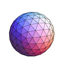
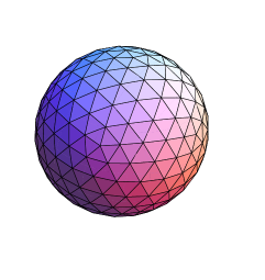
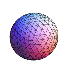
Figure 3. Triangulations of a sphere with 320, 500 and 720 triangles, respectively.

11.4. Scaling a sphere

In section 9 we studied the set of concentric spheres in $n$ dimensions. In dimension three the geodesic equation for the radius simplifies to

$$\boxed{\begin{aligned} r_{tt}&=-r_{t}^{2}\frac{1}{\Phi}\big{[}\frac{1}{r}\Phi+\partial_{v}\Phi 4r^{2}\pi+\frac{1}{r^{2}}(\partial_{\mu}\Phi)+\frac{1}{r^{2}}(\partial_{3}\Phi)\big{]}.\end{aligned}}$$

This equation is in accordance with the numerical results obtained by minimizing the discrete path energy defined in section 11.2. As will be seen, the numerics show that the shortest path connecting two concentric spheres in fact consists of spheres with the same center, and that the above differential equation is (at least qualitatively) satisfied. Furthermore, in our experiments the optimal paths obtained were independent of the initial path used as a starting value for the optimization. In all numerical experiments of this section we used 50 timesteps and a triangulation with 320 triangles.

For conformal metrics of type $\Phi=\operatorname{Vol}^{k}$ and $\Phi=e^{\operatorname{Vol}}$, the ODE for the radius is

$$\Phi=\operatorname{Vol}^{k}: r_{tt}=-r_{t}^{2}\frac{k+1}{r},$$

$$\Phi=e^{\operatorname{Vol}}: r_{tt}=-r_{t}^{2}\Big{(}\frac{1}{r}+4r\pi\Big{)}.$$

Note that the equation for $\Phi=\operatorname{Vol}^{-1}$ is $r_{tt}=0$. These equations have explicit solutions:

$$\Phi=\operatorname{Vol}^{k}: r=C_{1}\big{(}(k+2)t-C_{2}\big{)}^{\frac{1}{k+2}},$$

$$\Phi=e^{\operatorname{Vol}}: r=\frac{1}{2\pi}\sqrt{\log\big{(}C_{1}t+C_{2}\big{)}}.$$

A comparison of the numerical results with the exact analytic solutions can be seen in Figures 5 and 5. The solid lines are the exact solutions. Note that for big radii as in Figure 5, the solution for $\Phi=e^{\operatorname{Vol}}$ has a very steep ascent, is more curved, and lies above the solutions for $\Phi=\operatorname{Vol},\operatorname{Vol}^{2},\operatorname{Vol}^{3}$. For small radii, it lies below these solutions, as can be seen in figure 5. Note also that when the ascent gets too steep, the discrete solution is somewhat inexact as in Figure 5.

\psfrag{Phi1Vol}[cl][cl]{$\Phi=\frac{1}{\operatorname{Vol}}$}\psfrag{PhieVol}[cl][cl]{$\Phi=e^{\operatorname{Vol}}$}\psfrag{PhiVol2}[cl][cl]{$\Phi=\operatorname{Vol}^{2}$}\psfrag{PhiVol3}[cl][cl]{$\Phi=\operatorname{Vol}^{3}$}\psfrag{PhiVol}[cl][cl]{$\Phi=\operatorname{Vol}$}\psfrag{r}[bc][bc]{$r$}\psfrag{t}[cl][cl]{$t$}\psfrag{x0}[tc][tc]{$0$}\psfrag{x11}[tc][tc]{$1$}\psfrag{x1254}[tc][tc]{$1250$}\psfrag{x14}[tc][tc]{$1000$}\psfrag{x154}[tc][tc]{$1500$}\psfrag{x1754}[tc][tc]{$1750$}\psfrag{x21}[tc][tc]{$2$}\psfrag{x253}[tc][tc]{$250$}\psfrag{x2}[tc][tc]{$0.2$}\psfrag{x41}[tc][tc]{$4$}\psfrag{x4}[tc][tc]{$0.4$}\psfrag{x53}[tc][tc]{$500$}\psfrag{x61}[tc][tc]{$6$}\psfrag{x6}[tc][tc]{$0.6$}\psfrag{x753}[tc][tc]{$750$}\psfrag{x81}[tc][tc]{$8$}\psfrag{x8}[tc][tc]{$0.8$}\psfrag{y0}[cr][cr]{$0$}\psfrag{y11}[cr][cr]{$1$}\psfrag{y151}[cr][cr]{$1.5$}\psfrag{y1}[cr][cr]{$0.1$}\psfrag{y21}[cr][cr]{$2$}\psfrag{y2}[cr][cr]{$0.2$}\psfrag{y3}[cr][cr]{$0.3$}\psfrag{y4}[cr][cr]{$0.4$}\psfrag{y5}[cr][cr]{$0.5$}\psfrag{y6}[cr][cr]{$0.6$}\psfrag{y7}[cr][cr]{$0.7$}\psfrag{y8}[cr][cr]{$0.8$}\psfrag{ym11}[cr][cr]{$-1$}\psfrag{ym1253}[cr][cr]{$-125$}\psfrag{ym13}[cr][cr]{$-100$}\psfrag{ym151}[cr][cr]{$-1.5$}\psfrag{ym153}[cr][cr]{$-150$}\psfrag{ym21}[cr][cr]{$-2$}\psfrag{ym252}[cr][cr]{$-25$}\psfrag{ym52}[cr][cr]{$-50$}\psfrag{ym5}[cr][cr]{$-0.5$}\psfrag{ym752}[cr][cr]{$-75$}\includegraphics[width=312.20692pt]{scale_00_scale_conformal_bigradius}

Figure 4. Geodesics between concentric spheres of radius $0.4$ to $0.8$ for several conformal metrics. Solid lines are the exact solutions.

\psfrag{Phi1Vol}[cl][cl]{$\Phi=\frac{1}{\operatorname{Vol}}$}\psfrag{PhieVol}[cl][cl]{$\Phi=e^{\operatorname{Vol}}$}\psfrag{PhiVol2}[cl][cl]{$\Phi=\operatorname{Vol}^{2}$}\psfrag{PhiVol3}[cl][cl]{$\Phi=\operatorname{Vol}^{3}$}\psfrag{PhiVol}[cl][cl]{$\Phi=\operatorname{Vol}$}\psfrag{r}[bc][bc]{$r$}\psfrag{t}[cl][cl]{$t$}\psfrag{x0}[tc][tc]{$0$}\psfrag{x11}[tc][tc]{$1$}\psfrag{x1254}[tc][tc]{$1250$}\psfrag{x14}[tc][tc]{$1000$}\psfrag{x154}[tc][tc]{$1500$}\psfrag{x1754}[tc][tc]{$1750$}\psfrag{x21}[tc][tc]{$2$}\psfrag{x253}[tc][tc]{$250$}\psfrag{x2}[tc][tc]{$0.2$}\psfrag{x41}[tc][tc]{$4$}\psfrag{x4}[tc][tc]{$0.4$}\psfrag{x53}[tc][tc]{$500$}\psfrag{x61}[tc][tc]{$6$}\psfrag{x6}[tc][tc]{$0.6$}\psfrag{x753}[tc][tc]{$750$}\psfrag{x81}[tc][tc]{$8$}\psfrag{x8}[tc][tc]{$0.8$}\psfrag{y0}[cr][cr]{$0$}\psfrag{y11}[cr][cr]{$1$}\psfrag{y12}[cr][cr]{$0.12$}\psfrag{y14}[cr][cr]{$0.14$}\psfrag{y151}[cr][cr]{$1.5$}\psfrag{y16}[cr][cr]{$0.16$}\psfrag{y18}[cr][cr]{$0.18$}\psfrag{y1}[cr][cr]{$0.1$}\psfrag{y21}[cr][cr]{$2$}\psfrag{y2}[cr][cr]{$0.2$}\psfrag{y3}[cr][cr]{$0.3$}\psfrag{y4}[cr][cr]{$0.4$}\psfrag{y5}[cr][cr]{$0.5$}\psfrag{y6}[cr][cr]{$0.6$}\psfrag{ym11}[cr][cr]{$-1$}\psfrag{ym1253}[cr][cr]{$-125$}\psfrag{ym13}[cr][cr]{$-100$}\psfrag{ym151}[cr][cr]{$-1.5$}\psfrag{ym153}[cr][cr]{$-150$}\psfrag{ym21}[cr][cr]{$-2$}\psfrag{ym252}[cr][cr]{$-25$}\psfrag{ym52}[cr][cr]{$-50$}\psfrag{ym5}[cr][cr]{$-0.5$}\psfrag{ym752}[cr][cr]{$-75$}\includegraphics[width=312.20692pt]{scale_00_scale_conformal_smallradius}

Figure 5. Geodesics between concentric spheres of radius $0.1$ to $0.2$ for several conformal metrics. Solid lines are the exact solutions.

\psfrag{k2}[cl][cl]{$k=2$}\psfrag{k4}[cl][cl]{$k=4$}\psfrag{k6}[cl][cl]{$k=6$}\psfrag{k8}[cl][cl]{$k=8$}\psfrag{r}[bc][bc]{$r$}\psfrag{t}[cl][cl]{$t$}\psfrag{x0}[tc][tc]{$0$}\psfrag{x11}[tc][tc]{$1$}\psfrag{x124}[tc][tc]{$1200$}\psfrag{x144}[tc][tc]{$1400$}\psfrag{x14}[tc][tc]{$1000$}\psfrag{x21}[tc][tc]{$2$}\psfrag{x23}[tc][tc]{$200$}\psfrag{x2}[tc][tc]{$0.2$}\psfrag{x41}[tc][tc]{$4$}\psfrag{x43}[tc][tc]{$400$}\psfrag{x4}[tc][tc]{$0.4$}\psfrag{x61}[tc][tc]{$6$}\psfrag{x63}[tc][tc]{$600$}\psfrag{x6}[tc][tc]{$0.6$}\psfrag{x81}[tc][tc]{$8$}\psfrag{x83}[tc][tc]{$800$}\psfrag{x8}[tc][tc]{$0.8$}\psfrag{y0}[cr][cr]{$0$}\psfrag{y11}[cr][cr]{$1$}\psfrag{y121}[cr][cr]{$1.2$}\psfrag{y141}[cr][cr]{$1.4$}\psfrag{y151}[cr][cr]{$1.5$}\psfrag{y161}[cr][cr]{$1.6$}\psfrag{y181}[cr][cr]{$1.8$}\psfrag{y1}[cr][cr]{$0.1$}\psfrag{y21}[cr][cr]{$2$}\psfrag{y2}[cr][cr]{$0.2$}\psfrag{y3}[cr][cr]{$0.3$}\psfrag{y4}[cr][cr]{$0.4$}\psfrag{y5}[cr][cr]{$0.5$}\psfrag{y6}[cr][cr]{$0.6$}\psfrag{ym11}[cr][cr]{$-1$}\psfrag{ym1253}[cr][cr]{$-125$}\psfrag{ym13}[cr][cr]{$-100$}\psfrag{ym151}[cr][cr]{$-1.5$}\psfrag{ym153}[cr][cr]{$-150$}\psfrag{ym21}[cr][cr]{$-2$}\psfrag{ym252}[cr][cr]{$-25$}\psfrag{ym52}[cr][cr]{$-50$}\psfrag{ym5}[cr][cr]{$-0.5$}\psfrag{ym752}[cr][cr]{$-75$}\includegraphics[width=312.20692pt]{scale_00_scale_ga_varyingk}

Figure 6. Geodesics between concentric spheres for $\Phi=1+0.1\operatorname{Tr}(L)^{k}$ and varying $k$. Solid lines are the exact solutions.

\psfrag{A001}[cl][cl]{$A=0.01$}\psfrag{A01}[cl][cl]{$A=0.1$}\psfrag{A0}[cl][cl]{$A=0$}\psfrag{A1}[cl][cl]{$A=1$}\psfrag{r}[bc][bc]{$r$}\psfrag{t}[cl][cl]{$t$}\psfrag{x0}[tc][tc]{$0$}\psfrag{x11}[tc][tc]{$1$}\psfrag{x124}[tc][tc]{$1200$}\psfrag{x144}[tc][tc]{$1400$}\psfrag{x14}[tc][tc]{$1000$}\psfrag{x21}[tc][tc]{$2$}\psfrag{x23}[tc][tc]{$200$}\psfrag{x2}[tc][tc]{$0.2$}\psfrag{x41}[tc][tc]{$4$}\psfrag{x43}[tc][tc]{$400$}\psfrag{x4}[tc][tc]{$0.4$}\psfrag{x61}[tc][tc]{$6$}\psfrag{x63}[tc][tc]{$600$}\psfrag{x6}[tc][tc]{$0.6$}\psfrag{x81}[tc][tc]{$8$}\psfrag{x83}[tc][tc]{$800$}\psfrag{x8}[tc][tc]{$0.8$}\psfrag{y0}[cr][cr]{$0$}\psfrag{y11}[cr][cr]{$1$}\psfrag{y151}[cr][cr]{$1.5$}\psfrag{y1}[cr][cr]{$0.1$}\psfrag{y21}[cr][cr]{$2$}\psfrag{y2}[cr][cr]{$0.2$}\psfrag{y3}[cr][cr]{$0.3$}\psfrag{y4}[cr][cr]{$0.4$}\psfrag{y5}[cr][cr]{$0.5$}\psfrag{y6}[cr][cr]{$0.6$}\psfrag{y8}[cr][cr]{$0.8$}\psfrag{ym11}[cr][cr]{$-1$}\psfrag{ym1253}[cr][cr]{$-125$}\psfrag{ym13}[cr][cr]{$-100$}\psfrag{ym151}[cr][cr]{$-1.5$}\psfrag{ym153}[cr][cr]{$-150$}\psfrag{ym21}[cr][cr]{$-2$}\psfrag{ym252}[cr][cr]{$-25$}\psfrag{ym52}[cr][cr]{$-50$}\psfrag{ym5}[cr][cr]{$-0.5$}\psfrag{ym752}[cr][cr]{$-75$}\includegraphics[width=312.20692pt]{scale_00_scale_ga_varyinga}

Figure 7. Geodesics between concentric spheres for $\Phi=1+A\operatorname{Tr}(L)^{2}$ and varying $A$. Solid lines are the exact solutions.

\psfrag{Phisi}[cl][cl]{$\Phi={\operatorname{Vol}^{-2}}+A\operatorname{Tr}(L)^{2}\operatorname{Vol}^{-1}$}\psfrag{r}[bc][bc]{$r$}\psfrag{t}[cl][cl]{$t$}\psfrag{x0}[tc][tc]{$0$}\psfrag{x11}[tc][tc]{$1$}\psfrag{x12}[tc][tc]{$10$}\psfrag{x13}[tc][tc]{$100$}\psfrag{x152}[tc][tc]{$15$}\psfrag{x153}[tc][tc]{$150$}\psfrag{x22}[tc][tc]{$20$}\psfrag{x23}[tc][tc]{$200$}\psfrag{x252}[tc][tc]{$25$}\psfrag{x253}[tc][tc]{$250$}\psfrag{x2}[tc][tc]{$0.2$}\psfrag{x33}[tc][tc]{$300$}\psfrag{x353}[tc][tc]{$350$}\psfrag{x4}[tc][tc]{$0.4$}\psfrag{x51}[tc][tc]{$5$}\psfrag{x52}[tc][tc]{$50$}\psfrag{x6}[tc][tc]{$0.6$}\psfrag{x8}[tc][tc]{$0.8$}\psfrag{y0}[cr][cr]{$0$}\psfrag{y11}[cr][cr]{$1$}\psfrag{y12}[cr][cr]{$0.12$}\psfrag{y14}[cr][cr]{$0.14$}\psfrag{y151}[cr][cr]{$1.5$}\psfrag{y16}[cr][cr]{$0.16$}\psfrag{y18}[cr][cr]{$0.18$}\psfrag{y1}[cr][cr]{$0.1$}\psfrag{y21}[cr][cr]{$2$}\psfrag{y2}[cr][cr]{$0.2$}\psfrag{y3}[cr][cr]{$0.3$}\psfrag{y4}[cr][cr]{$0.4$}\psfrag{y5}[cr][cr]{$0.5$}\psfrag{y6}[cr][cr]{$0.6$}\psfrag{ym11}[cr][cr]{$-1$}\psfrag{ym12}[cr][cr]{$-10$}\psfrag{ym151}[cr][cr]{$-1.5$}\psfrag{ym21}[cr][cr]{$-2$}\psfrag{ym22}[cr][cr]{$-20$}\psfrag{ym32}[cr][cr]{$-30$}\psfrag{ym42}[cr][cr]{$-40$}\psfrag{ym52}[cr][cr]{$-50$}\psfrag{ym5}[cr][cr]{$-0.5$}\includegraphics[width=312.20692pt]{scale_00_scale_si}

Figure 8. Geodesics between concentric spheres for the scale-invariant metric.

For mean curvature weighted metrics, the differential equation for the radius is

$$\Phi=1+A\operatorname{Tr}(L)^{2k}: r_{tt}=-r_{t}^{2}\Big{(}\frac{1}{r}-\frac{2kA2^{2k-1}}{r^{2k+1}+A2^{2k}r}\Big{)}.$$

The numerics for these metrics are shown in figure 7 and figure 7. Note that we got convergence to a path consisting of concentric spheres even for the $G^{0}$-metric ($A=0$), even though we know from the theory that this is not the shortest path. In fact, there are no shortest paths for the $G^{0}$–metric since it has vanishing geodesic distance [14].

For the scale-invariant metric, the differential equation is given by

$$\Phi=\operatorname{Vol}^{-2}+A\frac{\operatorname{Tr}(L)^{2}}{\operatorname{Vol}}: r_{tt}=\frac{r_{t}^{2}}{r}.$$

This equation has an explicit analytical solution

$$\Phi=\operatorname{Vol}^{-2}+A\frac{\operatorname{Tr}(L)^{2}}{\operatorname{Vol}}: r=C_{1}e^{C_{2}t}.$$

Note that this equation, and therefore its solution, is independent of $A$. Again, this is confirmed by the numerics: see Figure 8.

11.5. Translation of a sphere

In this section we will study geodesics between a sphere and a translated sphere for various almost local metrics of the type $\Phi=\operatorname{Vol}^{k}$, $\Phi=e^{\operatorname{Vol}}$, and $\Phi=1+A\operatorname{Tr}(L)^{2k}$.

Depending on the distance (relative to the radius) of the two translated spheres, different behaviors can be observed.

High distance:

• Shrink and grow: For some metrics it is possible to shrink a sphere in finite time to zero. For these metrics long translation goes via a shrinking part and growing part. Metrics with this behavior are $\Phi=\operatorname{Vol}^{k}$, $\Phi=e^{\operatorname{Vol}}$ and $\Phi=1+A\operatorname{Tr}(L)^{2}$. This phenomenon is studied in more detail in section 11.6; see also Figure 10.

• Moving an optimal middle shape: For some of the metrics translation of a sphere with a certain optimal radius is a geodesic. For these metrics geodesics for long translations scale the sphere to the optimal radius and translate the sphere with the optimal radius. Metrics with this behavior are $\Phi=1+A\operatorname{Tr}(L)^{2k}$ for $k>1$. This behavior is studied in section 11.7.

Low distance:

• Geodesics of pure translation ($\Phi=1+A\operatorname{Tr}(L)^{2k}$ for $k>1$; c.f. Figure 13).

• Geodesics that pass through an ellipsoid, where the longer principal axis is in the direction of the translation (conformal metrics, c.f. Figure 9).

• Geodesics that pass through an ellipsoid, where the principal axis in the direction of the translation is shorter ($\Phi=1+A\operatorname{Tr}(L)^{2k}$ for $k>1$, c.f. Figure 13).

• Geodesics that pass through a cigar–shaped figure ($\Phi=1+A\operatorname{Tr}(L)^{2},$ c.f. Figure 12).

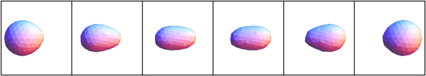
Figure 9. Geodesic between two unit spheres translated by distance $1.5$ for $\Phi=\operatorname{Vol}$. 20 timesteps and a triangulation with 500 triangles were used. Time progresses from left to right. Boundary shapes $t=0$ and $t=1$ are not included.

11.6. Shrink and grow

In section 9 we showed that it is possible to shrink a sphere to zero in finite time for some of the metrics, namely, conformal metrics with $\Phi=\operatorname{Vol}^{k}$ or $\Phi=e^{\operatorname{Vol}}$ and for the $G^{A}$–metric. For these metrics geodesics of long translation will go via a shrinking part and growing part, and almost all of the translation will be done with the shrunken version of the shape. An example of such a geodesic can be seen in figure 10.

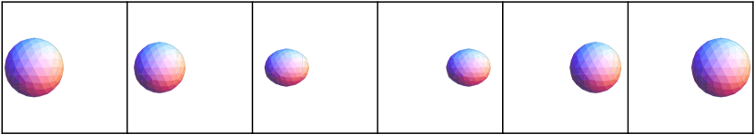
Figure 10. Geodesic between two unit spheres translated by distance $2$ for $\Phi=e^{\operatorname{Vol}}$. 20 timesteps and a triangulation with 500 triangles were used. Time progresses from left to right. Boundary shapes $t=0$ and $t=1$ are not included.

We could not determine numerically whether a collapse of the sphere to a point occurs or not. But the more time steps were used, the smaller the ellipsoid in the middle turned out. Also, the energy of the geodesic path comes very close to the energy needed to shrink the sphere to a point and blow it up again. It is remarkable that almost all of the translation is concentrated at a single time step, independently of the number of timesteps that were used. The reason for this behavior is that high volumes are penalized so much: In the case of figure 10, $e^{\operatorname{Vol}}$ is more than 1000 times smaller in the middle than at the boundary shapes.

We now want find out under what conditions on the distance and radius of the boundary spheres of the geodesic this behavior can occur. To do this, we compare the energy needed for a pure translation with the energy needed to first shrink the sphere to almost zero, then move it, and then blow it up again.

The energy needed for a pure translation of a sphere with radius $r$ by distance $\ell$ in the direction of a unit vector $e_{1}$ is given by

$$E =\int_{0}^{1}\int_{S^{2}}\Phi(\operatorname{Vol},\operatorname{Tr}(L))\bar{g}(\ell.e_{1},\nu)^{2}\operatorname{vol}(g)dt$$

$$=\Phi(4r^{2}\pi,-\frac{2}{r})\int_{0}^{\pi}\int_{0}^{2\pi}\bar{g}\left(\ell.e_{1},\left(\begin{array}[]{c}\cos\varphi\sin\theta\\ \sin\varphi\sin\theta\\ \cos\theta\end{array}\right)\right)^{2}r^{2}\sin\theta\ d\varphi d\theta$$

$$=\Phi(4r^{2}\pi,-\frac{2}{r})\int_{0}^{\pi}\int_{0}^{2\pi}\ell^{2}.(\cos\varphi\sin\theta)^{2}r^{2}\sin\theta d\varphi d\theta=\Phi(4r^{2}\pi,-\frac{2}{r}).\frac{4\pi}{3}\ell^{2}.r^{2}.$$

Any other unit vector can be chosen instead of $e_{1}$, yielding the same result.

\psfrag{l}[bc][bc]{$l$}\psfrag{Phi1TrL2}[cl][cl]{$G^{1}$}\psfrag{PhieVol}[cl][cl]{$\Phi=e^{\operatorname{Vol}}$}\psfrag{PhiVol2}[cl][cl]{$\Phi=\operatorname{Vol}^{2}$}\psfrag{PhiVol3}[cl][cl]{$\Phi=\operatorname{Vol}^{3}$}\psfrag{PhiVol}[cl][cl]{$\Phi=\operatorname{Vol}$}\psfrag{rA}[cl][cl]{$r$}\psfrag{r}[bc][bc]{$r$}\psfrag{t}[cl][cl]{$t$}\psfrag{x00}[tc][tc]{$0.0$}\psfrag{x05}[tc][tc]{$0.5$}\psfrag{x0}[tc][tc]{$0$}\psfrag{x10}[tc][tc]{$1.0$}\psfrag{x11}[tc][tc]{$1$}\psfrag{x1254}[tc][tc]{$1250$}\psfrag{x12}[tc][tc]{$10$}\psfrag{x14}[tc][tc]{$1000$}\psfrag{x154}[tc][tc]{$1500$}\psfrag{x15}[tc][tc]{$1.5$}\psfrag{x1754}[tc][tc]{$1750$}\psfrag{x21}[tc][tc]{$2$}\psfrag{x253}[tc][tc]{$250$}\psfrag{x2}[tc][tc]{$0.2$}\psfrag{x41}[tc][tc]{$4$}\psfrag{x4}[tc][tc]{$0.4$}\psfrag{x53}[tc][tc]{$500$}\psfrag{x61}[tc][tc]{$6$}\psfrag{x6}[tc][tc]{$0.6$}\psfrag{x753}[tc][tc]{$750$}\psfrag{x81}[tc][tc]{$8$}\psfrag{x8}[tc][tc]{$0.8$}\psfrag{y00}[cr][cr]{$0.0$}\psfrag{y05}[cr][cr]{$0.5$}\psfrag{y0}[cr][cr]{$0$}\psfrag{y10}[cr][cr]{$1.0$}\psfrag{y11}[cr][cr]{$1$}\psfrag{y151}[cr][cr]{$1.5$}\psfrag{y1}[cr][cr]{$0.1$}\psfrag{y21}[cr][cr]{$2$}\psfrag{y2}[cr][cr]{$0.2$}\psfrag{y3}[cr][cr]{$0.3$}\psfrag{y4}[cr][cr]{$0.4$}\psfrag{y5}[cr][cr]{$0.5$}\psfrag{y6}[cr][cr]{$0.6$}\psfrag{y8}[cr][cr]{$0.8$}\psfrag{ym11}[cr][cr]{$-1$}\psfrag{ym123}[cr][cr]{$-120$}\psfrag{ym13}[cr][cr]{$-100$}\psfrag{ym151}[cr][cr]{$-1.5$}\psfrag{ym21}[cr][cr]{$-2$}\psfrag{ym22}[cr][cr]{$-20$}\psfrag{ym42}[cr][cr]{$-40$}\psfrag{ym5}[cr][cr]{$-0.5$}\psfrag{ym62}[cr][cr]{$-60$}\psfrag{ym82}[cr][cr]{$-80$}\includegraphics[width=433.62pt]{move_sphere_01_conformal_varying_distance_00_shrink_n_blow}

Figure 11. Left: Shrinking a sphere to zero along a geodesic path and blowing it up again. Right: Pairs of $\ell$ and $r$ such that translating a sphere of radius $r$ by distance $\ell$ needs as much energy as shrinking it to zero and blowing it up again. $G^{1}$ stands for the $G^{A}$ metric with $A=1$.

We will now calculate the energy needed for shrinking the sphere, moving it, and blowing it up again. The energy needed for translating a sphere of radius almost zero can be neglected. Shrinking and blowing up are done using the solutions to the geodesic equation for the radius from the last section, where one has to adapt the constants to the boundary conditions. For the shrinking part we have $r(0)=r$ and $r(\tfrac{1}{2})=0$, and for the growing part we have $r(\tfrac{1}{2})=0,r(1)=r$; see Figure 11 (left).

The energy of the path is

$$\Phi=\operatorname{Vol}^{k}: E=\int_{0}^{1}\operatorname{Vol}^{k}\int_{S^{2}}r_{t}^{2}\operatorname{vol}(g)dt=\frac{4^{k+2}\pi^{k+1}}{(k+2)^{2}}r^{2k+4},$$

$$\Phi=e^{\operatorname{Vol}}: E=\int_{0}^{1}e^{\operatorname{Vol}}\int_{S^{2}}r_{t}^{2}\operatorname{vol}(g)dt=\frac{1}{\pi}(e^{2\pi r^{2}}-1)^{2}.$$

The energy of the two different paths are the same when

$$\Phi=\operatorname{Vol}^{k}: \ell=\frac{2\sqrt{3}r}{k+2},$$

$$\Phi=e^{\operatorname{Vol}}: \ell=\frac{\sqrt{3}(1-e^{-2\pi r^{2}})}{2r\pi}.$$

These curves are shown in Figure  11 (right). We did not derive an analytic solution for the $G^{A}$–metric, but for $A=1$ one can see the solution curves in figure 11.

11.7. Moving an optimal shape

In the following we want to determine whether pure translation of a sphere is a geodesic. Therefore, let $f_{t}=f_{0}+b(t)\cdot e_{1}$, where $f_{0}$ is a sphere of radius $r$ and where $b(t)$ is constant on $M$. Plugging this into the geodesic equation from section 5.1 yields an ODE for $b(t)$ and a part which has to vanish identically. The latter is given by

(1) $$(\partial_{v}\Phi)\frac{2}{r}4r^{2}\pi+(\partial_{\mu}\Phi)\frac{2}{r^{2}}+\Phi\frac{2}{r}=0$$

For conformal metrics this equation is satisfied only if $\Phi=\operatorname{Vol}^{-1}$. Since this metric induces vanishing geodesic distance (see section 8) we are not interested in this case. For curvature weighted metrics the above equation reads as

$$\Phi =1+A\operatorname{Tr}(L)^{2k}:\qquad\frac{4^{k}A(k-1)}{r^{4k}}=1$$

Solutions to these equations are given by

$$\Phi =1+A\operatorname{Tr}(L)^{2k}:\qquad r=2\sqrt[2k]{A(k-1)},\quad k\geq 1.$$

For the most prominent example, the $G^{A}$–metric, this yields $r=0$, and therefore translation can never be a geodesic for this type of metric. The numerics have shown that the $G^{A}$–metric yields geodesics that resemble the geodesics of the $G^{A}$–metric for planar curves from [15, section 5.2]. Namely, when the two spheres are sufficiently far apart, the geodesic passes through a cigar-like middle shape, see figure 12. As predicted by the theory (see section 8.9), geodesics for very high distances tend to have behavior similar to that of $\operatorname{Vol}^{k}$ metrics; i.e., the geodesic first shrinks the sphere, then moves it, and then blows it up again (cf. section 11.6).

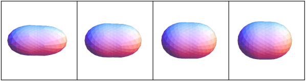
Figure 12. Middle figure of a geodesic between two unit spheres translated by distance $3$ for $\Phi=1+A\operatorname{Tr}(L)^{2}$. From left to right: $A=0.2$, $A=0.4$, $A=0.6$, $A=0.8$. In each of the simulations 20 timesteps and a triangulation with 720 triangles were used.

For metrics weighted by higher factors of mean curvature, the above equation for the radius has a positive solution. For these metrics, geodesics for translations tend to scale the sphere until it has reached the optimal radius and then translate it. If the radius is already optimal, the resulting geodesic is a pure translation (see figure 13).

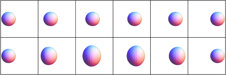
Figure 13. Geodesic between two unit spheres translated by distance $3$ for $\Phi=1+\frac{1}{16}\operatorname{Tr}(L)^{4}$ (first row) and $\Phi=1+\operatorname{Tr}(L)^{6}$ (second row). In each of the experiments 20 timesteps and a triangulation with 720 triangles were used. Time progresses from left to right. Boundary shapes $t=0$ and $t=1$ are not included.

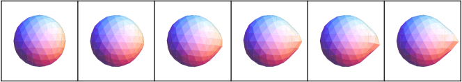
Figure 14. Geodesic between a sphere and a sphere with a small bump for $\Phi=\operatorname{Vol}$. 20 timesteps and a triangulation with 500 triangles were used. Time progresses from left to right.

If the distance is not high enough a scaling towards the optimal size still occurs, but the middle figure is not a perfect sphere anymore. Instead it is an ellipsoid as in figure 13.

11.8. Deformation of a shape

We will calculate numerically the geodesic between a shape and a deformation of the shape for various almost local metrics. Small deformations are handled well by all metrics, and they all yield similar results. An example of a geodesic resulting in a small deformation can be seen in figure 14, where a small bump is grown out of a sphere. The energy needed for this deformation is reasonable compared to the energy needed for a pure translation. Taking the metric with $\Phi=\operatorname{Vol}$ as an example, growing a bump of size 0.4 as in figure 14 costs about a third of a translation of the sphere by 0.4.

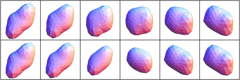
Figure 15. Large deformation of a shape for $\Phi=\operatorname{Vol}$ and $\Phi=e^{\operatorname{Vol}}$. 20 timesteps and a triangulation with 500 triangles were used. Time progresses from left to right.

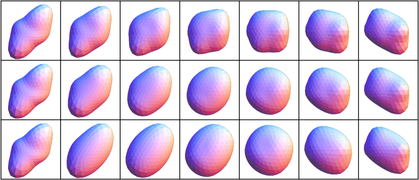
Figure 16. Large deformation of a shape for $\Phi=1+0.1\operatorname{Tr}(L)^{2}$ (top), $\Phi=1+10\operatorname{Tr}(L)^{2}$ (middle), and $\Phi=1+\operatorname{Tr}(L)^{6}$ (bottom). 20 timesteps and a triangulation with 720 triangles were used. Time progresses from left to right.

Bigger deformations work well with $\operatorname{Vol}^{k}$-metrics and curvature weighted metrics, but not with the $e^{\operatorname{Vol}}$-metric, which tends to shrink the object and to concentrate almost all of the deformation at a single time step. In figure 15, a large deformation can be seen for the case of $\Phi=\operatorname{Vol}$ and $\Phi=e^{\operatorname{Vol}}$. Clearly one can see that the $e^{\operatorname{Vol}}$-metric concentrates almost all of the deformation in a single time step. We have met this misbehavior of the $e^{\operatorname{Vol}}$-metric already with translations. Again, the reason is that $e^{\operatorname{Vol}}$ is so sensitive to changes in volume. In figure 16 one sees that geodesics are smoothed further by higher curvature weights.

The AMPL model file

Listing 1: AMPL model file

⬇

1param A default 1;

param k default 1;

3param B default 1;

param l default 1;

5param TimestepsN > 1 integer;

param VerticesN integer;

7param PenaltyFactor default 1;

param PenaltyExponent default 2;

9set VerticesI := 1..VerticesN;

set VerticesOfEdgesI within {VerticesI,VerticesI};

11set VerticesOfFacesI within {VerticesI,VerticesI,VerticesI};

set FacesOfVerticesI {v in VerticesI} within VerticesOfFacesI;

13set LinkOfVerticesI {VerticesI} within {VerticesOfFacesI,VerticesOfEdgesI,{-1,1}};

set AdjacentEdgesOfVerticesI {VerticesI} within {VerticesOfEdgesI,{1,-1},VerticesOfEdgesI,{1,-1}};

15set EdgesOfFacesI {VerticesOfFacesI} within VerticesOfEdgesI;

set EdgesOfVerticesI {v in VerticesI} := setof {(f1,f2,f3,e1,e2,o) in LinkOfVerticesI[v]}(e1,e2);

17

param Pi default 3.141592653589793;

19param PerfectAngle {v in VerticesI} default cos(2*Pi/card(FacesOfVerticesI[v]));

param InitialVertices {VerticesI,1..3};

21param FinalVertices {VerticesI,1..3};

23var MiddleVertices {2..TimestepsN,VerticesI,1..3};

25var Vertices {t in 1..TimestepsN+1,v in VerticesI,i in 1..3} =

(if t=1 then InitialVertices[v,i]

27 else if t=TimestepsN+1 then FinalVertices[v,i]

else MiddleVertices[t,v,i]);

29

var VectorOfEdges {t in 1..TimestepsN+1, (v1,v2) in VerticesOfEdgesI,i in 1..3} =

31 Vertices[t,v2,i] - Vertices[t,v1,i];

33var LengthOfEdges {t in 1..TimestepsN+1, (v1,v2) in VerticesOfEdgesI} =

sqrt(VectorOfEdges[t,v1,v2,1]^2+VectorOfEdges[t,v1,v2,2]^2+VectorOfEdges[t,v1,v2,3]^2);

35

var CrossOfFaces {t in 1..TimestepsN+1,(v1,v2,v3) in VerticesOfFacesI,i in 1..3} =

37 if i=1 then (Vertices[t,v2,2]-Vertices[t,v1,2])*(Vertices[t,v3,3]-Vertices[t,v1,3]) -

(Vertices[t,v2,3]-Vertices[t,v1,3])*(Vertices[t,v3,2]-Vertices[t,v1,2])

39 else if i=2 then -(Vertices[t,v2,1]-Vertices[t,v1,1])*(Vertices[t,v3,3]-Vertices[t,v1,3]) +

(Vertices[t,v2,3]-Vertices[t,v1,3])*(Vertices[t,v3,1]-Vertices[t,v1,1])

41 else (Vertices[t,v2,1]-Vertices[t,v1,1])*(Vertices[t,v3,2]-Vertices[t,v1,2]) -

(Vertices[t,v2,2]-Vertices[t,v1,2])*(Vertices[t,v3,1]-Vertices[t,v1,1]) ;

43

var NormCrossOfFaces {t in 1..TimestepsN+1,(v1,v2,v3) in VerticesOfFacesI} =

45 sqrt(CrossOfFaces[t,v1,v2,v3,1]^2 + CrossOfFaces[t,v1,v2,v3,2]^2 + CrossOfFaces[t,v1,v2,v3,3]^2);

47var NuOfFaces {t in 1..TimestepsN+1,(v1,v2,v3) in VerticesOfFacesI,i in 1..3} =

CrossOfFaces[t,v1,v2,v3,i]/NormCrossOfFaces[t,v1,v2,v3];

49

var AreaOfFaces {t in 1..TimestepsN+1,(v1,v2,v3) in VerticesOfFacesI} =

51 NormCrossOfFaces[t,v1,v2,v3]/2;

53var AreaOfVertices {t in 1..TimestepsN+1, v in VerticesI} =

(sum {(f1,f2,f3) in FacesOfVerticesI[v]} AreaOfFaces[t,f1,f2,f3])/3;

55

var VectorAreaOfVertices {t in 1..TimestepsN+1, v in VerticesI, i in 1..3} =

57 (sum {(v1,v2,v3) in FacesOfVerticesI[v]} CrossOfFaces[t,v1,v2,v3,i])/6;

59var SquareOfNormOfVectorAreaOfVertices {t in 1..TimestepsN+1, v in VerticesI} =

VectorAreaOfVertices[t,v,1]^2+VectorAreaOfVertices[t,v,2]^2+VectorAreaOfVertices[t,v,3]^2;

61

var NormOfVectorAreaOfVertices {t in 1..TimestepsN+1, v in VerticesI} =

63 sqrt( SquareOfNormOfVectorAreaOfVertices[t,v]);

65var Volume {t in 1..TimestepsN+1} =

sum{(v1,v2,v3) in VerticesOfFacesI} AreaOfFaces[t,v1,v2,v3];

67

var VectorMeanCurvatureOfVertices {t in 1..TimestepsN+1, v in VerticesI, i in 1..3} =

69 if i=1 then

sum {(f1,f2,f3,e1,e2,o) in LinkOfVerticesI[v]} o*

71 ( VectorOfEdges[t,e1,e2,2]*NuOfFaces[t,f1,f2,f3,3] -

VectorOfEdges[t,e1,e2,3]*NuOfFaces[t,f1,f2,f3,2] )

73 else if i=2 then

sum {(f1,f2,f3,e1,e2,o) in LinkOfVerticesI[v]} o*

75 (-VectorOfEdges[t,e1,e2,1]*NuOfFaces[t,f1,f2,f3,3] +

VectorOfEdges[t,e1,e2,3]*NuOfFaces[t,f1,f2,f3,1] )

77 else

sum {(f1,f2,f3,e1,e2,o) in LinkOfVerticesI[v]} o*

79 ( VectorOfEdges[t,e1,e2,1]*NuOfFaces[t,f1,f2,f3,2] -

VectorOfEdges[t,e1,e2,2]*NuOfFaces[t,f1,f2,f3,1] ) ;

81

var SquareOfScalarMeanCurvatureOfVertices {t in 1..TimestepsN+1, v in VerticesI} =

83 (VectorMeanCurvatureOfVertices[t,v,1]^2+VectorMeanCurvatureOfVertices[t,v,2]^2

+VectorMeanCurvatureOfVertices[t,v,3]^2)/SquareOfNormOfVectorAreaOfVertices[t,v];

85

var PhiOfVertices {t in 1..TimestepsN+1,v in VerticesI} =

87 1+ A*(SquareOfScalarMeanCurvatureOfVertices[t,v])^k +B*(Volume[t])^l;

89var IncrementsOfVertices {t in 1..TimestepsN,v in VerticesI,i in 1..3} =

TimestepsN*(Vertices[t+1,v,i] - Vertices[t,v,i]);

91

var Energy = 1/ 12 / TimestepsN *(

93 sum {t in 1..TimestepsN,v in VerticesI}

PhiOfVertices[t,v] * sum {(w1,w2,w3) in FacesOfVerticesI[v]}

95 ( IncrementsOfVertices[t,v,1]*CrossOfFaces[t,w1,w2,w3,1] +

IncrementsOfVertices[t,v,2]*CrossOfFaces[t,w1,w2,w3,2] +

97 IncrementsOfVertices[t,v,3]*CrossOfFaces[t,w1,w2,w3,3] )^2 /

NormCrossOfFaces[t,w1,w2,w3] +

99 sum {t in 1..TimestepsN,v in VerticesI}

PhiOfVertices[t+1,v] * sum {(w1,w2,w3) in FacesOfVerticesI[v]}

101 ( IncrementsOfVertices[t,v,1]*CrossOfFaces[t+1,w1,w2,w3,1] +

IncrementsOfVertices[t,v,2]*CrossOfFaces[t+1,w1,w2,w3,2] +

103 IncrementsOfVertices[t,v,3]*CrossOfFaces[t+1,w1,w2,w3,3] )^2 /

NormCrossOfFaces[t+1,w1,w2,w3] );

105

var Penalty =

107 sum {t in 1..TimestepsN+1, v in VerticesI,(v1,w1,o1,v2,w2,o2) in AdjacentEdgesOfVerticesI[v]}

abs(

109 ( VectorOfEdges[t,v1,w1,1]*VectorOfEdges[t,v2,w2,1] +

VectorOfEdges[t,v1,w1,2]*VectorOfEdges[t,v2,w2,2] +

111 VectorOfEdges[t,v1,w1,3]*VectorOfEdges[t,v2,w2,3] ) * o1 * o2

/ LengthOfEdges[t,v1,w1] / LengthOfEdges[t,v2,w2]

113 - PerfectAngle[v]

)^PenaltyExponent;

115

minimize f:

117 Energy+Penalty*PenaltyFactor;

References

- [1] M. Bauer, P. Harms, and P. W. Michor. Curvature weighted metrics on shape space of hypersurfaces in n-space. To appear in: Differential Geometry and its Applications. arXiv:1102.0678.
- [2] M. Bauer, P. Harms, and P. W. Michor. Sobolev metrics on shape space of surfaces in n-space. To appear in: Journal of Geometric Mechanics. arXiv:1009.3616.
- [3] Martin Bauer. Almost local metrics on shape space of surfaces. PhD thesis, University of Vienna, 2010.
- [4] Arthur L. Besse. Einstein manifolds. Classics in Mathematics. Springer-Verlag, Berlin, 2008.
- [5] V. Cervera, F. Mascaró, and P. W. Michor. The action of the diffeomorphism group on the space of immersions. Differential Geom. Appl., 1(4):391–401, 1991.
- [6] R. Fourer and B. W. Kernighan. AMPL: A Modeling Language for Mathematical Programming. Duxbury Press, 2002.
- [7] William Fulton. Young tableaux, volume 35 of London Mathematical Society Student Texts. Cambridge University Press, 1997.
- [8] Philipp Harms. Sobolev metrics on shape space of surfaces. PhD thesis, University of Vienna, 2010.
- [9] Shoshichi Kobayashi and Katsumi Nomizu. Foundations of differential geometry. Vol. I. Wiley Classics Library. John Wiley & Sons Inc., New York, 1996.
- [10] I. Kolávr, P. W. Michor, and J. Slovák. Natural operations in differential geometry. Springer-Verlag, Berlin, 1993.
- [11] Andreas Kriegl and Peter W. Michor. The convenient setting of global analysis, volume 53 of Mathematical Surveys and Monographs. American Mathematical Society, Providence, RI, 1997.
- [12] A. Mennucci, A. Yezzi, and G. Sundaramoorthi. Properties of Sobolev-type metrics in the space of curves. Interfaces Free Bound., 10(4):423–445, 2008.
- [13] Peter W. Michor. Topics in differential geometry, volume 93 of Graduate Studies in Mathematics. American Mathematical Society, Providence, RI, 2008.
- [14] Peter W. Michor and David Mumford. Vanishing geodesic distance on spaces of submanifolds and diffeomorphisms. Doc. Math., 10:217–245 (electronic), 2005.
- [15] Peter W. Michor and David Mumford. Riemannian geometries on spaces of plane curves. J. Eur. Math. Soc. (JEMS) 8 (2006), 1-48, 2006.
- [16] Peter W. Michor and David Mumford. An overview of the Riemannian metrics on spaces of curves using the Hamiltonian approach. Appl. Comput. Harmon. Anal., 23(1):74–113, 2007.
- [17] Marcos Salvai. Geodesic paths of circles in the plane. Revista Matemática Complutense, 2009.
- [18] Jayant Shah. -type Riemannian metrics on the space of planar curves. Quart. Appl. Math., 66(1):123–137, 2008.
- [19] John M. Sullivan. Curvatures of smooth and discrete surfaces. In Discrete differential geometry, volume 38 of Oberwolfach Semin., pages 175–188. Birkhäuser, Basel, 2008.
- [20] D’Arcy Thompson. On Growth and Form. Cambridge University Press, 1942.
- [21] Steven Verpoort. The geometry of the second fundamental form: Curvature properties and variational aspects. PhD thesis, Katholieke Universiteit Leuven, 2008.
- [22] A. Wächter. An Interior Point Algorithm for Large-Scale Nonlinear Optimization with Applications in Process Engineering. PhD thesis, Carnegie Mellon University, 2002.
- [23] A. Yezzi and A. Mennucci. Conformal riemannian metrics in space of curves. EUSIPCO, 2004.
- [24] A. Yezzi and A. Mennucci. Metrics in the space of curves. arXiv:math/0412454, December 2004.
- [25] Anthony Yezzi and Andrea Mennucci. Conformal metrics and true ”gradient flows” for curves. In Proceedings of the Tenth IEEE International Conference on Computer Vision, volume 1, pages 913–919, Washington, 2005. IEEE Computer Society.