Fractional Brownian motion and generalized Langevin equation motion in confined geometries

Abstract

Motivated by subdiffusive motion of bio-molecules observed in living cells we study the stochastic properties of a non-Brownian particle whose motion is governed by either fractional Brownian motion or the fractional Langevin equation and restricted to a finite domain. We investigate by analytic calculations and simulations how time-averaged observables (e.g., the time averaged mean squared displacement and displacement correlation) are affected by spatial confinement and dimensionality. In particular we study the degree of weak ergodicity breaking and scatter between different single trajectories for this confined motion in the subdiffusive domain. The general trend is that deviations from ergodicity are decreased with decreasing size of the movement volume, and with increasing dimensionality. We define the displacement correlation function and find that this quantity shows distinct features for fractional Brownian motion, fractional Langevin equation, and continuous time subdiffusion, such that it appears an efficient measure to distinguish these different processes based on single particle trajectory data.

I Introduction

Anomalous diffusion denominates deviations from the regular linear growth of the mean squared displacement $\langle\mathbf{r}^{2}(t)\rangle\simeq K_{1}t$ as a function of time $t$, where the proportionality factor $K_{1}$ is the diffusion constant of dimension $\mathrm{cm}^{2}/\mathrm{sec}$. Often these deviations are of power-law form, and in this case the mean squared displacement in $d$ dimensions

$$\langle\mathbf{r}^{2}(t)\rangle=\frac{2dK_{\alpha}}{\Gamma(1+\alpha)}t^{\alpha}$$ (1)

describes subdiffusion when the anomalous diffusion exponent is in the range $0<\alpha<1$, and superdiffusion for $\alpha>1$ report . The generalized diffusion constant $K_{\alpha}$ has dimension $\mathrm{cm}^{2}/\mathrm{sec}^{\alpha}$. We here concentrate on subdiffusion phenomena. Power-law mean squared displacements of the form (1) with $0<\alpha<1$ have been observed in a multitude of systems such as amorphous semiconductors scher , subsurface tracer dispersion grl , or in financial market dynamics mainardi . Subdiffusion is quite abundant in small systems. These include the motion of small probe beads in actin networks weitz , local dynamics in polymer melts kimmich , or the motion of particles in colloidal glasses weeks . In vivo, crowding-induced subdiffusion has been reported for RNA motion in E.coli cells golding , the diffusion of lipid granules embedded in the cytoplasm elbaum ; lene , the propagation of virus shells in cells seisenhuber , the motion of telomeres in mammalian cells garini , as well as the diffusion of membrane proteins and of dextrane probes in HeLa cells weiss .

While the mean squared displacement Eq. (1) is commonly used to classify a process as subdiffusive, it does not provide any information on the physical mechanism underlying this subdiffusion. In fact there are several pathways along which this subdiffusion may emerge. The most common are:

(i) The continuous time random walk (CTRW) scher in which the step length has a finite variance $\langle\delta\mathbf{r}^{2}\rangle$ of jump lengths, but the waiting time $\tau$ elapsing between successive jumps is distributed as a power law $\psi(\tau)\simeq\tau_{0}^{\alpha}/\tau^{1+\alpha}$, with $0<\alpha<1$. The diverging characteristic waiting time gives rise to subdiffusion of the form (1) scher . The subdiffusive CTRW in the diffusion limit is equivalent to the fractional Fokker-Planck equation, that directly shows the long-ranged memory intrinsic to the process report . Waiting times of the form $\psi(\tau)$ were, for instance, observed in the motion of tracer beads in an actin network weitz . We note that recently subdiffusion was also demonstrated in a coupled CTRW model vincent .

(ii) A random walk on a fractal support meets bottlenecks and dead ends on all scales and is subdiffusive. The resulting subdiffusion is also of the form (1), and the anomalous diffusion exponent is related to the fractal and spectral dimensions, $d_{f}$ and $d_{s}$, characteristic of the fractal, through $\alpha=d_{s}/d_{f}$ havlin . A typical example is the subdiffusion on a percolation cluster near criticality that was actually verified experimentally kimmich1 .

(iii) Fractional Brownian motion (FBM) and the fractional Langevin equation (FLE) that will be in the focus of this work and will be defined in Sec. II. The understanding of these types of stochastic motions is up to date somewhat fragmentary. Thus the first passage behavior of FBM is known analytically only in one dimension on a semi-infinite domain molchan ; the escape from potential wells in the framework of FLE has been studied analytically goychuck ; chaudhury and numerically chechkin ; goychuck2 ; and a priori unexpected critical exponents have been identified for the FLE stas1 . Here we address a fundamental question related to FBM and FLE. Namely, what is their behavior under confinement? Two main aspects of this question will be addressed. One is the study of the relaxation towards stationarity in a finite box by means of the ensemble averaged mean squared displacement. We also investigate a new quantity used to characterize the motion, the displacement correlation function. For these aspects we also study the dependence on the dimensionality of the motion.

The second aspect concerns how FBM and FLE motions under confinement behave with respect to ergodicity. Experimentally the recording of single particle trajectories has become a standard tool, producing time series of data that are then analyzed by time rather than ensemble averages. For subdiffusion processes both are not necessarily identical. In fact for CTRW subdiffusion with an ensemble averaged mean squared displacement of the form (1) the time averaged mean squared displacement

$$\overline{\delta^{2}(\Delta,T)}=\frac{1}{T-\Delta}\int_{0}^{T-\Delta}\big{[}x(t+\Delta)-x(t)\big{]}^{2}dt$$ (2)

on average scales like $\left<\overline{\delta^{2}(\Delta,T)}\right>\simeq\Delta/T^{1-\alpha}$ YHe ; app . That is, the anomalous diffusion is manifested only in the dependence on the overall measurement time $T$ and not in the lag time $\Delta$, that defines a window swept along the time series. Thus time and ensemble averages are indeed different. In contrast, for normal Brownian diffusion $\left<\overline{\delta^{2}(\Delta,T)}\right>\simeq\Delta$ is independent of $T$, and time and ensemble averages become identical, i.e., the system is ergodic. Different from CTRW subdiffusion, systems governed by FBM or FLE are ergodic. The ergodicity breaking parameter measured from time averaged mean squared displacements converges algebraically to zero [ergodic behavior] as the measurement time increases, the convergence speed depending on the Hurst exponent $H=\alpha/2$ deng . For the FLE case, however, it was also shown that the ergodicity measured from the velocity variance can be broken for a class of colored noises bao .

One of the open questions in the context of ergodicity breaking for FBM and FLE in the above sense is the influence of boundary conditions on the time averages. It was shown for CTRW subdiffusion that confinement changes the short time scaling $\left<\overline{\delta^{2}(\Delta,T)}\right>\simeq\Delta/T^{1-\alpha}$ to the long time behavior $\left<\overline{\delta^{2}(\Delta,T)}\right>\simeq(\Delta/T)^{1-\alpha}$ stas ; thomas . Although we expect that FBM and FLE processes become stationary under confinement and, for instance, attain the same long-time mean squared displacement dictated by the size of the confinement volume, we investigate how fast this relaxation actually is, and how it depends on the volume and the dimensionality. To this end we study the ergodicity breaking parameter for the system. We find that for both FBM and FLE confinement actually decreases the value of the ergodicity breaking parameter with respect to unbounded motion, i.e., the process becomes more ergodic. Ergodicity is also enhanced with increasing dimensionality. We also discuss how FBM and FLE motions can be distinguished from time series from single particle trajectories.

The paper is organized as follows. In Sec. II, we introduce FBM and FLE motions, and review briefly their basic statistical properties. In Sec. III, we describe the numerical scheme for simulating FBM and FLE in confined space. Simulations results are presented in Sec. IV and V, where we discuss the effects of confinement and dimensionality on time-averaged mean squared displacement trajectory, ergodicity, and displacement correlation. We draw our Conclusions in Sec. VI.

II Theoretical model

We here define FBM and FLE. These two stochastic models share many common features, however, their physical nature is different. In the following we will see, in particular, how the two can be distinguished on the basis of experimental or simulations data.

II.1 Fractional Brownian motion

FBM was originally introduced by Kolmogorov in 1940 kolmogorov and further studied by Yaglom yaglom . In a different context it was introduced by Mandelbrot in 1965 mandelbrot1 and fully described by Mandelbrot and van Ness in 1968 in terms of a stochastic integral representation mandelbrot . In the latter reference the authors wrote that ”We believe FBMs do provide useful models for a host of natural time series”. This study was motivated by Hurst’s analysis of annual river discharges hurst , the observation that in economic time series cycles of all orders of magnitude occur finance , and that many experimental studies exhibit the now famed $1/f$ noise. FBM by now is widely used across fields. Among many others FBM has been identified as the underlying stochastic process of the subdiffusion of large molecules in biological cells weiss ; weiss1 ; vincent1 . We note that FBM is neither a semimartingale nor a Markov process, which makes it quite intricate to study with the tools of stochastic calculus oksendal ; weron .

FBM, $x^{H}(t)$, is a Gaussian process with stationary increments which satisfies the following statistical properties: the process is symmetric,

$$\langle x^{H}(t)\rangle=0,$$ (3)

with $x^{H}(0)=0$; and the second moment scales like Eq. (1):

$$\langle x^{H}(t)^{2}\rangle=2K_{H}t^{2H}.$$ (4)

For easier comparison with other literature we introduced the Hurst exponent $H$ that is related to the anomalous diffusion exponent via $H=\alpha/2$. The Hurst exponent may vary in the range $0<H<1$, such that FBM describes both subdiffusion ($0<H<1/2$) and superdiffusion ($1/2<H<1$). The limits $H=1/2$ and $H=1$ correspond to Brownian and ballistic motion, respectively. Finally, the two point correlation behaves as

$$\langle x^{H}(t_{1})x^{H}(t_{2})\rangle=K_{H}(t_{1}^{2H}+t_{2}^{2H}-|t_{1}-t_{2}|^{2H}).$$ (5)

Here $\langle\cdot\rangle$ represents the ensemble average. It is convenient to introduce fractional Gaussian noise (FGN), $\xi^{H}(t)$, from which the FBM is generated by

$$x^{H}(t)=\int_{0}^{t}dt^{\prime}\xi^{H}(t^{\prime}).$$ (6)

FGN has the properties of zero mean

$$\langle\xi^{H}(t)\rangle=0$$ (7)

and autocorrelation qian2 ; xie

$$\langle\xi^{H}(t_{1})\xi^{H}(t_{2})\rangle = 2K_{H}H(2H-1)|t_{1}-t_{2}|^{2H-2}$$

$$+ 4K_{H}H|t_{1}-t_{2}|^{2H-1}\delta(t_{1}-t_{2}),$$

as can be seen by differentiation of Eq. (5) with respect to $t_{1}$ and $t_{2}$. Here we see that $K_{H}$ plays the role of a noise strength. For subdiffusion ($0<H<1/2$) the autocorrelation is negative for $t_{1}\neq t_{2}$, i.e., the process is anti-correlated or antipersistent FGNcomment . In contrast, for $1/2<H<1$, the noise is positively correlated (persistent) and the motion becomes superdiffusive. For normal diffusion ($H=1/2)$, the noise is uncorrelated, i.e., $\langle\xi^{H}(t_{1})\xi^{H}(t_{2})\rangle=2K_{H}\delta(t_{1}-t_{2})$. For further details compare the discussions in Ref. mandelbrot ; feder .

We define $d$-dimensional FBM as a superposition of independent FBMs for each Cartesian coordinate, such that

$${\mathbf{x}}^{H}(t)=\sum_{i=1}^{d}\int_{0}^{t}dt^{\prime}\xi_{i}^{H}(t^{\prime})\hat{x}_{i},$$ (9)

where $\hat{x}_{i}$ is the Cartesian coordinate of the $i$th component and $\xi_{i}^{H}$ is FGN which satisfies

$$\langle\xi_{i}^{H}(t)\rangle=0$$ (10)

and

$$\langle\xi_{i}^{H}(t_{1})\xi_{j}^{H}(t_{2})\rangle = 2K_{H}H(2H-1)|t_{1}-t_{2}|^{2H-2}\delta_{ij}$$

$$+ 4K_{H}H|t_{1}-t_{2}|^{2H-1}\delta(t_{1}-t_{2})\delta_{ij}.$$

From this definition, $d$-dimensional FBM ${\mathbf{x}}^{H}(t)$ has the properties of zero mean

$$\langle{\mathbf{x}}^{H}(t)\rangle=0,$$ (12)

variance

$$\langle{\mathbf{x}}^{H}(t)^{2}\rangle=2dK_{H}t^{2H},$$ (13)

and autocorrelation

$$\langle{\mathbf{x}}^{H}(t_{1})\cdot{\mathbf{x}}^{H}(t_{2})\rangle=dK_{H}(t_{1}^{2H}+t_{2}^{2H}-|t_{1}-t_{2}|^{2H}).$$ (14)

Note that $|{\mathbf{x}}^{H}(t)|$ cannot satisfy these properties, thus it is not an FBM.

A few remarks on this multidimensional extension of FBM are in order. We note that, albeit intuitive due to the Gaussian nature of FBM, this multidimensional extension is not necessarily unique. In mathematical literature higher dimensional FBM in the above sense was defined in Refs. unterberger ; qian . In physics literature an analogous extension to higher dimensions was used in Ref. weiss based on the Weierstrass-Mandelbrot method. To verify that this $d$-dimensional extension is meaningful, we checked from our simulations of $d$-dimensional FBM that the fractal dimension of FBM, $d_{f}=1/H$ for $H>1/d$ falconer , is preserved in higher dimensions. Moreover we used an alternative method to create FBM in $d$-dimensions, namely, to use 1D FBM to choose the length of a radius and then choose the space angle randomly. The results were equivalent to the above definition to use independent FBMs for every Cartesian coordinate. We are therefore confident that our definition of FBM in $d$ dimensions is a proper extension of regular 1D FBM.

II.2 Fractional Langevin equation motion

An alternative approach to Brownian motion is based on the Langevin equation langevin ; vankampen ; coffey

$$m\frac{d^{2}y(t)}{dt^{2}}=-\overline{\gamma}\frac{dy(t)}{dt}+\xi(t),$$ (15)

where $\xi(t)$ corresponds to white Gaussian noise.

When the random noise $\xi(t)$ is non-white, the resulting motion is described by the generalized Langevin equation (GLE)

$$m\frac{d^{2}y(t)}{dt^{2}}=-\overline{\gamma}\int_{0}^{t}\mathscr{K}(t-t^{\prime})\frac{dy}{dt^{\prime}}dt^{\prime}+\xi(t),$$ (16)

where $m$ is the test particle mass, $\mathscr{K}$ is the memory kernel zwanzig ; berne ; kubo which satisfies the fluctuation-dissipation theorem $\langle\xi(t)\xi(t^{\prime})\rangle=k_{B}T\overline{\gamma}\mathscr{K}(t-t^{\prime})$. When $\xi$ is the FGN introduced above, $\mathscr{K}$ decays algebraically, and Eq. (16) becomes the fractional Langevin equation (FLE)

$$m\frac{d^{2}y(t)}{dt^{2}} = -\overline{\gamma}\int_{0}^{t}(t-t^{\prime})^{2\overline{H}-2}\frac{dy}{dt^{\prime}}dt^{\prime}+\eta\xi^{\overline{H}}(t)$$ (17)

$$=-\overline{\gamma}\Gamma(2\overline{H}-1)\frac{d^{2-2\overline{H}}}{dt^{2-2\overline{H}}}y(t)+\eta\xi^{\overline{H}}(t).$$

Here, $\overline{\gamma}$ is a generalized friction coefficient. We also define the coupling constant

$$\eta=\sqrt{\frac{k_{B}T\overline{\gamma}}{2K_{H}\overline{H}(2\overline{H}-1)}}$$ (18)

imposed by the fluctuation dissipation theorem, and the Caputo fractional derivative podlubny

$$\frac{d^{2-2\overline{H}}}{dt^{2-2\overline{H}}}y(t)=\frac{1}{\Gamma(2\overline{H}-1)}\int_{0}^{t}dt^{\prime}(t-t^{\prime})^{2\overline{H}-2}\frac{dy}{dt^{\prime}}.$$ (19)

Note that in Eq. (17) the memory integral diverges for $\overline{H}$ smaller than $1/2$, such that the Hurst exponent in the FLE is restricted to the range $1/2<\overline{H}<1$.

It can be shown that the relaxation dynamics governed by the FLE (17) follows the form

$$\langle y(t)\rangle=v_{0}tE_{2\overline{H},2}\left(-\gamma t^{2\overline{H}}\right)$$ (20)

for the first moment, where $v_{0}$ is the initial particle velocity. The rescaled friction coefficient is $\gamma=\overline{\gamma}\Gamma(2\overline{H}-1)/m$. The coordinate variance behaves as

$$\langle y^{2}(t)\rangle=2\frac{k_{B}T}{m}t^{2}E_{2\overline{H},3}\left(-\gamma t^{2\overline{H}}\right)$$ (21)

where $\langle v_{0}^{2}\rangle=k_{B}T/m$ is assumed, and we employed the generalized Mittag-Leffler function bateman

$$E_{\alpha,\beta}(z)=\sum_{n=0}^{\infty}\frac{z^{n}}{\Gamma(\alpha n+\beta)}$$ (22)

whose asymptotic behavior for large $z$ is

$$E_{\alpha,\beta}(z)=-\sum_{n=1}^{\infty}\frac{z^{-n}}{\Gamma(\beta-\alpha n)}.$$ (23)

Thus the mean squared displacement shows a turnover from short time ballistic motion to long time anomalous diffusion of the form lutz ; pottier

$$\langle y^{2}(t)\rangle\sim\left\{\begin{array}[]{ll}t^{2},&t\to 0\\ t^{2-2\overline{H}},&t\to\infty\end{array}\right..$$ (24)

Therefore, for persistent noise with $1/2<\overline{H}<1$ the resulting motion is in fact subdiffusive, i.e., the persistence of the noise has the opposite effect than in FBM.

In analogy to our discussion of FBM in a $d$-dimensional embedding the FLE is generalized to

$$m\frac{d^{2}{\mathbf{y}}(t)}{dt^{2}}=-\overline{\gamma}\int_{0}^{t}\vec{\vec{\mathscr{K}}}\cdot\frac{d{\mathbf{y}}}{dt^{\prime}}dt^{\prime}+\mbox{\boldmath${\xi}$}(t),$$ (25)

where ${\mathbf{y}}(t)=\sum_{i}y_{i}(t)\hat{x}_{i}$, $\mbox{\boldmath${\xi}$}(t)=\sum_{i}\xi_{i}^{H}(t)\hat{x}_{i}$, and $\vec{\vec{\mathscr{K}}}$ is the memory tensor which is in diagonal form (i.e., $\mathscr{K}_{ij}=\mathscr{K}(t-t^{\prime})\delta_{ij}$) in the absence of motional coupling between different coordinates.

III Simulations scheme

We here briefly review the simulations scheme used to produce time series for FBM and FLE motion.

III.1 Fractional Brownian motion

$d$-dimensional FBM is simulated via Eq. (9) by numerical integration of $\xi_{i}^{H}(t)$. The underlying FGN was generated by the Hosking method which is known to be an exact but time-consuming algorithm hosking . We checked that in the one-dimensional case the generated FBM in free space successfully reproduces the theoretically expected behavior, the mean squared displacement (1), the fractal dimension $d_{f}=2-\alpha/2$ of the resulting trajectory, and the first passage time distribution. To simulate the confined motion, reflecting walls were considered at locations $\pm L$ for each coordinate. For instance in the 1D case, if $|x^{H}(t)|>L$ at some time $t$, the particle bounces back to the position $x^{H}(t)-2|x^{H}(t)-\mathrm{sign}(x^{H})L|$. Similar reflecting conditions were taken into account in the multi-dimensional case.

III.2 Fractional Langevin equation motion

In simulating FLE motion, we follow the numerical method presented by Deng and Barkai deng . First, integrating Eq. (17) from 0 to $t$, we obtain the Volterra integral equation for velocity field $v(t)=dy(t)/dt$

$$v(t) = -\frac{\overline{\gamma}}{(2\overline{H}-1)m}\int_{0}^{t}(t-t^{\prime})^{2\overline{H}-1}v(t^{\prime})dt^{\prime}$$ (26)

$$+v_{0}+\frac{\eta}{m}x^{\overline{H}}(t),$$

where $v(t=0)=v_{0}$. This stochastic integral equation can be evaluated by the predictor-corrector algorithm presented in Ref. kai with the FBM $x^{\overline{H}}(t)$ independently obtained by the Hosking method. We calculated $y(t)=y_{0}+\int_{0}^{t}v(t^{\prime})dt^{\prime}$ by the trapezoidal algorithm. For discrete time steps, the equation of motion is given by

$$y_{n+1} = y_{0}+\frac{dh}{2}(v_{0}+v_{n+1})+dh\sum_{i=1}^{n}v_{i},$$ (27)

$$= \frac{dh}{2}(v_{n}+v_{n+1})+y_{n},$$

where $dh$ is the time increment. When evaluating Eq. (27), a reflecting boundary condition was considered in the sense that $y_{n}\rightarrow y_{n}-2|y_{n}-\hbox{sign}(y_{n})L|$ if $|y_{n}|>L$.

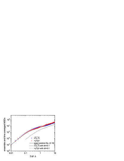
Figure 1: (Color online) The mean squared displacements (MSD) for FLE motion in free space. The ensemble averaged and time averaged MSDs, $\langle y^{2}(t)\rangle$ and $\overline{\delta^{2}(\Delta,T)}$, obtained from simulation are compared with the exact solution $2t^{2}E_{5/4,3}[-10\Gamma(5/4-1)t^{5/4}]$ given by Eq. (21). The ensemble averaged value was obtained from 200 simulated trajectories. In the simulation, we chose the Hurst exponent $\overline{H}=5/8$, time increment $dh=0.01$, particle mass $m=1$, initial velocity $v_{0}=1$, initial position $y_{0}=0$, friction coefficient $\overline{\gamma}=10$, and $k_{B}T=1$.

To show the reliability of our simulation, we compare the simulation result with the well-known solution for free space motion. In Fig. 1, we simulate the subdiffusion case with the parameters values, $\overline{H}=5/8$, $m=1$, $v_{0}=1$, $y_{0}=0$, $\overline{\gamma}=10$, $k_{B}T=1$, and $dh=0.01$. From 200 simulated trajectories, we obtain the ensemble averaged and time averaged mean squared displacements, $\langle y^{2}(t)\rangle$ and $\overline{\delta^{2}(\Delta,T)}$, and compare them with the exact solution Eq. (21). Note that $\langle y^{2}(t)\rangle$ should be identical to $\overline{\delta^{2}(\Delta,T)}$, Eq. (39), with $t$ regarded as the lag time $\Delta$ due to the ergodicity of the FLE motion in free space deng . The deviation from the exact solution is markedly reduced with decreasing time increment $dh$. With our chosen value $dh=0.01$ the mean squared displacements obtained from simulation appear to be in good agreement with the theory.

IV Fractional Brownian Motion in confined space

We now turn to the investigation of the behavior of FBM under confinement, analyzing the mean squared displacement and potential ergodicity breaking. We then define the displacement correlation function, and finally study the influence of dimensionality.

IV.1 Mean squared displacement

For FBM in free space $\langle x^{H}(t)^{2}\rangle$ can be estimated by the time averaged mean squared displacement Eq. (2) via the exact relation deng

$$\left<\overline{\delta^{2}(\Delta,T)}\right>=2K_{H}\Delta^{2H}.$$ (28)

Here $\langle\cdot\rangle$ denotes the ensemble average. In contrast to CTRW subdiffusion, in FBM this quantity is ergodic. However, as mentioned above, the approach to ergodicity is algebraically slow, and we want to explore here whether boundary conditions have an impact on the ergodic behavior. Let us now analyze the behavior in a box of size $2L$.

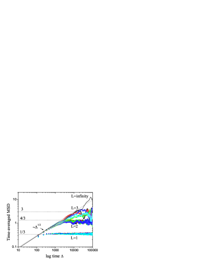
Figure 2: (Color online) Time-averaged mean squared displacement (MSD) versus the lag time $\Delta$ for given values of $L$. The drawn line has slope $1/2$, corresponding to the expected short lag time behavior for the used value $H=1/4$ of the Hurst exponent. For $L=1$, 2, and 3, five different trajectories each are drawn to be able to see whether the trajectories scatter. The simulation time is $T=2^{17}\approx 1.3\cdot 10^{5}$.

In Fig. 2 we show typical curves for the time averaged mean squared displacement for Hurst exponent $H=1/4$ and three different interval lengths $L$. Regardless of the size of $L$, the confined environment does not affect the power law with exponent $2H$ for short lag times. Moreover at long lag times we observe saturation of the curves to a value that depends on $L$. This behavior is distinct from that of the CTRW case where $\left<\overline{\delta^{2}(\Delta,T)}\right>$ shows a power law with slope $1-\alpha$ stas ; thomas .

One can estimate the saturated value as a function of $L$. For long $\Delta$ and measurement time $T$, the probability $p(x)$ to find the particle located at $x$ is independent of $x$ due to the equilibration between the reflecting walls, and thus $\int_{-L}^{L}x^{2}p(x)dx=L^{2}/3$. The dotted lines in Fig. 2 represent these values.

We observe that the scatter between different single trajectories becomes more pronounced when the interval length is increased. In fact the scatter is negligible for $L=1$ while it is quite appreciable for $L=3$, even though the slope of all curves at finite $L$ converges to a horizontal slope, with an amplitude close to the predicted value $L^{2}/3$. We also note that the scatter depends on the total measurement time $T$. For given $L$ it tends to be reduced as we increase $T$. This effect will be discussed quantitatively in detail using the ergodicity breaking parameter.

IV.2 Ergodicity breaking parameter

In contrast to CTRW subdiffusion, FBM in free space is known to be ergodic deng . The time averaged mean squared displacement traces displayed in Fig. 2 exhibit no extreme scatter as known from the CTRW case. This implies that ergodicity is indeed preserved for confined FBM. We quantify this statement more precisely in terms of the ergodicity breaking parameter YHe

$$E_{B}(\Delta,T)=\frac{\left<\left(\overline{\delta^{2}(\Delta,T)}\right)^{2}\right>-\left<\overline{\delta^{2}(\Delta,T)}\right>^{2}}{\left<\overline{\delta^{2}(\Delta,T)}\right>^{2}},$$ (29)

where $\lim_{T\rightarrow\infty}E_{B}(T)=0$ is expected for ergodic systems. For the case of free FBM, Deng and Barkai analytically derived that $E_{B}$ decays to zero as

$$E_{B}(\Delta,T)\sim\left\{\begin{array}[]{ll}\displaystyle\frac{\Delta}{T}&\mbox{for}~{}0<H<\frac{3}{4},\\[11.38092pt] \displaystyle\frac{\Delta}{T}\log T&\mbox{for}~{}H=\frac{3}{4},\\[11.38092pt] \displaystyle\left(\frac{\Delta}{T}\right)^{4-4H}&\mbox{for}~{}\frac{3}{4}<H<1,\end{array}\right.$$ (33)

for long measurement time $T$ deng .

We numerically investigate the boundary effects on the ergodicity breaking parameter. First, in Fig. 3 we evaluate $E_{B}$ as function of the lag time $\Delta$ from 200 FBM simulations for each given $L$. The dotted line represents the expected free space behavior $E_{B}\sim\Delta$, which is nicely fulfilled by the data at shorter times and sufficiently large $L$. At longer times or small $L$ the results show that $E_{B}$ behaves very differently when confinement effects are present. The plateau in $E_{B}$ is related to the saturation of the curves for the mean squared displacement, Fig. 2. As the motion is restricted by the walls roughly above a crossover lag time $\Delta_{cr}=(L^{2}/2K_{H})^{1/2H}$, the ergodicity breaking parameter $E_{B}$ levels off at $\Delta\gtrsim\Delta_{cr}$. The sharp increase at the end of the curve is due to the singularity when the lag time reaches the size of the overall measurement time $T$, which would disappear in the infinite measurement time.

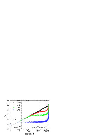
Figure 3: (Color online) Ergodicity breaking parameter $E_{B}$ versus lag time $\Delta$ for $L=1$, 3, 5, and 10 (from bottom to top) with Hurst exponent $H=1/4$. The overall measurement time is $T=2^{14}\approx 1.6\cdot 10^{4}$. The dotted line with slope 1 represents the theoretical expectation $E_{B}\simeq\Delta$ in free space. For each $L$ the curve was obtained from 200 single trajectories. The vertical lines show the crossover lag time $\Delta_{cr}=(L^{2}/2K_{H})^{1/2H}$ for $L=1,~{}3$, and 5.

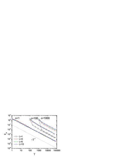
Figure 4: (Color online) Ergodicity breaking parameter $E_{B}$ versus overall measurement time $T$ at given lag time $\Delta=1$, 100, and 1000. The dotted line depicts a power law with slope -1, representing the analytic behavior $E_{B}\simeq T^{-1}$ in free space. For each $\Delta$, the $E_{B}$ curves are drawn for different interval lengths $L=1$, 3, 5, and 10. Each curve was obtained from 200 single trajectories, and the Hurst exponent was $H=1/4$.

In Fig. 4 we show $E_{B}$ for given $\Delta$ as function of the measurement time $T$ for the same choice of interval lengths, $L=1,3,5$, and 10. For short lag times $\Delta$, all $E_{B}$ curves coincide and decay as $T^{-1}$, in complete analogy to the free space motion (dotted line). In the case of longer $\Delta$ the general trend is that $E_{B}$ decays like $T^{-1}$, unaltered with respect to the free case. However, there is a sudden decrease in $E_{B}$ for the smallest interval size, for $L=1$. One can understand this behavior by observing the $E_{B}$ curve for $L=1$ in Fig. 3; as the fluctuations of the mean squared displacement are strongly suppressed due to the tight confinement in this case, $E_{B}$ has almost no dependence on $\Delta$ for $\Delta_{cr}\lesssim\Delta\lesssim T$ and the saturated value is quite small compared to those for other cases. Therefore, the curves for $L=1$ appear disconnected from the other curves. Corresponding to the approximate independence of the $L=1$ curve for $\Delta\gtrsim 10$ in Fig. 3, we observe in Fig. 4 that at longer times $T$ the $L=1$ curves approach each other. Only at $T\approx\Delta$ these curves separate, as then $\overline{\delta_{i}^{2}(T,T)}=[x^{H}_{i}(t+T)-x^{H}_{i}(t)]^{2}$, and $E_{B}$ is evaluated with the same small number of squared displacement data. Note that the splitting of the $E_{B}$ curve can be also observed for larger $L$ at $\Delta$s larger than $\Delta_{cr}$ under longer total measurement time $T$ as other $E_{B}$ curves also have corresponding constant saturation values for $\Delta\gtrsim\Delta_{cr}(=(L^{2}/2K_{H})^{1/2H})$ which increases with the size $L$.

IV.3 Displacement correlation function

As explained for the stochastic properties of FBM in Sec. II, the position autocorrelation $\langle x^{H}(t_{1})x^{H}(t_{2})\rangle$ explicitly depends on $t_{1}$ and $t_{2}$ as well as their difference, $|t_{1}-t_{2}|$. It is therefore not an efficient quantity to estimate directly from experimental or simulations data. However, the correlation function of the displacements

$$\delta x^{H}(t,\Delta)=x^{H}(t+\Delta)-x^{H}(t)$$ (34)

depends only on the time interval $\Delta$ of the displacement,

$$\langle\delta x^{H}(t,\Delta)\delta x^{H}(t-\Delta,\Delta)\rangle=K_{H}(2^{2H}-2)\Delta^{2H}$$ (35)

for free FBM. This relation is derived in App. A. This quantity is anticorrelated for $0<H<1/2$ (subdiffusive motion), uncorrelated for $H=1/2$ (normal Brownian motion), and positively correlated for $1/2<H<1$ (superdiffusion). As Eq. (35) does not depend on the measurement time $T$ the value of the ensemble averaged value is identical to the corresponding time average.

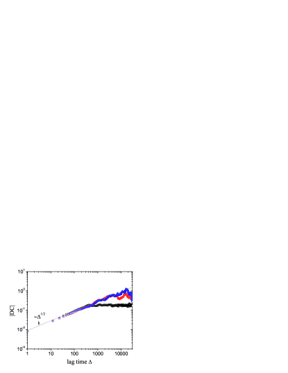
Figure 5: (Color online) Absolute value of the displacement correlation (DC) versus lag time $\Delta$ for $L=1$, 2, and 3 (from bottom to top) with a slope proportional to $\Delta^{2H}$ (dotted line). Total measurement time is $T=2^{17}\approx 1.3\cdot 10^{5}$, and the Hurst exponent is $H=1/4$. Each curve was obtained via time averaging from a single particle trajectory.

We present the time averaged displacement correlation for confined subdiffusive motion ($H=1/4$) in Fig. 5. Because of the negativity of expression (35) the absolute value of the displacement correlation is drawn in the log-log representation. At short lag times the slope of the correlation functions is proportional to $2H$ as expected from Eq. (35). However, at long lag times, we interestingly observe fluctuations of the correlations around a constant value, reflecting the confinement of the motion.

IV.4 Dimensionality

To mimic the anomalous diffusion of particles inside biological cells, we also simulate two- and three-dimensional FBM based on Eq. (9) in the presence of reflecting walls. In free space, the ensemble average of the time averaged mean squared displacement is simply given by

$$\left<\overline{\delta^{2}(\Delta,T)}\right> = \frac{1}{T-\Delta}\int_{0}^{T-\Delta}\left<[{\mathbf{x}}^{H}(t+\Delta)-{\mathbf{x}}^{H}(t)]^{2}\right>dt,$$ (36)

$$= 2dK_{H}\Delta^{2H},$$

i.e., it is additive as for the ensemble average. This behavior is indeed observed in Fig. 6 where five different mean squared displacement curves are drawn for $L=1$ in 1D, 2D, and 3D, respectively. Only the height of the curves are affected by the dimensionality. There is no noticeable difference in the scatter of the curves.

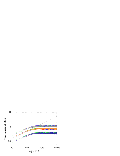
Figure 6: (Color online) Time-averaged mean squared displacement (MSD) curves versus lag time $\Delta$ for $L=1$ in 1D, 2D, and 3D space (from bottom to top), with a slope $\Delta^{2H}$ (dotted line). For each dimension, 5 trajectories were drawn with total measurement time $T=2^{17}$ and $H=1/4$.

We further investigate the effects of dimensionality on the scatter of the mean squared displacement curves, as possibly the strong scatter observed in experiments golding ; lene ; elbaum may also occur for FBM in higher dimensions. To see the effect of dimensionality on the ergodicity behavior we measure $E_{B}$ versus lag time for one-, two-, and three-dimensional embedding dimension for the same values of $L$ and $H$. Interestingly, the result shows that $E_{B}$ tends to decrease with increasing dimensionality $d$, meaning that for FBM big scatter is not caused by higher dimensions in presence of reflecting walls. In fact, from Eqs. (29) and (36), we can analytically derive the relation

$$E_{B}(d)=\frac{E_{B}(d=1)}{d},$$ (37)

which still holds in the case of confined motion (see appendix B for the derivation). This relation is numerically confirmed in Fig. 7 where three $E_{B}$ curves collapse upon rescaling by $dE_{B}(d)$. According to this relation, we expect that ergodic behavior obtained in one-dimensional confined motion (Figs. 3 and 4) will also be present in multiple dimensions with a factor of $1/d$.

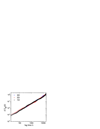
Figure 7: (Color online) Rescaled ergodicity breaking parameter $dE_{B}$ versus lag time $\Delta$ for interval size $L=5$ for 1D, 2D, and 3D space (from top to bottom), with Hurst exponent $H=1/4$ and measurement time $T=2^{14}$. $E_{B}$ was evaluated from 200 trajectories with different initial positions.

V Fractional Langevin equation motion in confined space

In this section we analyze FLE motion under confinement. Due to the different physical basis compared to FBM, in particular, the occurrence of inertia, we observe interesting variations on the properties studied in the previous section.

V.1 Mean squared displacement

Using the correlation function pottier

$$\langle y(t_{1})y(t_{2})\rangle = \frac{k_{B}T}{m}[t_{1}^{2}E_{2\overline{H},3}(-\gamma t_{1}^{2\overline{H}})+t_{2}^{2}E_{2\overline{H},3}(-\gamma t_{2}^{2\overline{H}})$$ (38)

$$-(t_{2}-t_{1})^{2}E_{2\overline{H},3}(-\gamma|t_{2}-t_{1}|^{2\overline{H}})],$$

one can show analytically that, similarly to the FBM, the ensemble averaged second moment $\langle y^{2}(t)\rangle$ is identical to its time averaged analog $\left<\overline{\delta^{2}(\Delta)}\right>$, for all $\Delta$ in free space, namely

$$\left<\overline{\delta^{2}(\Delta,T)}\right>=2\frac{k_{B}T}{m}\Delta^{2}E_{2\overline{H},3}(-\gamma\Delta^{2\overline{H}}).$$ (39)

Thus, the time averaged mean squared displacement turns over from a ballistic motion

$$\left<\overline{\delta^{2}(\Delta,T)}\right>\simeq\Delta^{2}$$ (40)

at short lag time to the subdiffusive behavior

$$\left<\overline{\delta^{2}(\Delta,T)}\right>\simeq\Delta^{2-2\overline{H}}$$ (41)

at long lag times, in free space.

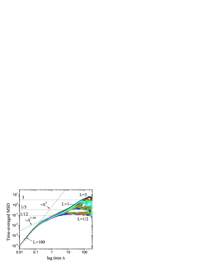
Figure 8: (Color online) Time-averaged mean squared displacement (MSD) versus lag time $\Delta$. The two dashed lines represent the two asymptotic scaling behaviors $\left<\overline{\delta^{2}(\Delta,T)}\right>\simeq\Delta^{2}$ and $\left<\overline{\delta^{2}(\Delta,T)}\right>\simeq\Delta^{2-2\overline{H}}$. For each given $L=1/2$, 1, and 3, five different trajectories are drawn to visualize the scatter. As a reference curve for motion in free space, the curve for $L=100$ (line) is drawn. In the simulation, we chose the Hurst exponent $\overline{H}=5/8$ [NB: for the FLE this means subdiffusion], time increment $dh=0.01$, particle mass $m=1$, initial velocity $v_{0}=1$, initial position $y_{0}=0$, friction coefficient $\overline{\gamma}=10$, and $k_{B}T=1$.

We numerically study how this scaling behavior is affected by the confinement. Figure 8 shows typical curves for the time averaged mean squared displacement, for interval sizes $L=1/2$, 1, 3, and 100 (regarded as free space motion) with identical initial conditions and Hurst exponent $\overline{H}=5/8$. The results are summarized as follows: (1) We observe both scaling behaviors, $\left<\overline{\delta^{2}(\Delta,T)}\right>\simeq\Delta^{2}$ turning over to $\simeq\Delta^{2-2\overline{H}}$, for confined FLE motions. (2) For narrow intervals, the curves eventually reach the saturation plateau within the chosen total measurement time $T$. The saturation values are approximately $L^{2}/3$. For interval size $L=1/2$, the saturated value is noticeably larger than $L^{2}/3$, which appears to be caused by multiple reflection events on the walls. The same behavior is observed in the FBM case when considering a large value of $H\geq 1/2$, or very narrow intervals for the given $H=1/4$. (3) As in the case of FBM, the scatter becomes pronounced as the interval length increases.

V.2 Ergodicity breaking parameter

From a simple argument and simulations it was shown in Ref. deng that the FLE and FBM mean squared displacements are asymptotically equal, $\left<\overline{\delta^{2}(y)}\right>\sim\left<\overline{\delta^{2}(x^{H})}\right>$, similarly for the ergodicity breaking parameter, $E_{B}(y)\sim E_{B}(x^{H})$. Here the asymptotic equivalence is valid at long measurement times $T$, and the derivation holds for motion in free space. From 200 trajectories of the mean squared displacement we measure the ergodicity breaking parameter $E_{B}$ as function of lag time $\Delta$ for interval lengths $L=1/2$, 1, 3, and 100 in Fig. 9. The behavior is similar to the corresponding curves for FBM, displayed in Fig. 3: $E_{B}$ significantly deviates from the reference curve for free space motion (i.e., the longer $\Delta$ behavior for $L=100$ and the drawn power law $\simeq\Delta$), due to the confinement effect. $E_{B}$ tends to decrease with smaller $L$ for the same value of $\Delta$. However, the plateau at short lag times that is still observed for $L=100$ (regarded as free space motion), is due to the initial ballistic motion of FLE. In that regime the initially directed motion renders the random noise effect negligible.

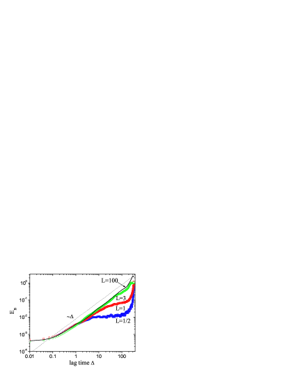
Figure 9: (Color online) Ergodicity breaking parameter $E_{B}$ versus lag time $\Delta$ for interval sizes $L=1/2$, 1, 3, and 100. The straight line corresponds to the free space behavior $E_{B}\simeq\Delta$. Each curve was obtained from 200 single trajectories, with the same parameter values used in Fig. 8.

V.3 Displacement correlation function

Using the correlation function $\langle y(t_{1})y(t_{2})\rangle$, we analytically obtain the displacement correlation function in free space in the form (refer to App. A for the derivation)

$$\langle\delta y(t,\Delta)\delta y(t-\Delta,\Delta)\rangle = 4\frac{k_{B}T}{m}\Delta^{2}E_{2\overline{H},3}[-\gamma(2\Delta)^{2\overline{H}}]$$ (42)

$$-2\frac{k_{B}T}{m}\Delta^{2}E_{2\overline{H},3}[-\gamma\Delta^{2\overline{H}}],$$

so that we observe the following asymptotic behavior

$$\langle\delta y(t,\Delta)\delta y(t-\Delta,\Delta)\rangle$$ (45)

$$\sim\left\{\begin{array}[]{ll}\displaystyle\frac{2k_{B}T}{m\Gamma(3)}\Delta^{2}&\mbox{for }\Delta\rightarrow 0,\\[11.38092pt] \displaystyle\frac{(2^{2-2H}-2)k_{B}T}{m\gamma\Gamma(3-2\overline{H})}\Delta^{2-2\overline{H}}&\mbox{for }\Delta\rightarrow\infty,\end{array}\right.$$

where $\delta y(t,\Delta)=y(t+\Delta)-y(t)$. Above expression shows that the displacement correlation has two distinct scaling behaviors. At short lag times, it grows like $\Delta^{2}$ and is positive, due to the ballistic motion. At long lag times, it is negative in the domain $1/2<\overline{H}<1$, exhibiting the same subdiffusive behavior as observed for FBM [cf. Eq. (35)] when we replace $H\rightarrow 2-2\overline{H}$. Note that to bridge these two scaling behaviors the displacement correlation passes the zero axis at $\Delta=\Delta_{c}$ that satisfies $2E_{2\overline{H},3}\left[-\gamma(2\Delta_{c})^{2\overline{H}}\right]=E_{2\overline{H},3}\left[-\gamma\Delta_{c}^{2\overline{H}}\right]$ in free space. For small $\gamma$, we find approximately

$$\Delta_{c}\approx\left(\frac{\Gamma(2\overline{H}+3)}{2\Gamma(2\overline{H}-1)(2^{2\overline{H}+1}-1)}\frac{m}{\overline{\gamma}}\right)^{1/2\overline{H}},$$ (46)

such that it becomes exactly the momentum relaxation time $m/\overline{\gamma}$ for normal Brownian motion ($\overline{H}=1/2$). In the limit $\overline{H}\rightarrow 1$, $\Delta_{c}$ goes to infinity to satisfy the equality $2E_{2\overline{H},3}\left[-\gamma(2\Delta_{c})^{2\overline{H}}\right]=E_{2\overline{H},3}\left[-\gamma\Delta_{c}^{2\overline{H}}\right]$. Thus, $\Delta_{c}$ can be interpreted as the typical timescale for the persistence of the ballistic motion.

Figure 10 shows (a) the displacement correlation versus lag time $\Delta$, and (b) the absolute value of the displacement correlation as function of $\Delta$, for $L=1/2$, 1, 3, and 100. The scaling properties derived in Eq. (45) are indeed observed. At short lag times all curves are positive and scale like $\sim\Delta^{2}$, before decreasing to zero. In the long lag time regime the displacement correlation becomes negative and the predicted scaling behavior $\simeq\Delta^{2-2\overline{H}}$ is observed. For small intervals ($L=1/2$ and 1), it is saturated due to the confinement effect as seen in the case of FBM.

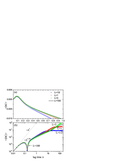
Figure 10: (Color online) (a) Displacement correlation (DC) versus lag time $\Delta$ for $L=1/2$, 1, 3, and 100 (from bottom to top). (b) Absolute value of the displacement correlation as a function of $\Delta$ for the given values of $L$. The two slopes correspond to the limiting behavior $\Delta^{2}$ and $\Delta^{2-2\overline{H}}$. In (a) and (b), the ensemble averaged curves were obtained from 200 different time averaged displacement correlation curves. Same parameter values as in Fig. 8.

V.4 Dimensionality

In the case when the memory tensor is diagonalized, each coordinate motion is independent and FLE motion exhibits qualitatively the same behavior as shown in the case of FBM with increasing dimensionality. From the mean squared displacement curves, the same scaling behavior is expected with more elevated amplitude for higher dimensionality. In fact, when each coordinate motion is decoupled, a $d$-dimensional motion effectively increases the number of single trajectories $d$ times compared to the one-dimensional case. Therefore, the scatter in the mean square displacement curves decreases with increasing dimensionality and the ergodicity breaking parameter $E_{B}$ is expected to follow the relation Eq. (37).

VI Conclusion

Motivated by recent single particle tracking experiments in biological cells, in which confinement due to the rather small cell size becomes relevant, we studied FBM and FLE motions in confined space. In particular we analyzed the effects of confinement and dimensionality on the stochastic and ergodic properties of the two processes. Interestingly for both stochastic models, the confinement tends to decrease the value of the ergodicity breaking parameter $E_{B}$ compared to that in free space. The same trend is observed for increasing dimensionality. Correspondingly the scatter of time averaged quantities between individual trajectories is quite small, apart from regimes when the lag time $\Delta$ becomes close to the overall measurement time $T$ and the sampling statistics for the corresponding time average become poor. The relaxation of the ergodicity breaking parameter as function of measurement time is quite similar to previous results in free space. We conclude that neither confinement nor dimensionality effects lead to the appearance of significant ergodicity breaking or scatter between single trajectories.

The displacement correlation function introduced here is a useful quantity that can be easily obtained from single particle trajectories. It can be used as a tool to discriminate one stochastic model from another. For subdiffusive motion governed by FBM and FLE motion, the displacement correlation should be negative and saturate in the long measurement time limit due to the confinement. Notably, the negative decrease ($\sim-\Delta^{\alpha}$) with lag time $\Delta$ and anomalous diffusion exponent $\alpha$ is an intrinsic property of FBM and FLE displacement correlations which is clearly distinguished from that of CTRW subdiffusion. In the latter case, the subdiffusive motion occurs due to the long waiting time distribution between successive jumps and there is no spatial correlation between them, so that displacement correlation only fluctuates around zero with time. FLE motion can be distinguished from FBM motion since the displacement correlation has a positive value at short times due to the ballistic motion in the FLE model.

Appendix A Derivation of the displacement correlation function

In this appendix we derive analytical expressions for the displacement correlations, Eqs. (35) and (42). For a stochastic variable $x$, we define

$$\delta x(t,\Delta)=x(t+\Delta)-x(t).$$ (47)

The displacement correlation is then given by

$$\langle\delta x(t,\Delta)\delta x(t-\Delta,\Delta)\rangle=$$

$$\hskip 22.76228pt\langle x(t+2\Delta)x(t+\Delta)\rangle-\langle x(t+2\Delta)x(t)\rangle$$

$$\hskip 22.76228pt-\langle x(t+\Delta)^{2}\rangle+\langle x(t+\Delta)x(t)\rangle.$$ (48)

We now calculate this expression for FBM and FLE motions.

A.1 FBM

For FBM ($x(t)=x^{H}(t)$), we use the expression

$$\langle x(t_{1})x(t_{2})\rangle=K_{H}(t_{1}^{2H}+t_{2}^{2H}-|t_{2}-t_{1}|^{2H})$$ (49)

for the autocorrelation. With this we readily obtain the result

$$\langle\delta x(t,\Delta)\delta x(t-\Delta,\Delta)\rangle=K_{H}(2^{2H}-2)\Delta^{2H}.$$ (50)

A.2 FLE

For FLE ($x(t)=y(t)$), we use the correlation function pottier

$$\langle x(t_{1})x(t_{2})\rangle = \frac{k_{B}T}{m}[t_{1}^{2}E_{2\overline{H},3}(-\gamma t_{1}^{2\overline{H}})+t_{2}^{2}E_{2\overline{H},3}(-\gamma t_{2}^{2\overline{H}})$$ (51)

$$-(t_{2}-t_{1})^{2}E_{2\overline{H},3}(-\gamma|t_{2}-t_{1}|^{2\overline{H}})].$$

The displacement correlation is then obtained as

$$\langle\delta x(t,\Delta)\delta x(t-\Delta,\Delta)\rangle$$

$$\hskip 34.14322pt=\frac{4k_{B}T}{m}\Delta^{2}E_{2\overline{H},3}\left[-\gamma(2\Delta)^{2\overline{H}}\right]$$

$$\hskip 34.14322pt-\frac{2k_{B}T}{m}\Delta^{2}E_{2\overline{H},3}[-\gamma\Delta^{2\overline{H}}].$$ (52)

Expanding the generalized Mittag-Leffler function $E_{2\overline{H},3}(x)\approx 1/\Gamma(3)+x/\Gamma(2\overline{H}+3)+\cdots$ for $x\ll 1$ the displacement correlation is approximated as

$$\langle\delta x(t,\Delta)\delta x(t-\Delta,\Delta)\rangle\sim\frac{2}{\Gamma(3)}\frac{k_{B}T}{m}\Delta^{2}$$ (53)

at short lag times. With the expansion $E_{2\overline{H},3}(-x)\approx 1/x\Gamma(3-2\overline{H})$ for $x\gg 1$ the long lag time behavior of the displacement correlation is obtained as

$$\langle\delta x(t,\Delta)\delta x(t-\Delta,\Delta)\rangle\sim\frac{2^{2-2\overline{H}}-2}{\gamma\Gamma(3-2\overline{H})}\frac{k_{B}T}{m}\Delta^{2-2\overline{H}}.$$ (54)

Note that the prefactor $(2^{2-2\overline{H}}-2)/\Gamma(3-2\overline{H})$ is zero for $\overline{H}=1/2$ and then becomes increasingly negative, saturating at the value 1 for $\overline{H}=1$.

Appendix B Derivation of Equation (37)

From the definition of the time averaged mean squared displacement, Eq. (36), we expand $\left<\left(\overline{\delta^{2}(\Delta,T)}\right)^{2}\right>$ in the form

$$\left<\left(\overline{\delta^{2}(\Delta,T)}\right)^{2}\right>=\frac{1}{(T-\Delta)^{2}}\int_{0}^{T-\Delta}\int_{0}^{T-\Delta} \Big{\{} \sum_{i=1}^{d}\langle[x_{i}^{H}(t_{1}+\Delta)-x_{i}^{H}(t_{1})]^{2}[x_{i}^{H}(t_{2}+\Delta)-x_{i}^{H}(t_{2})]^{2}\rangle$$ (55)

$$+\sum_{i\neq j}\langle[x_{i}^{H}(t_{1}+\Delta)-x_{i}^{H}(t_{1})]^{2}\rangle\langle[x_{j}^{H}(t_{2}+\Delta)-x_{j}^{H}(t_{2})]^{2}\rangle\Big{\}}dt_{1}dt_{2}.$$

Using the Isserlis theorem for Gaussian process with zero mean coffey :

$$\langle x(t_{1})x(t_{2})x(t_{3})x(t_{4})\rangle=\langle x(t_{1})x(t_{2})\rangle\langle x(t_{3})x(t_{4})\rangle+\langle x(t_{1})x(t_{3})\rangle\langle x(t_{2})x(t_{4})\rangle+\langle x(t_{1})x(t_{4})\rangle\langle x(t_{2})x(t_{3})\rangle,$$ (56)

the first term in the braces in Eq. (55) can be rewritten as

$$\sum_{i=1}^{d}\langle[x_{i}^{H}(t_{1}+\Delta)-x_{i}^{H}(t_{1})]^{2}[x_{i}^{H}(t_{2}+\Delta)-x_{i}^{H}(t_{2})]^{2}\rangle=\sum_{i=1}^{d}\langle[x_{i}^{H}(t_{1}+\Delta)-x_{i}^{H}(t_{1})]^{2}\rangle\langle[x_{i}^{H}(t_{2}+\Delta)-x_{i}^{H}(t_{2})]^{2}\rangle$$

$$\hskip 193.47882pt+2\sum_{i=1}^{d}\langle[x_{i}^{H}(t_{1}+\Delta)-x_{i}^{H}(t_{1})][x_{i}^{H}(t_{2}+\Delta)-x_{i}^{H}(t_{2})]\rangle^{2}.$$ (57)

In this expression, we note that the sum of the second term in Eq. (55) and the first term in Eq. (57) yields $\left<\overline{\delta^{2}(\Delta,T)}\right>^{2}$:

$$\left<\overline{\delta^{2}(\Delta,T)}\right>^{2} = \frac{d^{2}}{(T-\Delta)^{2}}\int_{0}^{T-\Delta}\int_{0}^{T-\Delta}\langle[x^{H}(t_{1}+\Delta)-x^{H}(t_{1})]^{2}\rangle\langle[x^{H}(t_{2}+\Delta)-x^{H}(t_{2})]^{2}\rangle dt_{1}dt_{2}$$ (58)

$$= d^{2}\langle\overline{\delta^{2}}\rangle_{1D}^{2},$$

where we used the property

$$\sum_{i,j}\langle[x_{i}^{H}(t_{1}+\Delta)-x_{i}^{H}(t_{1})]^{2}\rangle\langle[x_{j}^{H}(t_{2}+\Delta)-x_{j}^{H}(t_{2})]^{2}\rangle=d^{2}\langle[x^{H}(t_{1}+\Delta)-x^{H}(t_{1})]^{2}\rangle\langle[x^{H}(t_{2}+\Delta)-x^{H}(t_{2})]^{2}\rangle$$ (59)

due to the independence of the motion in each coordinate direction. We also note that the expression $\left<\left(\overline{\delta^{2}(\Delta,T)}\right)^{2}\right>-\left<\overline{\delta^{2}(\Delta,T)}\right>^{2}$ simplifies to

$$\left<(\overline{\delta^{2}(\Delta,T})^{2}\right>-\langle\overline{\delta^{2}}\rangle^{2} = \frac{2}{(T-\Delta)^{2}}\sum_{i=1}^{d}\int_{0}^{T-\Delta}\int_{0}^{T-\Delta}\langle[x_{i}^{H}(t_{1}+\Delta)-x_{i}^{H}(t_{1})]\times[x_{i}^{H}(t_{2}+\Delta)-x_{i}^{H}(t_{2})]\rangle^{2}dt_{1}dt_{2}$$ (60)

$$= d[\langle(\overline{\delta^{2}})^{2}\rangle_{1D}-\langle\overline{\delta^{2}}\rangle_{1D}^{2}].$$

From Eqs. (58) and (60), the ergodicity breaking parameter follows the general relation

$$E_{B}(d)=\frac{\left<\left(\overline{\delta^{2}(\Delta,T)}\right)^{2}\right>-\left<\overline{\delta^{2}(\Delta,T)}\right>^{2}}{\left<\overline{\delta^{2}(\Delta,T)}\right>^{2}}=\frac{E_{B}(d=1)}{d}.$$ (61)

References

- (1) R. Metzler and J. Klafter, Phys. Rep. 339 1 (2000); J. Phys. A 37, R161 (2004).
- (2) H. Scher and E. W. Montroll, Phys. Rev. B 12, 2455 (1975).
- (3) J. W. Kirchner, X. Feng, and C. Neal, Nature 403, 524 (2000); H. Scher, G. Margolin, R. Metzler, J. Klafter, and B. Berkowitz, Geophys. Res. Lett. 29, 1061 (2002).
- (4) F. Mainardi, M. Raberto, R. Gorenflo, and E. Scalas, Physica A 287, 468 (2000).
- (5) I. Y. Wong, M. L. Gardel, D. R. Reichman, E. R. Weeks, M. T. Valentine, A. R. Bausch, and D. A. Weitz, Phys. Rev. Lett. 92, 178101 (2004).
- (6) E. Fischer, R. Kimmich, and N. Fatkullin, J. Chem. Phys. 104, 9174 (1996).
- (7) E. R. Weeks, J. C. Crocker, A. C. Levitt, A. Schofield, and D. A. Weitz, Science 287, 627 (2000).
- (8) I. Golding and E. C. Cox, Phys. Rev. Lett. 96, 098102 (2006).
- (9) I. M. Tolić-Nørrelykke, E. L. Munteanu, G. Thon, L. Oddershede, and K. Berg-Sørensen, Phys. Rev. Lett. 93, 078102 (2004).
- (10) A. Caspi, R. Granek, and M. Elbaum, Phys. Rev. Lett. 85, 5655 (2000); Phys. Rev. E. 66, 011916 (2002).
- (11) G. Seisenberger, M. U. Ried, T. Endreß, H. Büning, M. Hallek, and C. Bräuchle, Science 294, 1929 (2001).
- (12) I. Bronstein, Y. Israel, E. Kepten, S. Mai, Y. Shav-Tal, E. Barkai, and Y. Garini, Phys. Rev. Lett. 103, 018102 (2009).
- (13) M. Weiss, M. Elsner, F. Kartberg, and T. Nilsson, Biophys. J. 87, 3518 (2004); M. Weiss, H. Hashimoto, and T. Nilsson, ibid. 84, 4043 (2003). Note: HeLa cells belong to an immortal cell line derived from cancer cells originally taken from Henrietta Lacks in 1951.
- (14) V. Tejedor and R. Metzler (unpublished).
- (15) S. Havlin and D. ben-Avraham, Adv. Physics 36, 695 (1987).
- (16) A. Klemm, R. Metzler, and R. Kimmich, Phys. Rev. E 65, 021112 (2002).
- (17) G. M. Molchan, Commun. Math. Phys. 205, 97 (1999).
- (18) I. Goychuk and P. Hänggi, Phys. Rev. Lett. 99, 200601 (2007).
- (19) S. Chaudhury and B. J. Cherayil, J. Chem. Phys. 125, 024906 (2006); S. Chaudhury, D. Chatterjee, and B. J. Cherayil, ibid. 129, 075104 (2008).
- (20) O. Yu. Slyusarenko, V. Yu. Gonchar, A. V. Chechkin, I. M. Sokolov, and R. Metzler (unpublished).
- (21) I. Goychuk, Phys. Rev. E 80, 046125 (2009).
- (22) S. Burov and E. Barkai, Phys. Rev. Lett. 100, 070601 (2008).
- (23) Y. He, S. Burov, R. Metzler, and E. Barkai, Phys. Rev. Lett. 101, 058101 (2008); A. Lubelski, I. M. Sokolov, and J. Klafter, ibid. 100, 250602 (2008).
- (24) R. Metzler, V. Tejedor, J.-H. Jeon, Y. He, W. Deng, S. Burov, and E. Barkai, Acta Phys. Polon. B 40, 1315 (2009).
- (25) W. Deng and E. Barkai, Phys. Rev. E 79, 011112 (2009).
- (26) J.-D. Bao, P. Hänggi, and Y.-Z. Zhuo, Phys. Rev. E. 72, 061107 (2005).
- (27) S. Burov, R. Metzler, and E. Barkai (unpublished).
- (28) T. Neusius, I. M. Sokolov, and J. C. Smith, Phy. Rev. E 80, 011109 (2009).
- (29) A. N. Kolmogorov, Doklady Akademii Nauk SSSR (N.S.) 26, 115 (1940).
- (30) A. M. Yaglom, American Mathematical Society Translations Series 2 8, 87 (1958).
- (31) B. B. Mandelbrot, Comptes Rendus (Paris) 260, 3274 (1965).
- (32) B. B. Mandelbrot and J. W. van Ness, SIAM Rev. 10, 422 (1968).
- (33) H. E. Hurst, Trans. Am. Soc. Civ. Eng. 116, 770 (1951); H. E. Hurst, R. O. Black, and Y. M. Simaika, Long term storage: an experimental study (Constable, London, 1965).
- (34) I. Adelman, Amer. Econom. Rev. 60, 444 (1965); C. W. J. Granger, Econometrica 34, 150 (1966).
- (35) J. Szymanski and M. Weiss, Phys. Rev. Lett. 103, 038102 (2009).
- (36) V. Tejedor, O. Bénichou, R. Voituriez, R. Jungmann, F. Simmel, C. Selhuber, L. Oddershede, and R. Metzler (to appear in Biophs. J.).
- (37) F. Biagini, Y. Hu, B. Øksendal, and T. Zhang, Stochastic calculus for fractional Brownian motion and applications (Springer, Berlin, 2008).
- (38) A. Weron and M. Magdziarz, Euro. Phy. Lett. 86, 60010 (2009).
- (39) H. Qian, Process with Long-Range Correlations: Theory and Applications, Lecture Notes in Physics Vol. 621, edited by G. Rangarajan and M. Z. Ding (Springer, New York, 2003).
- (40) S. C. Kou and X. S. Xie, Phys. Rev. Lett. 93, 180603 (2004).
- (41) The autocorrelation function for becomes positive at due to the second term in Eq. (II.1) and has the property .
- (42) J. Feder, Fractals (Plenum Press, New York, 1988); B. B. Mandelbrot, The fractal geometry of nature (W. H. Freeman and Company, New York, 1977).
- (43) J. Unterberger, Ann. Prob. 37, 565 (2009).
- (44) H. Qian, G. M. Raymond, and J. B. Bassingthwaighte, J. Phys. A 31, L527 (1998).
- (45) K. Falconer, Fractal geometry: mathematical foundations and applications (Wiley, Chichester, UK, 1990).
- (46) P. Langevin, Comptes Rendus 146, 530 (1908).
- (47) N. G. van Kampen, Stochastic Processes in Physics and Chemistry (North-Holland, Amsterdam, 1981).
- (48) W. T. Coffey, Y. P. Kalmykov, and J. T. Waldron, The Langevin equation: with applications to stochastic problems in physics, chemistry and electrical engineering, second edition (World Scientific, Singapore, 2003).
- (49) R. Zwanzig, Nonequilibrium Statistical Mechanics (Oxford University Press, Oxford, UK, 2001).
- (50) R. Kubo in Tokyo lectures in theoretical physics, edited by R. Kubo (W. A. Benjamin, Inc., New York, NY, 1966).
- (51) B. J. Berne, J. P. Boon, and S. A. Rice, J. Chem. Phys. 45, 1086 (1966).
- (52) I. Podlubny, Fractional differential equations (Academic Press, New York, 1998).
- (53) A. Erdélyi, editor, Bateman Manuscript Project: Higher Transcendental Functions, Vol. III (McGraw-Hill Book Co., New York, NY, 1955).
- (54) E. Lutz, Phys. Rev. E. 64, 051106 (2001).
- (55) N. Pottier, Physica A 317, 371 (2003).
- (56) J. R. M. Hosking, Water Res. Res. 20 1898 (1984).
- (57) K. Diethelm, N. J. Ford, and A. D. Freed, Nonlinear Dynamics 29, 3 (2002).