The 3-dimensional cube is the only periodic,
connected cubic graph with perfect state transfer

Abstract

There is perfect state transfer between two vertices of a graph, if a single excitation can travel with fidelity one between the corresponding sites of a spin system modeled by the graph. When the excitation is back at the initial site, for all sites at the same time, the graph is said to be periodic. A graph is cubic if each of its vertices has a neighbourhood of size exactly three. We prove that the 3-dimensional cube is the only periodic, connected cubic graph with perfect state transfer. We conjecture that this is also the only connected cubic graph with perfect state transfer.

I Introduction

I.1 State transfer

Let $G=(V,E)$ be a graph with set of vertices $V(G)=\{1,2,...,n\}$ and set of edges $E(G)\subseteq V(G)\times V(G)-\{\{i,i\}:i\in V(G)\}$. The order of $G$ is the number of its vertices.

Let us consider a system of $n$ spin-$1/2$ quantum particles with unit $XY$ couplings. The space assigned to the entire system is $\left(\mathbb{C}^{2}\right)^{\otimes n}$. Each particle is attached to a vertex of $G$. The coupling between two particles is nonzero if and only if the particles are attached to adjacent vertices. The couplings are then specified by the adjacency matrix of the graph. The $ij$-th entry of the adjacency matrix of $G$ is $[A(G)]_{i,j}=1$ if $\{i,j\}\in E(G)$ and $[A(G)]_{ij}=0$ if $\{i,j\}\notin E(G)$.

We shall work with the XY model. Let $X_{i}$ and $Y_{i}$ be the Pauli operators acting on the $i$-th particle. The Hamiltonian governing the dynamics of the spin system can be written as $H_{XY}(G)=2^{-1}\sum_{i\neq j=1}^{n}[A(G)]_{i,j}\left(X_{i}X_{j}+Y_{i}Y_{j}\right)$. Let $\{|1\rangle\equiv\mathbf{e}_{1},|2\rangle,\ldots,|n\rangle\}$ be the standard basis of the space $\mathbb{C}^{n}$. A vector $|i\rangle$ indicates the presence of an excitation at vertex $i$ only. With respect to the standard basis, the $ij$-th entry of the Hamiltonian acting on $\mathbb{C}^{n}$ is $[H_{XY}(G)]_{i,j}=2[A(G)]_{i,j}$. It follows that the Schrödinger evolution of the excitation is practically induced by a unitary matrix of the form $U_{G}(t)=e^{-iA(G)t}$, where $t\in\mathbb{R}^{+}$. We obtain a probability distribution supported by $V(G)$ by performing a projective measurement on the state $|\psi_{t}\rangle=U_{G}(t)|\psi_{0}\rangle$. For regular graphs, the “practically” has a much larger extension, given that, with constant couplings, any kind of interaction has an Hamiltonian proportional to $A(G)$.

Given two vertices $i,j\in V(G)$, the fidelity at time $t$ between $i$ and $j$ is the function $f_{G}(i,j;t)=\left|\langle j|U_{G}(t)|i\rangle\right|$. We say that there is perfect state transfer (for short, PST) between the particles $i$ and $j$ at time $t$ if $f_{G}(i,j;t)=1$ ch . We say that $G$ is periodic, with period $t$, if $f_{G}(i,i;t)=1$ god . Sometime in the physics literature periodic graphs are said to afford perfect revival (see, e.g., blu ).

Even if the topic is not directly discussed here, it is worth noticing that in the $XYZ$ model, the Hamiltonian restricted to $\mathbb{C}^{n}$ is proportional to the Laplacian matrix of $G$ (see, e.g., bos1 ). This fact alone is sufficient to distinguish different approaches for the two models, when the graphs considered have generic degree sequences. In this work, we consider regular graphs only. The result obtained is then also valid for the $XYZ$ model.

The concept of PST has been introduced in bo and ch . The recent papers god1 and an , even if not reviews, point out a good number of references embracing the more mathematical aspects around the notion.

I.2 Diameter

A graph $H=(W,F)$ is a subgraph of $G$ if $W(H)\subseteq V(G)$ and $F(H)\subseteq E(G)$. A subgraph $H=(W,F)$ is an induced subgraph of $G$ if $H$ is a subgraph of $G$ and, for every two vertices $i,j\in V(H)$, $\{i,j\}\in E(H)$ if and only if $\{i,j\}\in E(G)$.

The degree of a vertex $i$ is the number of edges incident with $i$. A path of length $l$ from vertex $i$ to vertex $j$ (if there is one) is an induced subgraph with $l$ vertices and $l-1$ edges, such that $i$ and $j$ have degree one and all other vertices in the path have degree two. A graph is said to be connected if every two vertices are in a path.

Let $\mathcal{P}_{i,j}(G)$ be the set of all paths with end-vertices $i$ and $j$. The length of a path with end-vertices $i$ and $j$ is denoted by $l(i,j)$. The (geodesic) distance between two vertices $i$ and $j$ is defined as $d(i,j)=\min_{\mathcal{P}_{i,j}(G)}l(i,j)$. The diameter of a connected graph $G$ is defined as dia$(G)=\max_{i,j\in V(G)}d(i,j)$. Informally, the diameter is the longest of the shortest paths. Two vertices $i,j\in V(G)$ are said to be antipodal if $d(i,j)=$ dia$\left(G\right)$.

I.3 Order/distance problems for state transfer

There is a large and growing literature concerned with the mathematics of state transfer on spin systems. Some effort towards a classification may be seen as driven by three recurrent, but essentially unstated problems:

• General graphs: Given $D\in\mathbb{N}$, find the graph $G=(V,E)$ with the smallest possible number of vertices $n_{D}=\left|V(G)\right|$ such that $d(i,j)=D$ and $f_{G}(i,j;t)=1$ for some $t\in\mathbb{R}^{+}$. The set of these graphs is denoted by $\mathcal{G}_{D}$.

• Fixed degree graphs: Given $D,\Delta\in\mathbb{N}$, find the graph $G=(V,E)$ with the smallest possible number of vertices $n_{D,\Delta}=\left|V(G)\right|$ such that (i) the maximum degree of $G$ is $\Delta$, (ii) $d(i,j)=D$ and $f_{G}(i,j;t)=1$ for some $t\in\mathbb{R}^{+}$. The set of these graphs is denoted by $\mathcal{G}_{D,\Delta}$.

• Regular graphs: Given $D,k\in\mathbb{N}$, find the graph $G=(V,E)$ with the smallest possible number of vertices $n_{D,k}=\left|V(G)\right|$ such that (i) $G$ is $k$-regular, (ii) $d(i,j)=D$ and $f_{G}(i,j;t)=1$ for some $t\in\mathbb{R}^{+}$. The set of these graphs is denoted by $\mathcal{G}_{D,k}^{R}$. A graph is $k$-regular if all of its vertices have degree $k$.

The requirement “smallest possible number” could be replaced with “largest possible number” to state the specular versions of the problems.

I.4 Examples

• $D=1$: Let $P_{2}=$ ({1,2},{{1,2}}) be the path of length one. Then $[U_{P_{2}}\left(t\right)]_{1,2}=-i\sin\left(t\right)$ and

  $$\max_{t\in\mathbb{R}^{+}}(\left|[U_{P_{2}}\left(t\right)]_{1,2}\right|)=f_{P_{2}}\left(1,2;\pi/2\right)=1.$$

  Hence, $P_{2}\in\mathcal{G}_{1}$.

• $D=2$: Let $P_{3}=$ ({1,2,3}, {{1,2}, {2,3}}) be the path of length two. Then $[U_{P_{3}}\left(t\right)]_{1,3}=-\sin\left(t/\sqrt{2}\right)^{2}$ and

  $$\max_{t\in\mathbb{R}^{+}}\left(\left|[U_{P_{3}}\left(t\right)]_{1,3}\right|\right)=f_{P_{3}}\left(1,3;\pi/\sqrt{2}\right)=1.$$

  Hence, $P_{3}\in\mathcal{G}_{2}$.

In both cases, PST is between antipodal vertices.

• $D=3$: Let $P_{4}=$ ({1,2,3,4}, {{1,2}, {2,3}, {3,4}}) be the path of length three. Let $a:=t/2$. Then $[U_{P_{4}}\left(t\right)]_{1,4}=i\sqrt{5}\sin\left(a+a\sqrt{5}\right)/10-i\sin\left(a+a\sqrt{5}\right)/2-i\sqrt{5}\sin\left(a-a\sqrt{5}\right)/10-i\sin\left(a-a\sqrt{5}\right)/2$ and

  $$\max_{t\in\mathbb{R}^{+}}\left(\left|[U_{P_{4}}\left(t\right)]_{1,4}\right|\right)=f_{P_{4}}\left(1,3;2\pi/\sqrt{5}\right)=\sin\left(\pi/\sqrt{5}\right)\approx 0.986.$$

  Hence, $P_{4}\notin\mathcal{G}_{3}$.

I.5 Cartesian products

The Cartesian product $G=G_{1}\times G_{2}=(V,E)$ of two graphs $G_{1}=\left(V_{1},E_{1}\right)$ and $G_{2}=\left(V_{2},E_{2}\right)$ has set of vertices $V(G)=V(G_{1})\times V(G_{2})$ and $\{\{i,j\},\{k,l\}\}\in E\left(G\right)$ if (i) $i=k$ and $\{j,l\}\in E(G_{2})$ or (ii) $j=l$ and $\{i,k\}\in E(G_{1})$. Two facts are important: dia$\left(G\right)=$ dia$\left(G_{1}\right)+$ dia$\left(G_{2}\right)$; if $G_{1}$ and $G_{2}$ are $k$-regular and $l$-regular graphs, respectively, then $G$ is $(k+l)$-regular.

The $k$-dimensional cube is the graph $P_{2}^{\times k}$ (in Fig. 1, $P_{2}^{\times 3}$). We have the following four cases:

$$[U_{P_{2}^{\times k}}\left(t\right)]_{1,2^{k}}=\left\{\begin{tabular}[c]{rr}$-\sin\left(t\right)^{k},$&if $k=2l$, $l$ odd;\\ $\sin\left(t\right)^{k},$&if $k=2l$, $l$ even;\\ $i\sin\left(t\right)^{k},$&if $k=2l+1$, $l$ odd;\\ $-i\sin\left(t\right)^{k},$&if $k=2l+1$, $l$ even.\end{tabular}\ \right.$$

In all these cases,

$$\max_{t\in\mathbb{R}^{+}}\left(\left|[U_{P_{2}^{\times k}}\left(\pi/2\right)]_{1,2^{k}}\right|\right)=f_{P_{2}^{\times k}}\left(1,2^{k};\pi/2\right)=1.$$

For $P_{2}^{\times k}$, we have $\left|V(P_{2}^{\times k})\right|=2^{k}$ and dia$(P_{2}^{\times k})=k\cdot$ dia$(P_{2})=2\log_{2}\left|V(P_{2}^{\times k})\right|=k$. Thus, for the $k$-regular graphs in $\mathcal{G}_{m,m}^{R}$, $n_{m,m}\leq 2^{m}$, where $m=D,k$.

The $k$-dimensional generalization of the $3\times 3$ grid is denoted by $P_{3}^{\times k}$ (in Fig. 1, the grid $P_{3}^{\times 3}$). There are four types of matrix entries for the graph $P_{3}^{\times k}$:

$$[U_{P_{3}^{\times k}}\left(t\right)]_{1,3^{k}}=\left\{\begin{tabular}[c]{rr}$-\sin\left(t/\sqrt{2}\right)^{2k},$&if $k=2l$, $l$ odd;\\ $\sin\left(t/\sqrt{2}\right)^{2k},$&if $k=2l$, $l$ even;\\ $i\sin\left(t/\sqrt{2}\right)^{2k},$&if $k=2l+1$, $l$ odd;\\ $-i\sin\left(t/\sqrt{2}\right)^{2k},$&if $k=2l+1$, $l$ even.\end{tabular}\right.$$

Then,

$$\max_{t\in\mathbb{R}^{+}}\left(\left|[U_{P_{3}^{\times k}}\left(\pi/\sqrt{2}\right)]_{1,3^{k}}\right|\right)=f_{P_{3}^{\times 3}}\left(1,3^{k};\pi/\sqrt{2}\right)=1.$$

For $P_{3}^{\times k}$, we have $\left|V(P_{3}^{\times k})\right|=3^{k}$ and dia$(P_{3}^{\times k})=k\cdot$ dia$(P_{3})=2\log_{3}\left|V(P_{3}^{\times k})\right|=2k$.

For $P_{2}^{\times k}$ and $P_{3}^{\times k}$ PST is between antipodal vertices. The parameters related to PST between two vertices $i$ and $j$ in these graphs are given in the following tables ch :

$$\begin{tabular}[c]{l|l|l|l}$P_{2}^{\times k}$&$k$&$\left|V(P_{2}^{\times k})\right|$&$d(i,j)$\\ \hline\cr&$2$&$4$&$2$\\ &$3$&$8$&$3$\\ &$4$&$16$&$4$\\ &$5$&$32$&$5$\end{tabular}\text{;\ }\begin{tabular}[c]{l|l|l|l}$P_{3}^{\times k}$&$k$&$\left|V(P_{3}^{\times k})\right|$&$d(i,j)$\\ \hline\cr&$2$&$9$&$4$\\ &$3$&$27$&$6$\\ &$4$&$81$&$8$\\ &$5$&$243$&$10$\end{tabular}\text{ }.$$

Notice that $P_{3}^{\times k}$ is nonregular for every $k$.

A square matrix $M$ of size $n$ consisting of unimodular entries $\left|M_{i,j}\right|=1$ is called a Hadamard matrix if $HH^{\dagger}=nI$, where $I$ is the identity matrix and ^† denotes the Hermitian transpose. In a complex Hadamard matrix, $M_{i,j}\in\mathbb{C}$ ka . The matrix

$$U_{P_{2}^{\times k}}\left(\frac{\pi}{4}\right)=\frac{1}{\sqrt{2}}\left[\begin{array}[c]{rr}1&-i\\ -i&1\end{array}\right]^{\otimes k}$$

is a complex Hadamard matrix.

I.6 Statement of the results

We prove that the 3-dimensional cube is the only periodic, connected cubic graph with PST. Equivalently,

Theorem. The $3$-dimensional cube, $P_{2}^{\times 3}$, is the only periodic, connected cubic ($3$-regular) graph $G$ with two different vertices $i$ and $j$ such that $f_{G}(i,j;t)=1$, for some $t\in\mathbb{R}^{+}$.

The statement is verified directly in the next section. Conclusions follow. The proof is based on two known results: a periodic, connected regular graph is integral; there are only thirteen connected cubic integral graphs. The proof is technically easy, but tedious, because it goes through a seemingly unavoidable case by case analysis. Nonetheless, establishing the result is also an excuse for a further step into a systematical exploration of periodic quantum dynamics. The proof is interspersed with extra information. The broader aim would be to take a picture of periodic quantum dynamics on cubic graphs, even if here we do not state any further general result, beyond a crude analytic compilation of matrix entries.

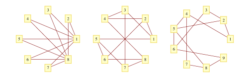
Figure 1: (L): The graph $W$. There is PST between vertices $1$ and $8$. The spectrum of $W$ is not integral. (C): The 3-dimensional cube. There is PST between vertices $1$ and $8$. These vertices are antipodal and at distance $3$. (R): The graph $P_{3}^{\times 2}$. Note that the graph has vertices of degree two and three. There is PST between the vertices $1$ and $9$. These vertices are antipodal and at distance four.

It is an open problem to prove that $P_{2}^{\times 3}$ is the only connected cubic graph with PST.

Conjecture. $\mathcal{G}_{D,3}^{R}=\{P_{2}^{\times 3}\}$ if $D=3$ and $\mathcal{G}_{D,3}^{R}=\emptyset$, otherwise.

Periodicity is not necessary for PST. There are examples of regular graphs that are not periodic but have PST ru .

II Proof of the theorem

II.1 Integral graphs

The spectrum of a graph $G$ is the multiset $\{\lambda_{1}^{[m_{1}]}(G),\lambda_{2}^{[m_{2}]}(G),...,\lambda_{r}^{[m_{r}]}(G)\}$ of the eigenvalues of $A(G)$. The index $[m_{i}]$ in $\lambda_{i}^{[m_{i}]}(G)$ denotes the multiplicity of the eigenvalue $\lambda_{i}(G)$. For example, the spectrum of the complete graph on four vertices, $K_{4}$, is $\{3,-1^{[3]}\}$. A graph is said to be integral if its eigenvalues are integers. There is basically one survey on this area ba . See also cds for the relevant terminology and ah for a nontrivial upper bounds on the total number of integral graphs with $n$ vertices. There are a few general results that establish a relation between PST and integral graphs god . The next statement is directly useful to our purposes:

P0.

A connected regular graph is periodic if and only if it is integral (Corollary 2.3 god ).

The converse is not necessarily true. This fact can be observed in the examples discussed below. Moreover, integer eigenvalues have a weaker role in nonregular graphs. Let us consider, for instance, a graph $W$ with eight vertices $\{1,2,...,8\}$ and set of edges $E(W)=\{\{1,i\},\{j,8\}:2\leq i,j\leq 7;\}$ (see Fig. 1). The unitary governing the dynamics in $W$ is defined by

−isin(23t)/23,if {i,j}∈E(W);cos(3t)2,If i=j=1,8;(5+cos(23t))/6,if i=j≠1,8;−sin(3t)2,otherwise.[U_{W}\left(t\right)]_{i,j}=\left\{\begin{tabular}[c]{rr}$-\sin\left(\sqrt{3}t\right)^{2},$&if $i=1$ and $j=8$ or \emph{viz.};\\ $-i\sin\left(2\sqrt{3}t\right)/2\sqrt{3},$&if $\{i,j\}\in E(W)$;\\ $\cos\left(\sqrt{3}t\right)^{2},$&If $i=j=1,8$;\\ $\left(5+\cos\left(2\sqrt{3}t\right)\right)/6,$&if $i=j\neq 1,8$;\\ $-\sin\left(\sqrt{3}t\right)^{2},$&otherwise.\end{tabular}\ \right.

-sin(3t)2,if =i1 and =j8 or viz.;

There is PST between vertices $1$ and $8$, because $[U_{W}\left(\pi/2\sqrt{3}\right)]_{1,8}=-\sin\left(3\pi/2\right)^{2}=-1$. At the same time, the $6\times 6$ submatrix of $U_{W}\left(\pi/2\sqrt{3}\right)$, excluding the first/last row/column, is $2/3$ in the diagonal and $-1/3$ off-diagonal. The spectrum of $W$ is $\{\pm 2\sqrt{3},0^{\left[6\right]}\}$. Thus, $W$ is not an integral graph.

We shall be interested in a special family of graphs. A cubic graph is a $3$-regular graph. All cubic integral graphs have been classified and explicitly constructed bc ; s . In particular,

P1.

There are exactly thirteen connected cubic integral graphs.

On the light of the statements P0 and P1, a proof of the theorem can be obtained via a case by case analysis. As we have seen, and this is an already known fact, the $3$-dimensional cube, $P_{2}^{\times 3}$, has PST between its antipodal vertices. These are vertices at distance three. We shall verify that none of the remaining twelve connected, cubic integral graphs affords PST. All graphs considered in this section are periodic.

II.2 The complete graph $K_{4}$, the complete bipartite graph $K_{3,3}$, and two connected copies of $K_{2,3}$

A complete graph on $n$ vertices is a graph $K_{n}=\left(\{1,...,n\},E\right)$, where $E(K_{n})=\{\{i,j\}:1\leq i,j\leq n\}$. The $ij$-entries of $U_{K_{4}}$ are given by

$$[U_{K_{4}}(t)]_{i,j}=\left\{\begin{tabular}[c]{rr}$\left(3\cos\left(t\right)+\cos\left(3t\right)+4i\sin\left(t\right)^{3}\right)/4,$&if $i=j$;\\ $\cos\left(t\right)\sin\left(t\right)\left(-i\cos\left(t\right)-\sin\left(t\right)\right),$&if $i\neq j$.\end{tabular}\ \right.$$

Then $\max_{t\in\mathbb{R}^{+}}\left([U_{K_{4}}(t)]_{i,i}\right)=f_{U_{K_{4}}}\left(i,i;\pi/2\right)=1$, for $1\leq i\leq 4$; for every pair of vertices $i$ and $j$, $\max_{t\in\mathbb{R}^{+}}\left([U_{K_{4}}(t)]_{i,j}\right)=f_{U_{K_{4}}}\left(i,j;\pi/4\right)=1/2$. Note that

$$[U_{K_{4}}(\pi/4)]_{i,j}=\dfrac{1}{\sqrt{2}}\left\{\begin{tabular}[c]{rr}$(1+i)/2,$&if $i=j$;\\ $-(1+i)/2,$&if $i\neq j$.\end{tabular}\ \right.$$

gives a complex Hadamard matrix.

A graph $G=(V=V_{1}\cup V_{2},E)$ is bipartite if each vertex in $V_{1}$ is adjacent to vertices in $V_{2}$ only and viz. A complete bipartite graph is a bipartite graph $K_{q,p}=(V=V_{1}\cup V_{2},E)$ such that $\left|V_{1}\right|=p$, $\left|V_{2}\right|=q$ and $E=\{\{i,j\}:i\in V_{1}$ and $j\in V_{2}\}$. The graph $K_{3,3}$ is on six vertices; $V(K_{3,3})=\{A,B\}$, with $\left|A\right|=\left|B\right|=3$. By definition, $\{i,j\}\in E(K_{3,3})$ if and only if $i\in A$ and $j\in B$. The spectrum of $K_{3,3}$ is $\{\pm 3,0^{[4]}\}$ and dia$\left(K_{3,3}\right)=2$. The $ij$-entries of $U_{K_{3,3}}$ are as follows:

$$[U_{K_{3,3}}(t)]_{i,j}=\left\{\begin{tabular}[c]{rr}$\left(2+\cos\left(3t\right)\right)/3,$&$i=j;$\\ $\left(-1+\cos\left(3t\right)\right)/3,$&$\{i,j\}\notin E(K_{3,3});$\\ $-i\sin\left(3t\right)/3,$&$\{i,j\}\in E(K_{3,3}).$\end{tabular}\right.$$

Hence, $\max_{t\in\mathbb{R}^{+}}\left(\left|[U_{K_{3,3}}(t)]_{i,i}\right|\right)=f_{U_{K_{3,3}}}\left(i,i;2\pi/3\right)=1$, for $1\leq i\leq 6$. For the off-diagonal entries, we need to distinguish two cases: (i) $\max_{t\in\mathbb{R}^{+}}\left(\left|[U_{K_{3,3}}(t)]_{i,j}\right|\right)=f_{U_{K_{3,3}}}\left(i,j;\pi/3\right)=2/3$, if $i,j\in A$ or $i,j\in B$; (ii) $\max_{t\in\mathbb{R}^{+}}\left([\left|U_{K_{3,3}}(t)]_{i,j}\right|\right)=f_{U_{K_{3,3}}}\left(i,j;\pi/6\right)=1/3$, if $i\in A$ and $j\in B$. When $t=\pi/2$,

$$[U_{K_{3,3}}(\pi/2)]_{i,j}=\left\{\begin{tabular}[c]{rr}$2/3,$&$i=j;$\\ $-1/3,$&$\{i,j\}\notin E(K_{3,3});$\\ $i/3,$&$\{i,j\}\in E(K_{3,3}).$\end{tabular}\right.$$

Let $DK_{2,3}$ be the graph on ten vertices obtained from two disjoint copies of $K_{2,3}$, say $K_{2,3}^{1}$ and $K_{2,3}^{2}$, by adding three edges between the vertices of degree two in $K_{2,3}^{1}$ and $K_{2,3}^{2}$. The spectrum of $DK_{2,3}$ is $\{\pm 3,\pm 2,\pm 1^{[2]},0^{[2]}\}$ and dia$\left(DK_{2,3}\right)=3$. The structure of $U_{DK_{3,3}}$ consists of various kind of entries:

$$U_{DK_{2,3}}(t)=\begin{tabular}[c]{cccccccccc}$a_{1}$&$a_{2}$&$a_{3}$&$a_{3}$&$a_{3}$&$a_{4}$&$a_{4}$&$a_{4}$&$a_{5}$&$a_{5}$\\ $a_{2}$&$a_{1}$&$a_{3}$&$a_{3}$&$a_{3}$&$a_{4}$&$a_{4}$&$a_{4}$&$a_{5}$&$a_{5}$\\ \cline{3-8}\cr\cline{3-8}\cr$a_{3}$&$a_{3}$&\vrule\lx@intercol\hfil$a_{6}$\hfil\lx@intercol &$a_{7}$&\lx@intercol\hfil$a_{7}$\hfil\lx@intercol\vrule\lx@intercol &$a_{8}$&$a_{9}$&\lx@intercol\hfil$a_{9}$\hfil\lx@intercol\vrule\lx@intercol &\vrule\lx@intercol\hfil$a_{4}$\hfil\lx@intercol &$a_{4}$\\ $a_{3}$&$a_{3}$&\vrule\lx@intercol\hfil$a_{7}$\hfil\lx@intercol &$a_{6}$&\lx@intercol\hfil$a_{7}$\hfil\lx@intercol\vrule\lx@intercol &$a_{9}$&$a_{8}$&\lx@intercol\hfil$a_{9}$\hfil\lx@intercol\vrule\lx@intercol &\vrule\lx@intercol\hfil$a_{4}$\hfil\lx@intercol &$a_{4}$\\ $a_{3}$&$a_{3}$&\vrule\lx@intercol\hfil$a_{7}$\hfil\lx@intercol &$a_{7}$&\lx@intercol\hfil$a_{6}$\hfil\lx@intercol\vrule\lx@intercol &$a_{9}$&$a_{9}$&\lx@intercol\hfil$a_{8}$\hfil\lx@intercol\vrule\lx@intercol &\vrule\lx@intercol\hfil$a_{4}$\hfil\lx@intercol &$a_{4}$\\ \cline{3-8}\cr\cline{3-8}\cr$a_{4}$&$a_{4}$&\vrule\lx@intercol\hfil$a_{8}$\hfil\lx@intercol &$a_{9}$&\lx@intercol\hfil$a_{9}$\hfil\lx@intercol\vrule\lx@intercol &\vrule\lx@intercol\hfil$a_{6}$\hfil\lx@intercol &$a_{7}$&$a_{7}$&\vrule\lx@intercol\hfil$a_{3}$\hfil\lx@intercol &$a_{3}$\\ $a_{4}$&$a_{4}$&\vrule\lx@intercol\hfil$a_{9}$\hfil\lx@intercol &$a_{8}$&\lx@intercol\hfil$a_{9}$\hfil\lx@intercol\vrule\lx@intercol &\vrule\lx@intercol\hfil$a_{7}$\hfil\lx@intercol &$a_{6}$&$a_{7}$&\vrule\lx@intercol\hfil$a_{3}$\hfil\lx@intercol &$a_{3}$\\ $a_{4}$&$a_{4}$&\vrule\lx@intercol\hfil$a_{9}$\hfil\lx@intercol &$a_{9}$&\lx@intercol\hfil$a_{8}$\hfil\lx@intercol\vrule\lx@intercol &\vrule\lx@intercol\hfil$a_{7}$\hfil\lx@intercol &$a_{7}$&$a_{6}$&\vrule\lx@intercol\hfil$a_{3}$\hfil\lx@intercol &$a_{3}$\\ \cline{3-5}\cr\cline{3-8}\cr\cline{6-8}\cr$a_{5}$&$a_{5}$&$a_{4}$&$a_{4}$&$a_{4}$&$a_{3}$&$a_{3}$&$a_{3}$&$a_{1}$&$a_{2}$\\ $a_{5}$&$a_{5}$&$a_{4}$&$a_{4}$&$a_{4}$&$a_{3}$&$a_{3}$&$a_{3}$&$a_{2}$&$a_{1}$\end{tabular}\text{ },$$

where

$$a_{1}=\left(5+3\cos\left(2t\right)+2\cos\left(3t\right)\right)/10,$$

By considering $a_{1}$ and $a_{6}$, we can see that $\max_{t\in\mathbb{R}^{+}}\left(\left|[U_{DK_{2,3}}(t)]_{i,i}\right|\right)=f_{DK_{2,3}}\left(i,i;2\pi\right)=1$, for every $i$. However, $\max_{1\leq j\leq 9;j\neq 1,6}\max_{t\in\mathbb{R}^{+}}\left(\left|a_{j}\right|\right)=\left(5-5\left(-1-\sqrt{5}\right)/4\right)/10\approx 0.9$. The maximum is attained by $a_{2}$ for $t=2\pi/5$. The segments in the matrix $U_{DK_{3,3}}(t)$ help visualizing its structure and these do not have a mathematical meaning. We shall make a consistent use of this graphic tool also in the next cases. The graphs $K_{3,3}$ and $DK_{2,3}$ are in Fig. (2).

II.3 The graphs $C_{3}+K_{2}$ and $C_{6}+K_{2}$

The (Cartesian) sum $G=G_{1}+G_{2}=(V,E)$ of two graphs $G_{1}=\left(V_{1},E_{1}\right)$ and $G_{2}=\left(V_{2},E_{2}\right)$ has set of vertices $V(G)=V(G_{1})\times V(G_{2})$ and $\{\{i,j\},\{k,l\}\}\in E\left(G\right)$ if (i) $\{i,k\}\in E(G_{1})$ or (ii) $\{j,l\}\in E(G_{2})$ ore . We denote by $C_{n}$ the $n$-cycle: $V(C_{n})=\{1,2,...,n\}$ and $\{i,\left(i+1\right)\operatorname{mod}n\}\in E(C_{n})$.

The graph $C_{3}+K_{2}$ has two cycles of length three and it can be drawn as a prism with triangular basis. It is the undirected version the Cayley digraph of the dihedral group $D_{6}$ generated by the standard set. Its spectrum is $\{3,1,0^{[2]},-2^{[2]}\}$. Given the symmetry, the unitary matrix has a neat structure:

$$U_{C_{3}+K_{2}}(t)=\begin{tabular}[c]{lll|lll}$a_{1}$&$a_{2}$&$a_{2}$&$a_{3}$&$a_{4}$&$a_{4}$\\ $a_{2}$&$a_{1}$&$a_{2}$&$a_{4}$&$a_{3}$&$a_{4}$\\ $a_{2}$&$a_{2}$&$a_{1}$&$a_{4}$&$a_{4}$&$a_{3}$\\ \hline\cr$a_{3}$&$a_{4}$&$a_{4}$&$a_{1}$&$a_{2}$&$a_{2}$\\ $a_{4}$&$a_{3}$&$a_{4}$&$a_{2}$&$a_{1}$&$a_{2}$\\ $a_{4}$&$a_{4}$&$a_{3}$&$a_{2}$&$a_{2}$&$a_{1}$\end{tabular}\text{ },$$

with

$$a_{1}=\left(2+e^{-it}+2e^{2it}+e^{-3it}\right)/6,$$

From this, $\max_{2\leq j\leq 4}\max_{t\in\mathbb{R}^{+}}\left(\left|a_{j}\right|\right)\approx 0.9$, for $j=3$ and $t=\sqrt{3}+\pi/17$.

The graph $C_{6}+K_{2}$ is on twelve vertices. It has two cycles of length six and it can be drawn as a prism with hexagonal basis. In fact, in analogy with $C_{3}+K_{2}$, it is the undirected version the Cayley digraph of the dihedral group $D_{12}$ generated by the standard set. As we have done for the other cases, we explicitly write down the unitary matrix. Let

a2a1a2a3a4a3a3a2a1a2a3a4a4a3a2a1a2a3a3a4a3a2a1a2a2a3a4a3a2a1andB=

a1a2a3a4a3a2

a5	a6	a7	a8	a7	a6
a6	a5	a6	a7	a8	a7
a7	a6	a5	a6	a7	a8
a8	a7	a6	a5	a6	a7
a7	a8	a7	a6	a5	a6
a6	a7	a8	a7	a6	a5

 .𝐴fragments a1 a2 a3 a4 a3 a2fragmentsa2fragmentsa1fragmentsa2fragmentsa3fragmentsa4fragmentsa3fragmentsa3fragmentsa2fragmentsa1fragmentsa2fragmentsa3fragmentsa4fragmentsa4fragmentsa3fragmentsa2fragmentsa1fragmentsa2fragmentsa3fragmentsa3fragmentsa4fragmentsa3fragmentsa2fragmentsa1fragmentsa2fragmentsa2fragmentsa3fragmentsa4fragmentsa3fragmentsa2fragmentsa1and𝐵

a5	a6	a7	a8	a7	a6
a6	a5	a6	a7	a8	a7
a7	a6	a5	a6	a7	a8
a8	a7	a6	a5	a6	a7
a7	a8	a7	a6	a5	a6
a6	a7	a8	a7	a6	a5

 \begin{array}[c]{ccc}A=\begin{tabular}[c]{lll|lll}$a_{1}$&$a_{2}$&$a_{3}$&$a_{4}$&$a_{3}$&$a_{2}$\\ $a_{2}$&$a_{1}$&$a_{2}$&$a_{3}$&$a_{4}$&$a_{3}$\\ $a_{3}$&$a_{2}$&$a_{1}$&$a_{2}$&$a_{3}$&$a_{4}$\\ \hline\cr$a_{4}$&$a_{3}$&$a_{2}$&$a_{1}$&$a_{2}$&$a_{3}$\\ $a_{3}$&$a_{4}$&$a_{3}$&$a_{2}$&$a_{1}$&$a_{2}$\\ $a_{2}$&$a_{3}$&$a_{4}$&$a_{3}$&$a_{2}$&$a_{1}$\end{tabular}&\text{and}&B=\begin{tabular}[c]{lll|lll}$a_{5}$&$a_{6}$&$a_{7}$&$a_{8}$&$a_{7}$&$a_{6}$\\ $a_{6}$&$a_{5}$&$a_{6}$&$a_{7}$&$a_{8}$&$a_{7}$\\ $a_{7}$&$a_{6}$&$a_{5}$&$a_{6}$&$a_{7}$&$a_{8}$\\ \hline\cr$a_{8}$&$a_{7}$&$a_{6}$&$a_{5}$&$a_{6}$&$a_{7}$\\ $a_{7}$&$a_{8}$&$a_{7}$&$a_{6}$&$a_{5}$&$a_{6}$\\ $a_{6}$&$a_{7}$&$a_{8}$&$a_{7}$&$a_{6}$&$a_{5}$\end{tabular}\text{ }.\end{array}

Then

$$U_{C_{6}+K_{2}}(t)=\left[\begin{array}[c]{cc}A&B\\ B&A\end{array}\right],$$

and

$$a_{1}=\left(2+\cos\left(t\right)+2\cos\left(2t\right)+\cos\left(3t\right)\right)/6,$$

For $j\neq 1$,

$$\max_{t\in\mathbb{R}^{+}}\left(\left|a_{j}\right|\right)\left\{\begin{tabular}[c]{rr}$\approx 21/50,$&$j=2$ and $t\approx\pi/6;$\\ $=2/3,$&$j=3$ and $t=\pi;$\\ $\approx 29/50,$&$j=4$ and $t=77/20$\\ $\approx 9/20,$&$j=5$ and $t=19/10;$\\ $\approx 1/2,$&$j=6$ and $t\approx 1.21;$\\ $\approx 9/25,$&$j=7$ and $t\approx 1.35;$\\ $\approx 64/81,$&$j=8$ and $t\approx 1.9.$\end{tabular}\right.$$

The graphs $C_{3}+K_{2}$, and $C_{6}+K_{2}$ are represented in Fig. (2).

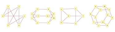
Figure 2: From the left: The complete bipartite graph $K_{3,3}$. The graph obtained by connecting together two copies of $K_{2,3}$. The graph $C_{3}+K_{2}$. The graph $C_{6}+K_{2}$. Although periodic, none of these graphs has PST.

II.4 The Petersen graph, a graph on ten vertices, and $L\left(S\left(K_{4}\right)\right)$

The Petersen graph, $P$, illustrated in Fig. (3), is one of the best-studied single objects in the graph-theoretic literature. The Petersen graph has two cycles of length five. It is vertex-transitive but not a Cayley graph, with spectrum $\{3,1^{[4]},-2^{[4]}\}$ and dia$\left(P\right)=3$. It is strongly regular with parameters $(10,3,0,1)$. The symmetry appears also in $U_{P}(t)$, which reflects faithfully the structure of $P$:

$$U_{P}(t)=\begin{tabular}[c]{lllll|lllll}$a_{1}$&$a_{2}$&$a_{3}$&$a_{3}$&$a_{2}$&$a_{2}$&$a_{3}$&$a_{3}$&$a_{3}$&$a_{3}$\\ $a_{2}$&$a_{1}$&$a_{2}$&$a_{3}$&$a_{3}$&$a_{3}$&$a_{2}$&$a_{3}$&$a_{3}$&$a_{3}$\\ $a_{3}$&$a_{2}$&$a_{1}$&$a_{2}$&$a_{3}$&$a_{3}$&$a_{3}$&$a_{2}$&$a_{3}$&$a_{3}$\\ $a_{3}$&$a_{3}$&$a_{2}$&$a_{1}$&$a_{2}$&$a_{3}$&$a_{3}$&$a_{3}$&$a_{2}$&$a_{3}$\\ $a_{2}$&$a_{3}$&$a_{3}$&$a_{2}$&$a_{1}$&$a_{3}$&$a_{3}$&$a_{3}$&$a_{3}$&$a_{2}$\\ \hline\cr$a_{2}$&$a_{3}$&$a_{3}$&$a_{3}$&$a_{3}$&$a_{1}$&$a_{3}$&$a_{2}$&$a_{2}$&$a_{3}$\\ $a_{3}$&$a_{2}$&$a_{3}$&$a_{3}$&$a_{3}$&$a_{3}$&$a_{1}$&$a_{3}$&$a_{2}$&$a_{2}$\\ $a_{3}$&$a_{3}$&$a_{2}$&$a_{3}$&$a_{3}$&$a_{2}$&$a_{3}$&$a_{1}$&$a_{3}$&$a_{2}$\\ $a_{3}$&$a_{3}$&$a_{3}$&$a_{2}$&$a_{3}$&$a_{2}$&$a_{2}$&$a_{3}$&$a_{1}$&$a_{3}$\\ $a_{3}$&$a_{3}$&$a_{3}$&$a_{3}$&$a_{2}$&$a_{3}$&$a_{2}$&$a_{2}$&$a_{3}$&$a_{1}$\end{tabular}\text{ },$$

where

$$a_{1}=e^{-3it}\left(1+5e^{2it}+4e^{5it}\right)/10,$$

Thus, $\max_{j=2,3}\max_{t\in\mathbb{R}^{+}}\left(\left|a_{j}\right|\right)=8/15$, for $j=2$ and $t=\pi$. More generally, $[U_{P}(\pi)]_{i,j}=-1/5$ if $i=j$; $2/15$ if $\{i,j\}\notin E(P)$ and $-8/15$, otherwise.

There is another cubic integral graph on ten vertices, obtained by replacing with triangles two nonadjacent vertices of $K_{3,3}$. Denoted by $Z$, it has spectrum $\{3,2,1^{[3]},-1^{[2]},-2^{[3]}\}$. Fig. (3) contains a drawing. The unitary matrix obtained from $Z$ is

$$U_{Z}(t)=\begin{tabular}[c]{llll|llllll}\cline{1-4}\cr\vrule\lx@intercol$a_{1}$\hfil\lx@intercol &$a_{2}$&$a_{2}$&$a_{2}$&$a_{3}$&$a_{3}$&$a_{3}$&$a_{3}$&$a_{3}$&$a_{3}$\\ \vrule\lx@intercol$a_{2}$\hfil\lx@intercol &$a_{1}$&$a_{3}$&$a_{3}$&$a_{3}$&$a_{3}$&$a_{2}$&$a_{3}$&$a_{2}$&$a_{3}$\\ \vrule\lx@intercol$a_{2}$\hfil\lx@intercol &$a_{3}$&$a_{1}$&$a_{3}$&$a_{2}$&$a_{2}$&$a_{3}$&$a_{3}$&$a_{3}$&$a_{3}$\\ \vrule\lx@intercol$a_{2}$\hfil\lx@intercol &$a_{3}$&$a_{3}$&$a_{1}$&$a_{3}$&$a_{3}$&$a_{3}$&$a_{2}$&$a_{3}$&$a_{2}$\\ \hline\cr$a_{3}$&$a_{3}$&$a_{2}$&$a_{3}$&$a_{5}$&$a_{4}$&$a_{6}$&$a_{6}$&$a_{7}$&\lx@intercol$a_{7}$\hfil\lx@intercol\vrule\lx@intercol\\ $a_{3}$&$a_{3}$&$a_{2}$&$a_{3}$&$a_{4}$&$a_{5}$&$a_{7}$&$a_{7}$&$a_{6}$&\lx@intercol$a_{6}$\hfil\lx@intercol\vrule\lx@intercol\\ $a_{3}$&$a_{2}$&$a_{3}$&$a_{3}$&$a_{6}$&$a_{7}$&$a_{5}$&$a_{6}$&$a_{4}$&\lx@intercol$a_{7}$\hfil\lx@intercol\vrule\lx@intercol\\ $a_{3}$&$a_{3}$&$a_{3}$&$a_{2}$&$a_{6}$&$a_{7}$&$a_{6}$&$a_{5}$&$a_{7}$&\lx@intercol$a_{4}$\hfil\lx@intercol\vrule\lx@intercol\\ $a_{3}$&$a_{2}$&$a_{3}$&$a_{3}$&$a_{7}$&$a_{6}$&$a_{4}$&$a_{7}$&$a_{5}$&\lx@intercol$a_{6}$\hfil\lx@intercol\vrule\lx@intercol\\ $a_{3}$&$a_{3}$&$a_{3}$&$a_{2}$&$a_{7}$&$a_{6}$&$a_{7}$&$a_{4}$&$a_{6}$&\lx@intercol$a_{5}$\hfil\lx@intercol\vrule\lx@intercol\\ \cline{5-10}\cr\end{tabular}\text{ .}$$

The entries are

$$a_{1}=e^{-3it}\left(1+5e^{2it}+4e^{5it}\right)/10,$$

We then obtain $\max_{1\leq j\leq 9;j\neq 1,5}\max_{t\in\mathbb{R}^{+}}\left(\left|a_{j}\right|\right)\approx 0.85$, for $j=4$ and $t\approx\pi-5/6$. Note that $a_{1}$, $a_{2}$, and $a_{3}$ give the same dynamics as the Petersen graph.

The graph $X=L\left(S\left(K_{4}\right)\right)$ is constructed by replacing each vertex of $K_{4}$ with a triangle (see Fig. (3)). The triangles are then connected by independent edges. The notation indicates the line graph of the $K_{4}$ subdivision. Its spectrum is $\{3,\pm 2^{[3]},0^{[2]},-1^{[3]}\}$ and dia$\left(X\right)=3$. The unitary has some symmetry:

$$U_{X}(t)=\begin{tabular}[c]{llllllllllll}\cline{1-3}\cr\cline{8-8}\cr\vrule\lx@intercol$a_{1}$\hfil\lx@intercol &$a_{2}$&\lx@intercol$a_{2}$\hfil\lx@intercol\vrule\lx@intercol &$a_{4}$&$a_{5}$&$a_{6}$&$a_{4}$&\vrule\lx@intercol$a_{3}$\hfil\lx@intercol &\vrule\lx@intercol$a_{4}$\hfil\lx@intercol &$a_{4}$&$a_{6}$&$a_{5}$\\ \cline{4-4}\cr\cline{8-8}\cr\vrule\lx@intercol$a_{2}$\hfil\lx@intercol &$a_{1}$&\lx@intercol$a_{2}$\hfil\lx@intercol\vrule\lx@intercol &\lx@intercol$a_{3}$\hfil\lx@intercol\vrule\lx@intercol &$a_{4}$&$a_{4}$&$a_{5}$&$a_{4}$&$a_{6}$&$a_{4}$&$a_{5}$&$a_{6}$\\ \cline{4-4}\cr\cline{10-10}\cr\vrule\lx@intercol$a_{2}$\hfil\lx@intercol &$a_{2}$&\lx@intercol$a_{1}$\hfil\lx@intercol\vrule\lx@intercol &$a_{4}$&$a_{6}$&$a_{5}$&$a_{4}$&$a_{4}$&$a_{5}$&\vrule\lx@intercol$a_{3}$\hfil\lx@intercol &\vrule\lx@intercol$a_{4}$\hfil\lx@intercol &$a_{4}$\\ \cline{1-6}\cr\cline{2-2}\cr\cline{10-10}\cr$a_{4}$&\vrule\lx@intercol$a_{3}$\hfil\lx@intercol &\vrule\lx@intercol$a_{4}$\hfil\lx@intercol &\vrule\lx@intercol$a_{1}$\hfil\lx@intercol &$a_{2}$&\lx@intercol$a_{2}$\hfil\lx@intercol\vrule\lx@intercol &$a_{4}$&$a_{5}$&$a_{6}$&$a_{5}$&$a_{4}$&$a_{6}$\\ \cline{2-2}\cr\cline{7-7}\cr$a_{5}$&$a_{4}$&$a_{6}$&\vrule\lx@intercol$a_{2}$\hfil\lx@intercol &$a_{1}$&\lx@intercol$a_{2}$\hfil\lx@intercol\vrule\lx@intercol &\lx@intercol$a_{3}$\hfil\lx@intercol\vrule\lx@intercol &$a_{4}$&$a_{4}$&$a_{6}$&$a_{4}$&$a_{5}$\\ \cline{7-7}\cr\cline{11-11}\cr$a_{6}$&$a_{4}$&$a_{5}$&\vrule\lx@intercol$a_{2}$\hfil\lx@intercol &$a_{2}$&\lx@intercol$a_{1}$\hfil\lx@intercol\vrule\lx@intercol &$a_{4}$&$a_{6}$&$a_{5}$&$a_{4}$&\vrule\lx@intercol$a_{3}$\hfil\lx@intercol &\vrule\lx@intercol$a_{4}$\hfil\lx@intercol\\ \cline{4-9}\cr\cline{5-5}\cr\cline{11-11}\cr$a_{4}$&$a_{5}$&$a_{6}$&$a_{4}$&\vrule\lx@intercol$a_{3}$\hfil\lx@intercol &\vrule\lx@intercol$a_{4}$\hfil\lx@intercol &\vrule\lx@intercol$a_{1}$\hfil\lx@intercol &$a_{2}$&\lx@intercol$a_{2}$\hfil\lx@intercol\vrule\lx@intercol &$a_{6}$&$a_{5}$&$a_{4}$\\ \cline{1-1}\cr\cline{5-5}\cr\vrule\lx@intercol$a_{3}$\hfil\lx@intercol &\vrule\lx@intercol$a_{4}$\hfil\lx@intercol &$a_{4}$&$a_{5}$&$a_{4}$&$a_{6}$&\vrule\lx@intercol$a_{2}$\hfil\lx@intercol &$a_{1}$&\lx@intercol$a_{2}$\hfil\lx@intercol\vrule\lx@intercol &$a_{5}$&$a_{6}$&$a_{4}$\\ \cline{1-1}\cr\cline{12-12}\cr$a_{4}$&$a_{6}$&$a_{5}$&$a_{6}$&$a_{4}$&$a_{5}$&\vrule\lx@intercol$a_{2}$\hfil\lx@intercol &$a_{2}$&\lx@intercol$a_{1}$\hfil\lx@intercol\vrule\lx@intercol &$a_{4}$&$a_{4}$&\vrule\lx@intercol$a_{3}$\hfil\lx@intercol\vrule\lx@intercol\\ \cline{3-3}\cr\cline{7-12}\cr\cline{12-12}\cr$a_{4}$&$a_{4}$&\vrule\lx@intercol$a_{3}$\hfil\lx@intercol &\vrule\lx@intercol$a_{5}$\hfil\lx@intercol &$a_{6}$&$a_{4}$&$a_{6}$&$a_{5}$&$a_{4}$&\vrule\lx@intercol$a_{1}$\hfil\lx@intercol &$a_{2}$&\lx@intercol$a_{2}$\hfil\lx@intercol\vrule\lx@intercol\\ \cline{3-3}\cr\cline{6-6}\cr$a_{6}$&$a_{5}$&$a_{4}$&$a_{4}$&$a_{4}$&\vrule\lx@intercol$a_{3}$\hfil\lx@intercol &\vrule\lx@intercol$a_{5}$\hfil\lx@intercol &$a_{6}$&$a_{4}$&\vrule\lx@intercol$a_{2}$\hfil\lx@intercol &$a_{1}$&\lx@intercol$a_{2}$\hfil\lx@intercol\vrule\lx@intercol\\ \cline{6-6}\cr\cline{9-9}\cr$a_{5}$&$a_{6}$&$a_{4}$&$a_{6}$&$a_{5}$&$a_{4}$&$a_{4}$&$a_{4}$&\vrule\lx@intercol$a_{3}$\hfil\lx@intercol &\vrule\lx@intercol$a_{2}$\hfil\lx@intercol &$a_{2}$&\lx@intercol$a_{1}$\hfil\lx@intercol\vrule\lx@intercol\\ \cline{9-9}\cr\cline{9-12}\cr\end{tabular}\ ,$$

with

$$a_{1}=\left(2+3e^{it}+3e^{-2it}+3e^{2it}+e^{-3it}\right)/12,$$

  

For $j\neq 1$,

$$\max_{t\in\mathbb{R}^{+}}\left(\left|a_{j}\right|\right)\left\{\begin{tabular}[c]{rr}$\approx 1/2,$&$j=2$ and $t\approx\pi/4;$\\ $\approx 1/2,$&$j=3$ and $t\approx\pi/4;$\\ $\approx 1/4,$&$j=4$ and $t\approx 6/5;$\\ $=2/3,$&$j=5$ and $t=\pi;$\\ $=\sqrt{3}/4,$&$j=6$ and $t=2\pi/3.$\end{tabular}\ \right.$$

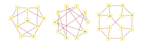
Figure 3: (L): The Petersen graph. (C): The graph $Z$ on ten vertices. (R): The graph $L\left(S\left(K_{4}\right)\right)$ on twelve vertices. These graphs are periodic without PST.

II.5 The Desargues graph and its cospectral mate

The bipartite double cover of the Petersen graph is called Desargues graph. There are many different notations for this graph. We adopt $H_{5,2}$. The Desargues graph is on twenty vertices and its spectrum is $\left\{\pm 3,\pm 2^{[4]},\pm 1^{[5]}\right\}$. The graph $H_{5,2}$ has a cospectral mate, which we will denote by $H_{5,2}^{\prime}$. This is a nonisomorphic graph with the same spectrum. Two graphs $G$ and $H$ are said to isomorphic if there is a permutation matrix $Q$ such that $QA(G)Q^{T}=A(H)$. It is clear that two isomorphic graphs have the same spectrum. The converse is not necessarily true. Indeed, $H_{5,2}$ and $H_{5,2}^{\prime}$ are a counterexample. The graphs $H_{5,2}$ and $H_{5,2}^{\prime}$ are drawn in Fig. (4). Let us define the arrays

$$A=\begin{tabular}[c]{llllllllll}$a_{1}$&$a_{2}$&$a_{2}$&$a_{2}$&$a_{3}$&$a_{2}$&$a_{2}$&$a_{2}$&$a_{3}$&$a_{3}$\\ $a_{2}$&$a_{1}$&$a_{2}$&$a_{2}$&$a_{2}$&$a_{3}$&$a_{3}$&$a_{2}$&$a_{2}$&$a_{3}$\\ $a_{2}$&$a_{2}$&$a_{1}$&$a_{3}$&$a_{2}$&$a_{2}$&$a_{2}$&$a_{3}$&$a_{2}$&$a_{3}$\\ $a_{2}$&$a_{2}$&$a_{3}$&$a_{1}$&$a_{2}$&$a_{2}$&$a_{3}$&$a_{2}$&$a_{3}$&$a_{2}$\\ $a_{3}$&$a_{2}$&$a_{2}$&$a_{2}$&$a_{1}$&$a_{2}$&$a_{3}$&$a_{3}$&$a_{2}$&$a_{2}$\\ $a_{2}$&$a_{3}$&$a_{2}$&$a_{2}$&$a_{2}$&$a_{1}$&$a_{2}$&$a_{3}$&$a_{3}$&$a_{2}$\\ $a_{2}$&$a_{3}$&$a_{2}$&$a_{3}$&$a_{3}$&$a_{2}$&$a_{1}$&$a_{2}$&$a_{2}$&$a_{2}$\\ $a_{2}$&$a_{2}$&$a_{3}$&$a_{2}$&$a_{3}$&$a_{3}$&$a_{2}$&$a_{1}$&$a_{2}$&$a_{2}$\\ $a_{3}$&$a_{2}$&$a_{2}$&$a_{3}$&$a_{2}$&$a_{3}$&$a_{2}$&$a_{2}$&$a_{1}$&$a_{2}$\\ $a_{3}$&$a_{3}$&$a_{3}$&$a_{2}$&$a_{2}$&$a_{2}$&$a_{2}$&$a_{2}$&$a_{2}$&$a_{1}$\end{tabular},$$

$$B=\begin{tabular}[c]{llllllllll}$a_{4}$&$a_{4}$&$a_{4}$&$a_{8}$&$a_{8}$&$a_{8}$&$a_{8}$&$a_{8}$&$a_{8}$&$a_{7}$\\ $a_{4}$&$a_{8}$&$a_{8}$&$a_{4}$&$a_{8}$&$a_{4}$&$a_{8}$&$a_{8}$&$a_{7}$&$a_{8}$\\ $a_{4}$&$a_{8}$&$a_{8}$&$a_{8}$&$a_{7}$&$a_{8}$&$a_{4}$&$a_{4}$&$a_{8}$&$a_{8}$\\ $a_{5}$&$a_{4}$&$a_{6}$&$a_{4}$&$a_{8}$&$a_{6}$&$a_{6}$&$a_{4}$&$a_{8}$&$a_{8}$\\ $a_{6}$&$a_{4}$&$a_{5}$&$a_{8}$&$a_{4}$&$a_{6}$&$a_{6}$&$a_{8}$&$a_{4}$&$a_{8}$\\ $a_{8}$&$a_{8}$&$a_{4}$&$a_{8}$&$a_{4}$&$a_{4}$&$a_{8}$&$a_{7}$&$a_{8}$&$a_{8}$\\ $a_{8}$&$a_{8}$&$a_{4}$&$a_{7}$&$a_{8}$&$a_{8}$&$a_{4}$&$a_{8}$&$a_{4}$&$a_{8}$\\ $a_{6}$&$a_{8}$&$a_{6}$&$a_{4}$&$a_{4}$&$a_{5}$&$a_{6}$&$a_{8}$&$a_{8}$&$a_{4}$\\ $a_{8}$&$a_{7}$&$a_{8}$&$a_{8}$&$a_{8}$&$a_{4}$&$a_{4}$&$a_{8}$&$a_{8}$&$a_{4}$\\ $a_{6}$&$a_{8}$&$a_{6}$&$a_{8}$&$a_{8}$&$a_{6}$&$a_{5}$&$a_{4}$&$a_{4}$&$a_{4}$\end{tabular}.$$

Let $\widetilde{M}$ be the matrix obtained by permuting the lines (rows and columns) of a square matrix $M$ such that line $i$ in $M$ is line $n-j+1$ in $\widetilde{M}$. One can observe that

$$U_{H_{5,2}^{\prime}}(t)=\left[\begin{array}[c]{cc}A&\widetilde{B}\\ B&\widetilde{A}\end{array}\right],$$

where

$$a_{1}=e^{-3it}\left(1+4e^{it}+5e^{2it}+5e^{4it}+4e^{5it}+e^{6it}\right)/20,$$

From these functions, we can see that $\max_{1\leq j\leq 8;j\neq 1}\max_{t\in\mathbb{R}^{+}}\left(\left|a_{j}\right|\right)\approx 0.83$, for $j=7$ and $t\approx 575/250$. When $t=\pi$, the probability amplitude is supported by all vertices in a class of the bipartition; in other words, the matrix $U_{H_{5,2}^{\prime}}(\pi)$ is block-diagonal with two $10\times 10$ blocks corresponding to the classes. The functions in the above equations completely specify the dynamics in $H_{5,2}$, since $H_{5,2}^{\prime}$ and $H_{5,2}^{\prime}$ are cospectral. One can verify that the matrix $U_{H_{5,2}}(t)$ is obtained by rearranging the entries of $U_{H_{5,2}^{\prime}}(t)$.

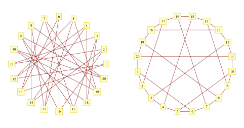
Figure 4: (L): The graph $H_{5,2}^{\prime}$. (R): The Desargues graph $H_{5,2}$. This is cospectral with $H_{5,2}^{\prime}$.

II.6 The Nauru graph and the Tutte-Coxeter graph

The Nauru graph, $N_{24}$, is the only cubic symmetric (arc-transitive) graph on $24$ vertices. It is bipartite, with spectrum $\left\{\pm 3,\pm 2^{[6]},\pm 1^{\left[3\right]},0^{\left[4\right]}\right\}$ and dia$\left(N_{24}\right)=4$. A brief parenthesis: the Foster census of cubic symmetric graphs highlights that a large portion of periodic cubic graph is symmetric con . Clearly, the two sets do not coincide. There are exactly seven different kind of entries in $U_{N_{24}}(t)$. This can be seen as a $2\times 2$ block matrix. The blocks $\left(1,1\right)$ and $\left(2,1\right)$ are below. The other blocks are just their rearrangements:

$$a_{1}$$

and

$$\begin{tabular}[c]{llllll|llllll}$a_{5}$&$a_{5}$&$a_{6}$&$a_{5}$&$a_{6}$&$a_{7}$&$a_{7}$&$a_{7}$&$a_{7}$&$a_{7}$&$a_{6}$&$a_{7}$\\ $a_{5}$&$a_{6}$&$a_{5}$&$a_{7}$&$a_{7}$&$a_{5}$&$a_{6}$&$a_{7}$&$a_{7}$&$a_{7}$&$a_{7}$&$a_{6}$\\ $a_{6}$&$a_{7}$&$a_{7}$&$a_{7}$&$a_{5}$&$a_{5}$&$a_{7}$&$a_{6}$&$a_{6}$&$a_{7}$&$a_{7}$&$a_{5}$\\ $a_{7}$&$a_{5}$&$a_{7}$&$a_{6}$&$a_{5}$&$a_{6}$&$a_{7}$&$a_{5}$&$a_{7}$&$a_{6}$&$a_{7}$&$a_{7}$\\ $a_{7}$&$a_{7}$&$a_{6}$&$a_{7}$&$a_{6}$&$a_{5}$&$a_{5}$&$a_{5}$&$a_{7}$&$a_{7}$&$a_{6}$&$a_{7}$\\ $a_{7}$&$a_{7}$&$a_{5}$&$a_{6}$&$a_{7}$&$a_{6}$&$a_{5}$&$a_{7}$&$a_{5}$&$a_{6}$&$a_{7}$&$a_{7}$\\ \hline\cr$a_{6}$&$a_{5}$&$a_{5}$&$a_{7}$&$a_{7}$&$a_{7}$&$a_{7}$&$a_{6}$&$a_{6}$&$a_{5}$&$a_{7}$&$a_{7}$\\ $a_{7}$&$a_{7}$&$a_{6}$&$a_{7}$&$a_{6}$&$a_{7}$&$a_{7}$&$a_{7}$&$a_{5}$&$a_{5}$&$a_{6}$&$a_{5}$\\ $a_{7}$&$a_{5}$&$a_{5}$&$a_{7}$&$a_{7}$&$a_{7}$&$a_{6}$&$a_{5}$&$a_{7}$&$a_{5}$&$a_{5}$&$a_{6}$\\ $a_{5}$&$a_{6}$&$a_{5}$&$a_{6}$&$a_{7}$&$a_{6}$&$a_{7}$&$a_{7}$&$a_{7}$&$a_{6}$&$a_{5}$&$a_{5}$\\ $a_{6}$&$a_{7}$&$a_{5}$&$a_{5}$&$a_{7}$&$a_{7}$&$a_{5}$&$a_{6}$&$a_{6}$&$a_{7}$&$a_{5}$&$a_{7}$\\ $a_{7}$&$a_{7}$&$a_{5}$&$a_{5}$&$a_{5}$&$a_{7}$&$a_{6}$&$a_{7}$&$a_{5}$&$a_{7}$&$a_{7}$&$a_{6}$\end{tabular}\text{ },$$

where

$$a_{1}=\left(2+3\cos\left(t\right)+6\cos\left(2t\right)+\cos\left(3t\right)\right)/12,$$

are all the the different entries of the unitary matrix. From these functions, we can write

$$\max_{t\in\mathbb{R}^{+}}\left(\left|a_{j}\right|\right)=\left\{\begin{tabular}[c]{rr}$=1,$&$j=1$ and $t=2\pi;$\\ $\approx 1/2,$&$j=2$ and $t\approx\pi/4;$\\ $\approx 1/4,$&$j=3$ and $t\approx 6/5;$\\ $=2/3,$&$j=4$ and $t=\pi;$\\ $\approx 9/20,$&$j=5$ and $t\approx\pi/4;$\\ $=1/3,$&$j=6$ and $t=\pi/2;$\\ $\approx 3/10,$&$j=7$ and $t\approx 3\pi/4.$\end{tabular}\right.$$

The Tutte-Coxeter graph, $TC$, is illustrated in Fig. (5). This is the largest cubic graph giving a periodic dynamics. Its eigenvalues are $\left\{\pm 3,\pm 2^{\left[9\right]},0^{\left[10\right]}\right\}$. Let us describe how to write down the unitary matrix $U_{TC}$. In Fig. (5) we have ordered the vertices anticlockwise. Each even vertex is connected to odd vertices, and viz. As we have seen in previous examples, $TC$ is bipartite and its unitary has a block structure:

$$U_{TC}=\left[\begin{array}[c]{cc}A&B\\ B&C\end{array}\right].$$

The $ij$-th entry of the block $B$ is

$$\left[B\right]_{i,j}=\left\{\begin{tabular}[c]{rr}$-i\left(6\sin\left(2t\right)+\sin\left(3t\right)\right)/15,$&$\{i,j\}\in E(TC);$\\ $i\left(3\sin\left(2t\right)-2\sin\left(3t\right)\right)/30,$&$\{i,j\}\notin E(TC).$\end{tabular}\right.$$

The index $i$ runs over the odd numbers $1,3,...,29$; $j$ over the even ones, $2,4,...,30$. For any chosen $t$, none of the entries of $B$ can have unit absolute value. The blocks $A$ and $C$ have the same entries but rearranged:

$$\begin{tabular}[c]{lllllllllllllll}$a_{1}$&$a_{2}$&$a_{3}$&$a_{3}$&$a_{2}$&$a_{3}$&$a_{2}$&$a_{2}$&$a_{3}$&$a_{2}$&$a_{3}$&$a_{3}$&$a_{3}$&$a_{3}$&$a_{2}$\\ $a_{2}$&$a_{1}$&$a_{2}$&$a_{3}$&$a_{3}$&$a_{2}$&$a_{3}$&$a_{3}$&$a_{3}$&$a_{2}$&$a_{3}$&$a_{2}$&$a_{2}$&$a_{3}$&$a_{3}$\\ $a_{3}$&$a_{2}$&$a_{1}$&$a_{2}$&$a_{3}$&$a_{2}$&$a_{3}$&$a_{2}$&$a_{3}$&$a_{3}$&$a_{3}$&$a_{3}$&$a_{3}$&$a_{2}$&$a_{2}$\\ $a_{3}$&$a_{3}$&$a_{2}$&$a_{1}$&$a_{2}$&$a_{3}$&$a_{3}$&$a_{2}$&$a_{3}$&$a_{2}$&$a_{2}$&$a_{3}$&$a_{2}$&$a_{3}$&$a_{3}$\\ $a_{2}$&$a_{3}$&$a_{3}$&$a_{2}$&$a_{1}$&$a_{2}$&$a_{3}$&$a_{3}$&$a_{2}$&$a_{3}$&$a_{3}$&$a_{3}$&$a_{2}$&$a_{3}$&$a_{2}$\\ $a_{3}$&$a_{2}$&$a_{2}$&$a_{3}$&$a_{2}$&$a_{1}$&$a_{2}$&$a_{3}$&$a_{2}$&$a_{3}$&$a_{2}$&$a_{3}$&$a_{3}$&$a_{3}$&$a_{3}$\\ $a_{2}$&$a_{3}$&$a_{3}$&$a_{3}$&$a_{3}$&$a_{2}$&$a_{1}$&$a_{2}$&$a_{3}$&$a_{3}$&$a_{2}$&$a_{3}$&$a_{2}$&$a_{3}$&$a_{3}$\\ $a_{2}$&$a_{3}$&$a_{2}$&$a_{2}$&$a_{3}$&$a_{3}$&$a_{2}$&$a_{1}$&$a_{2}$&$a_{3}$&$a_{3}$&$a_{2}$&$a_{3}$&$a_{2}$&$a_{3}$\\ $a_{3}$&$a_{3}$&$a_{3}$&$a_{3}$&$a_{2}$&$a_{2}$&$a_{3}$&$a_{2}$&$a_{1}$&$a_{2}$&$a_{3}$&$a_{2}$&$a_{3}$&$a_{3}$&$a_{3}$\\ $a_{2}$&$a_{2}$&$a_{3}$&$a_{2}$&$a_{3}$&$a_{3}$&$a_{3}$&$a_{3}$&$a_{2}$&$a_{1}$&$a_{2}$&$a_{3}$&$a_{3}$&$a_{2}$&$a_{3}$\\ $a_{3}$&$a_{3}$&$a_{3}$&$a_{2}$&$a_{3}$&$a_{2}$&$a_{2}$&$a_{3}$&$a_{3}$&$a_{2}$&$a_{1}$&$a_{2}$&$a_{3}$&$a_{2}$&$a_{2}$\\ $a_{3}$&$a_{2}$&$a_{3}$&$a_{3}$&$a_{3}$&$a_{3}$&$a_{3}$&$a_{2}$&$a_{2}$&$a_{3}$&$a_{2}$&$a_{1}$&$a_{2}$&$a_{3}$&$a_{2}$\\ $a_{3}$&$a_{2}$&$a_{3}$&$a_{2}$&$a_{2}$&$a_{3}$&$a_{2}$&$a_{3}$&$a_{3}$&$a_{3}$&$a_{3}$&$a_{2}$&$a_{1}$&$a_{3}$&$a_{3}$\\ $a_{3}$&$a_{3}$&$a_{2}$&$a_{3}$&$a_{3}$&$a_{3}$&$a_{2}$&$a_{3}$&$a_{2}$&$a_{2}$&$a_{3}$&$a_{3}$&$a_{2}$&$a_{1}$&$a_{2}$\\ $a_{2}$&$a_{3}$&$a_{2}$&$a_{3}$&$a_{2}$&$a_{3}$&$a_{3}$&$a_{3}$&$a_{3}$&$a_{3}$&$a_{2}$&$a_{2}$&$a_{3}$&$a_{2}$&$a_{1}$\end{tabular},$$

where

$$a_{1}=\left(5+9\cos\left(2t\right)+\cos\left(3t\right)\right)/15,$$

and

$$\max_{t\in\mathbb{R}^{+}}\left(\left|a_{j}\right|\right)\left\{\begin{tabular}[c]{rr}$=1,$&$j=1$ and $t=2\pi;$\\ $\approx 3/10,$&$j=2$ and $t\approx 1/4;$\\ $\approx 13/50,$&$j=3$ and $t\approx 91/50.$\end{tabular}\right.$$

This last equation concludes the proof of the theorem. Notice that $U_{TC}(\pi)$ is $2\times 2$ block diagonal: the diagonal entries are $-13/15$; the off-diagonal ones $2/15$. The two blocks are Grover matrices. When $t=\pi/2$, all entries in the off-diagonal blocks are equal to $i/15$.

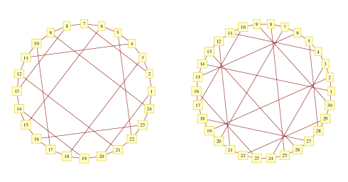
Figure 5: (L): The Nauru graph. (R): The Tutte-Coxeter graph. This is the largest periodic cubic graph. The Nauru graph and the Tutte-Coxeter graph do not have PST.

III Conclusions

We have shown that the 3-dimensional cube is the only periodic, connected cubic graph with PST. The proof is based on known results of graph theory and basic definitions of quantum dynamics on graphs. Our proof goes through the relevant cases, which can be interpreted as a systematical exploration of periodic quantum dynamics on cubic graphs. A necessary and sufficient condition for PST would give a shorter, more elegant proof. However, any method for the same task requires the different cases. There is a small plus in the approach adopted here: we have written down explicitly the unitary matrices that specify the dynamics. The matrices are potentially useful in further work. The well-known mathematical scenario of state transfer together with various facts observed in this paper suggest some reflections. These may be worth a mention.

III.1 Extremality

The literature on interconnection networks for telecommunications, parallel computers and distributed systems contain many optimization scenarios dealing with order/degree/diameter fe . The most famous one is perhaps the degree/diameter problem mil : given natural numbers $D$ and $\Delta$, find the largest possible number of vertices $n_{\Delta,D}$ in a graph of maximum degree $\Delta$ and diameter $\leq D$. The graphs achieving the upper bound are known as Moore graphs. Interestingly, in the setting of PST, the original problem was somehow the opposite one ch . In fact, the main point does not seek to maximize the number of vertices without compromising reachability, but to perform long distance communication, with a minimum of physical resources. The number of particles equals the order of the graph and it is therefore a resource. The order/distance problems for state transfer are then a new scenario, where graphs with extremal properties can be defined via some parameter associated to a dynamical process, instead of a topological condition. The landscape becomes even richer, if we consider more than a single excitation, and lift the analysis to the graph powers defined in godr . These considerations remind that the problem of identifying extremal graphs with respect to state transfer is still a mostly unexplored area of research.

III.2 A notion of persistency

As a generalization of the rule inducing a continuous-time random walk, the operator $U_{G}(t)=e^{-iA(G)t}$ has been subject of intense study (see mo and the references therein). In analogy with random walks, given the importance of these objects for constructing distributions, a principal direction has pointed uniform sampling. Additionally, still from the quantitative side, it is useful to deal with problems related to single vertices, or pairs of vertices, more than the entire graph. For example, an instance of relevant parameters is a quantum version of the hitting time. We would like to propose a notion that intends to quantify how the fidelity for state transfer between two vertices is constant in an interval, including small fluctuations. In the previous section, we have seen that half of the diagonal entries of $U_{C_{6}+K_{2}}(t)$ have the form $a_{1}=\left(2+\cos\left(t\right)+2\cos\left(2t\right)+\cos\left(3t\right)\right)/6$. When $t\in\{\pi/2,3\pi/2\}$, $a_{1}=0$. Roughly between $\pi/2$ and $3\pi/2$ there is a plateau: the value of the function is about $1/3$; it is exactly $1/3$, for $t=\pi$. Starting the process from some vertex $i$, if at time $t=\pi$ we sample from the distribution, we are going to obtain $i$ with probability $1/9$. This probability is not spicked, but fairly stable around $\pi$. Given a graph $G$, the $\epsilon$-persistency of a pair of vertices $i,j\in V(G)$ is the length of the longest interval $T\subset[0,2\pi]$ such that there exists a value $k$ for which $k-\epsilon<\left|[U_{G}(t)]_{i,j}\right|<k+\epsilon$, with $\epsilon\geq 0$, for every $t\in T$. By looking at all vertices, one could define the maximum persistency or the average persistency, if extending the definition in the obvious ways. A process with higher persistency requires less clock precision for sampling. A first sight reason for giving attention to persistency could arise from a connection with energy transfer problems ca . Let us add an additional remark. Decoherence has been shown to behave as a natural smoothing mechanism on probability amplitudes ke . Because of this fact, does decoherence increase persistency? With a similar scope but a on a different line, is the presence of decoherence compatible with PST at all?

III.3 Discrete probability transfer

The evolution governed by the Hamiltonian $H_{XY}(G)$ is driven by the exponentially smaller $U_{G}(t)$, when taking into account a single excitation only. While $A(G)$ faithfully represents $G$, the matrix $U_{G}(t)$ does not preserve its topological structure. In other words, $[U_{G}(t)]_{i,j}\neq 0$ does not imply $[A(G)]_{i,j}=1$. A discrete evolution on $G$ could be defined (in some cases ss ) by a unitary $W_{G}$, with $[W_{G}]_{i,j}\neq 0$ if and only if $[A(G)]_{i,j}=1$. Such a process does not describe the transfer of a single excitation, but it only allows to create a probability distribution supported by $V(G)$. The process is discrete and it follows the iteration $W_{G}W_{G}^{t-1}\longmapsto W_{G}^{t}$. If there is $t\in\mathbb{N}$ such that $\left|\langle j|W_{G}^{t}|i\rangle\right|=1$ then we have perfect probability transfer from vertex $i$ to vertex $j$. Unless we make use of some kind of lifting amb (e.g., the introduction of extra degrees of freedom), this is the closest analogue to the continuous object $U_{G}(t)$, even if this one does not always exist. For example, we can construct on $K_{4}$ the unitary below:

$$W_{K_{4}}=\left[\begin{array}[c]{cccc}0&-1&1&1\\ 1&0&-1&1\\ 1&-1&0&-1\\ 1&1&1&0\end{array}\right].$$

However, it is simple to observe that each power of $W_{K_{4}}$ has one of the two zero-patterns

$$\left[\begin{array}[c]{cccc}0&\ast&\ast&\ast\\ \ast&0&\ast&\ast\\ \ast&\ast&0&\ast\\ \ast&\ast&\ast&0\end{array}\right]$$ or

  

where $\ast$ denotes a generic nonzero entry. This is sufficient to show that $W_{K_{4}}$ does not give perfect probability transfer in $K_{4}$. In more complicated situations, the zero-patterns of matrix powers are not immediately available to imply a general statement. To verify that a graph $G$ does not enjoy the property, we should study the spectra of unitary matrices with the same zero-pattern of $W_{G}$. Since the problem involves both spectra, zero-pattern, and an optimization procedure, its flavour reminds of the matrix analysis questions approached in boy or various parametrizations coming from graph matrices hol . In our context, the use of semidefinite programming techniques does not seem immediately useful, because the matrices are not stochastic, but in fact unitary.

Acknowledgments. I am supported by a Newton International Fellowship. I am grateful to Matthew Russell for finding an important error in a previous version of the paper and an anonymous referee for valuable comments. This paper is dedicated to Anthony Sudbery in the occasion of his retirement.

References

References

(1)O. Ahmadi, N. Alon, I. F. Blake, I. E. Shparlinski, Graphs with
Integral Spectrum, Linear Algebra Appl., 430:1 (2009), pp. 547-552.
(2)A. Ambainis, Quantum Random Walks – New Method for Designing
Quantum Algorithms, SOFSEM 2008: Theory and Practice of Computer
Science,LNCS, 4910 (2008).
(3)R. J. Angeles-Canul, R. Norton, M. Opperman, C. Paribello, M.
Russell, C. Tamon, On quantum perfect state transfer in weighted join graphs,
Preprint 2009. arXiv:0909.0431v1 [quant-ph]
(4)K. Audenaert, C. D. Godsil, G. F. Royle, T. Rudolph, Symmetric
squares of graphs, J. Comb. Theory, Ser. B97(1): 74-90
(2007). arXiv:math/0507251v1 [math.CO]
(5)K. Balińska, D. M. Cvetković, Z. Radosavljević, S.
Simić, D. Stevanović, A survey on integral graphs, Univ.
Beograd, Publ. Elektrotehn. Fak., Ser. Mat. 13 (2002), 42-65.
(6)A. Bernasconi, C. Godsil, S. Severini, Quantum networks on
cubelike graphs, Phys. Rev. A78, 052320 (2008).
arXiv:0808.0510v1 [quant-ph]
(7)R. Bluhm, A. Kostelecky, J. Porter, B. Tudose, Revivals of
Quantum Wave Packets, COLBY 97-09, IUHET 372, September 1997, arXiv:quant-ph/9711061v1
(8)S. Boyd, P. Diaconis, J. Sun, and L. Xiao, Fastest mixing Markov
chain on a path, Amer. Math. Monthly, 113 (2006), pp. 70–74.
(9)S. Bose, Quantum Communication through Spin Chain Dynamics: an
Introductory Overview, Contemporary Physics, Vol. 48 (1), pp.
13-30, 2007. arXiv:0802.1224v1 [cond-mat.other]
(10)S. Bose, A. Casaccino, S. Mancini, S. Severini, Communication
in XYZ All-to-All Quantum Networks with a Missing Link, Int. J. Quantum
Info., 7:3 (2009). arXiv:0808.0748v1 [quant-ph]
(11)F. C. Bussemaker and D. M. Cvetković, There are exactly 13
connected, cubic, integral graphs, Univ. Beograd, Publ. Elektrotehn.
Fak., Ser. Mat. Fiz., Nos. 544-576 (1976), 43-48.
(12)F. Caruso, A. W. Chin, A. Datta, S. F. Huelga, and M. B. Plenio,
Highly efficient energy excitation transfer in light-harvesting complexes: The
fundamental role of noise-assisted transport, J. Chem. Phys.,
131 (10):105106, 2009. arXiv:0901.4454v2 [quant-ph]
(13)M. Christandl, N. Datta, A. Ekert and A. J. Landahl, Perfect
state transfer in quantum spin networks, Phys. Rev. Lett.92,
(2004), 187902. arXiv:quant-ph/0309131v2
(14)M. Conder, P. Dobcsányi, Trivalent Symmetric Graphs Up to
768 Vertices, J. Combin. Math. Combin. Comput.40,
41-63, 2002.
(15)D. M. Cvetković, M. Doob, H. Sachs, Spectra of graphs
– Theory and application. Deutscher Verlag der Wissenschaften – Academic
Press, Berlin-New Tork, 1980.
(18)H. van der Holst, L. Lovász, and A. Schrijver, The Colin de
Verdiere graph parameter, Graph theory and combinatorial biology
(Balatonlelle, 1996), Bolyai Soc. Math. Stud, 7, Janos Bolya
math. Soc. Budapest (1999), 29-85.
(19)V. Kendon, Decoherence in quantum walks - a review, Math.
Struct. in Comp. Sci17(6) pp. 1169-1220 (2006). arXiv:quant-ph/0606016v3
(20)M. Miller, J. Širáň, Moore graphs and beyond: A
survery of the degree/diameter problem, Elec. J. Comb. (2005), #DS14.
(21)M. Mosca, Quantum Algorithms, Springer Encyclopedia of
Complexity and Systems Science (Springer, New York, 2009). arXiv:0808.0369v1 [quant-ph]
(22)O. Ore, Theory of graphs, American Mathematical Society, 1962.
(23)M. Russell, Personal communication, January 2010.
(24)A. J. Schwenk, Exactly thirteen connected cubic graphs have
integral spectra. Proc. Int. Graph Thory Conf.at Kalamazoo, May
1976, (Y. Alavi and D. Licks, Eds.) Springer-Verlag.
(25)S. Severini, On the digraph of a unitary matrix, SIMAX,
SIAM J. Matrix Anal. Appl., 25, 1 (2003), pp. 295-300. arxiv:math.CO/0205187.
(26)W. Tadej, K. Życzkowski, A concise guide to complex Hamadard
matrices, Open Syst. Inf. Dyn. 13, 133-177 (2006). arXiv:quant-ph/0512154v2