Surface losses and self-pumping effects in a long
Josephson junction — a semi-analytical approach

Abstract

The flux-flow dynamics in a long Josephson junction is studied both analytically and numerically. A realistic model of the junction is considered by taking into account a nonuniform current distribution, surface losses and self-pumping effects. An approximate analytical solution of the modified sine-Gordon equation is derived in the form of a unidirectional dense fluxon train accompanied by two oppositely directed plasma waves. Next, some macroscopic time-averaged quantities are calculated making possible to evaluate the current-voltage characteristic of the junction. The results obtained by the present method are compared with direct numerical simulations both for the current-voltage characteristics and for the loss factor modulated spatially due to the self-pumping. The comparison shows very good agreement for typical junction parameters but indicates also some limitations of the method.

I Introduction

In recent years the flux-flow (FF) dynamics in a long Josephson junction has attracted considerable attention in view of possible applications in superconducting mm-wave electronics jpn ; kosh1 ; kosh2 ; kosh3 . The FF mode appears in a junction immersed in a sufficiently large external magnetic field and can be described briefly as a unidirectional viscous flow of a dense train of fluxons (magnetic flux quanta).

Recently, the FF oscillators have found various applications, e.g. in mm-wave integrated receivers kosh3 ; kosh4 ; kosh5 ; kosh6 , however some important parameters, such as the radiation line-width are still not satisfactory. Therefore, there is still a need for more adequate description of a real Josephson junction operating in the FF mode, by taking into account some additional factors which may affect the current-voltage ($I$-$V$) characteristic of the junction and change its working conditions.

In the majority of papers dealing with long Josephson junctions (see e.g. Refs. sml, ; lom, ; km, ; cir, ; ss1, ; mj1, ; mj2, ) a simplified version of the the sine-Gordon (sG) equation is considered, usually neglecting surface losses and assuming uniform distribution of the bias current density. Only recently, a few papers have been published pank1 ; pank2 ; pank3 ; mj3 taking into account a nonuniform bias current distribution and its influence on the junction behavior. Moreover, in Refs. pank2, ; pank3, a realistic model of the FF oscillator has been investigated both experimentally and numerically, including general boundary conditions, nonuniform bias current profile, surface losses as well as self-pumping effects tf related to additional tunneling of quasiparticles due to the Josephson radiation.

The aim of the present paper is to present an analytical approach to the modified sG equation, which takes into account:(i) nonuniform current distribution, (ii) surface losses, and (iii) spatial modulation of the loss factor resulting from the self-pumping effect. Contrary to Ref. pank2, we assume standard open-circuit boundary conditions to make the influence of various effects more pronounced. Nevertheless, the present analysis can be easily extended to include also more general boundary conditions.

In the particular case of uniform current distribution, the present method makes it possible to obtain fully analytical closed-form expressions describing both the superconducting phase within the junction and the $I$-$V$ characteristic. Such a solution can be regarded as the first-order approximation which appears sufficiently accurate for some moderate junction parameters. However, in the general case, particularly for very long and weakly damped junctions, such an analytical approximation is only the first step in an iterative procedure, which has to be performed numerically. Thus, in spite of analytical expressions describing the superconducting phase within the junction, the present approach has been named “semi-analytical”.

The paper is organized as follows. In Sec. II we formulate the problem, i.e. we present a generalized sG equation subject to open-circuit boundary conditions at the junction ends. Approximate analytical solutions to the sG equation are discussed in Sec. III. We start with a linearized (small-amplitude) solution and apply appropriate boundary conditions. Next, some large-amplitude corrections are introduced, we discuss also possible self-pumping effects and their influence on the $I$-$V$ characteristic. In Sec. IV analytical results are compared with direct numerical simulations. In particular, we discuss the influence of surface losses both for junctions of moderate length and for more realistic structures, such as very long junctions with small damping and strongly nonuniform current distribution. Sec. V contains concluding remarks, we indicate also possible extensions of the method by taking into account more general boundary conditions.

II Formulation of the problem

Fluxon dynamics in a long Josephson junction is usually described by the following modified sG equation sml ; lom ; km ; cir ; ss1 :

$$\phi_{xx}-\phi_{tt}-\alpha\phi_{t}=\sin\phi-\gamma,$$ (1)

where $\phi$ denote the quantum phase difference across the barrier, $\alpha$ is the loss factor, and $\gamma$ is the bias current density. The spatial coordinate $x$ has been normalized to the Josephson penetration depth $\lambda_{J}$ and the time coordinate $t$ to the inverse plasma frequency $\omega_{0}^{-1}$, where $\lambda_{J}=(\hbar/2\mu_{0}edj_{c})^{1/2}$, $\omega_{0}=(2ej_{c}/\hbar C)^{1/2}$, $j_{c}$ is the critical current density and $C$ denotes the junction capacitance per unit area.

However, to describe more adequately a real physical situation, one can consider a more general form pank2 ; pank3 :

$$\phi_{xx}-\phi_{tt}-\alpha(x)\phi_{t}+\beta\phi_{xxt}=\sin\phi-\gamma(x),$$ (2)

where $\beta$ denotes the surface loss parameter and we assume both $\alpha$ and $\gamma$ to be $x$-dependent, taking into account both a spatial modulation of the loss factor due to the self-pumping and a nonuniform distribution of the current density along the junction.

For the overlap geometry one can neglect the self-fields and assume simple open-circuit boundary conditions lom :

$$\phi_{x}(\pm L/2)+\beta\phi_{xt}(\pm L/2)=h,$$ (3)

where $h=H_{\rm ext}/j_{c}\lambda_{J}$, $H_{\rm ext}$ denotes the external magnetic field, and $L\gg 1$ is the normalized junction length.

Following Refs. ss1, ; cir, ; mj1, ; mj2, ; mj3, we look for an approximate solution in a form of a dense fluxon train traveling on a rotating background. Thus, a linearized solution of Eq. (2) can be written as

$$\phi=\phi_{0}+\psi,$$ (4)

where $\phi_{0}=\theta(x)+\Omega t$ is the background term (linear in time) and $\psi$ denotes a quasi-linear term (usually small) representing the motion of fluxons and plasma waves within the junction.

Substituting Eq. (4) into Eq. (2) we find

$$\theta_{xx}+\psi_{xx}-\psi_{tt}-\alpha\Omega-\alpha\psi_{t}+\beta\psi_{xxt}=\sin(\phi_{0}+\psi)-\gamma.$$ (5)

We are interested in a steady-state, time periodic solution, thus the background frequency $\Omega$ should be equal to the fundamental frequency of the oscillating term $\psi$. Both experimental data and numerical simulations show that the output signal of a real FF oscillator is nearly sinusoidal jpn ; pank1 . Thus, it is reasonable to assume the time-dependence of the term $\psi$ to be harmonic in $\Omega t$, and neglect any higher harmonics generated by the nonlinear term $\sin(\phi_{0}+\psi)$. Consequently, Eq. (5) can be split into a time-independent part and a part oscillating with frequency $\Omega$, while the boundary conditions (3) can be written separately for $\theta(x)$ and $\psi(x,t)$:

$$\theta_{x}(\pm L/2)=h,$$ (6)

$$\psi_{x}(\pm L/2)+\beta\psi_{xt}(\pm L/2)=0.$$ (7)

III Approximate analytical solution

The method for solving Eq. (5) with the boundary conditions (6) and (7) is similar to that reported recently (see Ref. mj3, for details). Thus, below we discuss briefly only the main points of the analysis.

III.1 Time-independent equation

It can be easily shown that for $\psi$ oscillating with frequency $\Omega$, the nonlinear term $\sin(\phi_{0}+\psi)$ contributes also to the time-independent part of Eq. (5), and such a contribution yields, in fact, the first-order approximation of the $I$-$V$ characteristic of the junction. Thus, the time-independent equation can be written as:

$$\theta_{xx}=\alpha(x)\Omega+S(x)-\gamma(x),$$ (8)

where

$$S(x)=\langle\sin(\phi_{0}+\psi)\rangle_{T}=(1/T)\int_{0}^{T}\sin(\phi_{0}+\psi)dt,$$ (9)

and $T=2\pi/\Omega$.

Solving Eq. (8) for $\theta(x)$ we find

$$\theta=\int_{-L/2}^{x}\left[\int_{-L/2}^{\eta}[\alpha(\xi)\Omega+S(\xi)-\gamma(\xi)]d\xi\right]d\eta+C_{1}x+C_{2}.$$ (10)

Without loss of generality $C_{2}$ can be set to zero while from the boundary condition (6) we find $C_{1}=h$ and

$$\gamma_{0}=\alpha_{0}\Omega+\frac{1}{L}\int_{-L/2}^{L/2}S(x)dx,$$ (11)

where $\gamma_{0}$, $\alpha_{0}$ denote the averaged current density and loss factor, respectively:

$$\gamma_{0}=\frac{1}{L}\int_{-L/2}^{L/2}\gamma(x)dx,\qquad\alpha_{0}=\frac{1}{L}\int_{-L/2}^{L/2}\alpha(x)dx.$$ (12)

It follows from the relation (4) that the time-averaged value of $\phi_{t}$, (being proportional to the constant voltage) is equal to the frequency $\Omega$. Thus, the expression (11) can be regarded as the current-voltage ($I$-$V$) characteristic of the Josephson junction. One can see that the total current density $\gamma_{0}$ consists of a linear (Ohmic) part and a nonlinear contribution related to the Josephson current.

III.2 Time-dependent equation

For $\psi$ sufficiently small we can write

$$\sin(\phi_{0}+\psi)\simeq\sin\phi_{0}+\psi\cos\phi_{0}.$$ (13)

Noting that the term $\psi\cos\phi_{0}$ gives no contribution of frequency $\Omega$ and collecting all the time-dependent terms in Eq. (5) we find

$$\psi_{xx}-\psi_{tt}-\alpha(x)\psi_{t}+\beta\psi_{xxt}\simeq\sin\phi_{0}.$$ (14)

Since all the terms in Eq. (14) oscillate with the same frequency $\Omega$, it is convenient to use a complex notation mj2 ; mj3

$$\psi(x,t)={\rm Im}\left[\widehat{\psi}(x)e^{i\Omega t}\right],\qquad\sin\phi_{0}={\rm Im}\left[e^{i(\theta+\Omega t)}\right],$$ (15)

and rewrite Eq. (14) as an ordinary differential equation

$$(1+i\Omega\beta)\widehat{\psi}_{xx}+(\Omega^{2}-i\alpha(x)\Omega)\widehat{\psi}=e^{i\theta},$$ (16)

or

$$\widehat{\psi}_{xx}+\delta^{2}\widehat{\psi}=e^{i\theta}/P,$$ (17)

where $P=1+i\Omega\beta$, $\delta^{2}=(\Omega^{2}-i\alpha(x)\Omega)/P$.

The general approximate solution of Eq. (17) can be written in a WKB-like form mf

$$\widehat{\psi}(x) = \frac{1}{2iP\sqrt{\delta}}\left[e^{if(x)}F^{-}(x)-e^{-if(x)}F^{+}(x)\right]$$ (18)

$$+A\frac{e^{if(x)}}{\sqrt{\delta}}+B\frac{e^{-if(x)}}{\sqrt{\delta}},$$

where

$$F^{\pm}(x)=\int_{-L/2}^{x}\frac{e^{i(\theta(\xi)\pm f(\xi))}d\xi}{\sqrt{\delta}},\quad f(x)=\int_{-L/2}^{x}\delta(\xi)d\xi.$$ (19)

The term in square brackets in Eq. (18) corresponds to a dense fluxon train moving unidirectionally along the junction, while the last two terms describe two plasma waves propagating in opposite directions.

Using the complex formalism the boundary condition (7) can be rewritten as

$$\widehat{\psi}_{x}(\pm L/2)+i\Omega\beta\widehat{\psi}_{x}(\pm L/2)=0\ \Longrightarrow\ \widehat{\psi}_{x}(\pm L/2)=0.$$ (20)

Thus, using Eqs. (18) and (20) one can determine the integration constants $A$ and $B$ to be

$$A=B=\frac{e^{i\delta_{0}L}F^{-}(L/2)+e^{-i\delta_{0}L}F^{+}(L/2)}{4P\sin\delta_{0}L},$$ (21)

where

$$\delta_{0}=\frac{1}{L}\int_{-L/2}^{L/2}\delta(x)dx.$$ (22)

It should be mentioned here that the solutions for $\theta$ and $\widehat{\psi}$ (Eqs. (10) and (18), respectively) are not given explicitly but rather form a system of coupled equations. Fortunately, this system can be easily solved by a method of consecutive iterations. Indeed, starting with $S(x)=0$ one can solve Eq. (10) for $\theta$ and next solve Eq. (18) for $\widehat{\psi}$. Substituting $\theta$ and $\widehat{\psi}$ into Eq. (9) we obtain a new approximation for $S(x)$ and consequently new approximations for $\theta$ and $\widehat{\psi}$.

It is clear from Eq. (11) that $S(x)=0$ corresponds simply to the Ohmic line $\gamma_{0}=\alpha_{0}\Omega$, while consecutive iterations yield a sequence of approximations for $S(x)$ describing the time-independent contribution from the Josephson current.

The rate of convergence of the iterative process depends strongly on the junction parameters. As shown in the next Section, for moderate values of $L$, $h$, and $\alpha_{0}$, the first iteration yields satisfactory results. However, for practical FF oscillators which are usually based on very long junctions, up to a few thousands of iterations are needed to obtain a self-consistent solution.

III.3 Analytical approximation

It is interesting that for the simplest, but widely used model of uniform bias current distribution ($\gamma(x)={\rm const}$), all the integrations can be performed analytically, leading to a compact and fully analytical expression for the $I$-$V$ characteristic.

Indeed, assuming the small-amplitude limit ($\widehat{\psi}\ll 1$) and ignoring self-pumping effects ($\alpha(x)=\rm const$), one can calculate the first-order approximation for Eq. (11). Following the steps outlined above we find $\theta(x)=hx$ and consequently

$$\widehat{\psi}(x) = -\frac{e^{ihx}}{P(h^{2}-\delta^{2})}+\frac{h\sin[(h+\delta)L/2]}{P(h^{2}-\delta^{2})\delta\sin\delta L}e^{i\delta x}$$ (23)

$$+\frac{h\sin[(h-\delta)L/2]}{P(h^{2}-\delta^{2})\delta\sin\delta L}e^{-i\delta x}$$

and

$$\gamma_{0}=\alpha_{0}\Omega+{\rm Im}\left[-\frac{1}{2P(h^{2}-\delta^{2})}+\frac{h^{2}(\cos\delta L-\cos hL)}{LP(h^{2}-\delta^{2})^{2}\delta\sin\delta L}\right],$$ (24)

where $P$ and $\delta$ have been defined in Eq. (17).

When the surface losses are neglected ($\beta=0$) the above simple expression is reduced to the solution derived earlier mj2 . Moreover, it can be shown that for $\beta=0$ the expression (24) is also equivalent to apparently different solutions derived independently in Refs. ss2, ; pank1, in a form of infinite series expansions.

III.4 Large-amplitude corrections

As follows from Eq. (11), the evaluation of $S(x)$ is crucial for the determination of $I$-$V$ characteristic. So far we have assumed $\psi\ll 1$ and used an approximation (13). However, for $\psi$ larger we should consider the exact relation

$$S(x)=\langle\sin\phi_{0}\cos\psi\rangle_{T}+\langle\cos\phi_{0}\sin\psi\rangle_{T}.$$ (25)

Since $\psi$ is an oscillatory function, one can use well-known relations as involving Bessel function. As shown in Ref. mj3, , the leading terms for $\cos\psi$ and $\sin\psi$ are given by

$$\cos\psi\simeq J_{0}(|\widehat{\psi}|),\qquad\sin\psi\simeq\frac{2J_{1}(|\widehat{\psi}|)}{|\widehat{\psi}|}\psi,$$ (26)

where $J_{0}$, $J_{1}$ denote the Bessel functions of order 0 and 1, respectively.

Using Eq. (26) we can find the time-independent contribution $S(x)$ to be mj3

$$S(x)=\frac{J_{1}(|\widehat{\psi}|)}{|\widehat{\psi}|}{\rm Im}\left[\widehat{\psi}e^{-i\theta}\right].$$ (27)

Accordingly, the right-hand sides of Eqs. (14) and (16) should be replaced by $\sin\phi_{0}\cos\psi$ and $J_{0}(|\widehat{\psi}|)e^{i\theta}$, respectively.

III.5 Self-pumping effects

According to Refs. pank2, ; pank3, , the total current density due to the quasi-particle tunneling is given by

$$\gamma_{\rm eff}=\sum_{-\infty}^{\infty}J_{n}^{2}\left(ev_{\rm ac}/\hbar\omega\right)\gamma_{\rm dc}(v_{\rm dc}+n\hbar\omega/e),$$ (28)

where $J_{n}$ is the Bessel functions of order $n$, $\gamma_{\rm dc}$ denotes the unpumped $I$-$V$ dependence, and the total voltage applied to the junction can be separated into a constant ($v_{\rm dc}$) part and and an oscillatory part of amplitude $v_{\rm ac}$ and frequency $\omega$.

Using the Josephson relation bp $v_{\rm dc}=\hbar\omega/2e$ and coming back to our dimensionless notation we find $v_{\rm dc}=\Omega$, $v_{\rm ac}=|\widehat{\psi}|\Omega$ and

$$\gamma_{\rm eff}=\sum_{-\infty}^{\infty}J_{n}^{2}\left(|\widehat{\psi}|/2\right)\gamma_{\rm dc}\left[\Omega(1+2n)\right].$$ (29)

For small arguments $z=|\widehat{\psi}|/2\ll 1$ the infinite expansion (29) can be truncated to include only quadratic terms in $z$:

$$\gamma_{\rm eff}=\gamma_{\rm dc}(\Omega)+\frac{z^{2}}{4}\left[\gamma_{\rm dc}(-\Omega)-2\gamma_{\rm dc}(\Omega)+\gamma_{\rm dc}(3\Omega)\right].$$ (30)

As an unpumped $I$-$V$ characteristic we can take the nonlinear resistive model lik

$$\gamma_{\rm dc}(\Omega)=\alpha_{0}\Omega\left\{b\frac{(\Omega/\Omega_{g})^{n}}{[(\Omega/\Omega_{g})^{n}+1]}+1\right\},$$ (31)

where $n\gg 1$, $\Omega_{g}$ denotes the normalized gap voltage and $b=R_{j}/R_{n}$ is the ratio of normal-state resistances below and above $\Omega_{g}$.

For $n\rightarrow\infty$ the highly nonlinear continuous dependence (31) tends to a simple discontinuous linear form which will be used in further calculations:

$$\gamma_{\rm dc}=\left\{\begin{array}[]{l}\alpha_{0}\Omega\\ \alpha_{0}\Omega(b+1)\end{array}\right.\quad\mbox{for}\quad\begin{array}[]{l}\Omega<\Omega_{g},\\ \Omega>\Omega_{g}.\end{array}$$ (32)

It is clear that $\gamma_{\rm eff}$ is $x$-dependent due to the self-pumping via $\widehat{\psi}(x)$, thus we can define an effective damping factor $\alpha_{\rm eff}(x)=\gamma_{\rm eff}(x)/\Omega$ and compute it self-consistently by starting with $\alpha_{\rm eff}=\alpha_{0}$, calculating $\widehat{\psi}$, substituting into Eq. (29), evaluating a new approximation for $\alpha_{\rm eff}(x)$, and so on.

IV Results and discussion

In this section we compare analytical results derived above with numerical simulations obtained by the finite-difference implicit scheme dodd . The $I$-$V$ characteristic is given by Eq. (11), while $S(x)$ follows from the self-consistent solutions of Eqs. (10) and (18). To illustrate the influence of surface losses we consider first the simplest case $\gamma(x)={\rm const}$ where the $I$-$V$ dependence can be expressed in a closed form (24).

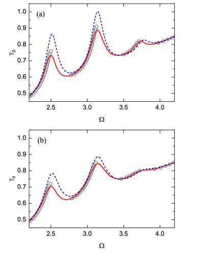
Figure 1: (Color online) Current-voltage characteristic calculated analytically (solid line) and numerically (open circles) for $\gamma(x)=\rm const$, $L=5$, $h=3$, $\alpha_{0}=0.2$: (a) $\beta=0$, (b) $\beta=0.01$. The dashed line shows the first-order approximation (24).

Fig. 1 shows the central part of the $I$-$V$ characteristic for a junction of moderate length $L=5$. The remaining parameters ($\alpha_{0}=0.2$, $h=3$) are similar to those assumed in Ref. pank1, . Open circles denote the results of numerical simulations for a discrete set of $\gamma_{0}$ points. The dashed line denotes the analytical solution (24) while the solid line follows from the self-consistent solutions (10) and (18) obtained by consecutive iterations for $\theta$ and $\widehat{\psi}$. Fig. 1(a) shows the case $\beta=0$ (no surface losses) and in Fig. 1(b) we assume $\beta=0.01$. Similar results for $h=5$ are presented in Fig. 2(a),(b).

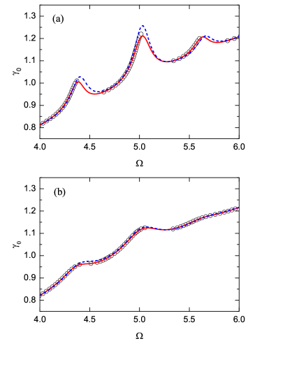
Figure 2: (Color online) the same as in Fig. 1 but for $h=5$.

One can see that the $I$-$V$ dependence departs from the Ohmic line $\gamma_{0}=\alpha_{0}\Omega$ in the region of $\Omega\simeq h$, forming the main FF step modulated by a series of Fiske steps with voltage spacing $\Delta\Omega\simeq\pi/L$. Analytical approximations are continuous and consist of a series of resonances while numerical results show typical hysteretic behavior and we observe only the segments of positive slope.

It is clear that the presence of even very small surface losses changes significantly the $I$-$V$ dependence. Generally, the steps (resonances) become smaller and this effect is more pronounced for larger values of the external field $h$. Such a result can be easily explained if we recall that the main FF step and accompanying Fiske steps are visible in the region $\Omega\simeq h$ and the surface loss factor enters the formalism via $P=1+i\Omega\beta$. In other words, for higher external magnetic field the influence of surface losses is stronger and the $I$-$V$ characteristic becomes more smooth. The influence of surface losses is clearly visible in experimental results pank2 ; pank3 , where the Fiske steps gradually disappear as the external magnetic field is getting stronger.

Comparing analytical and numerical results shown in Figs. 1 and 2 one can see that the fully analytical solution (dashed line) is fairly accurate. On the other hand, the self-consistent solution (solid line) reproduces very accurately all the details of the numerical solution.

As the next example, let us consider a more realistic case of a very long junction with small damping. Following Ref. pank3, we choose $L=40$, $\alpha_{0}=0.033$, $\beta=0.035$, and a slightly asymmetric current profile $\gamma(x)$ depicted in Fig. 3. The bias electrode ($x_{1}\leq x\leq x_{2}$) is shorter than the total junction length. Consequently, the current distribution is assumed parabolic for $x_{1}\leq x\leq x_{2}$, and exponential in the unbiased tails ($x\leq x_{1}$, $x\geq x_{2}$).

Figure 3: Normalized bias current distribution similar to that assumed in Ref. pank3, . $L=40$, $x_{1}=-9$, $x_{2}=5.5$.

Contrary to the previous example, now we cannot use the analytical approximation (24). First, the current distribution is $x$-dependent, what means that $\theta(x)$ departs from a simple linear dependence $\theta(x)=hx$, and relevant integrals cannot be calculated analytically. Second, it appears (even for a uniform current profile) that the first-order approximation is not accurate enough for very long junctions, and consecutive iterations are necessary to obtain a self-consistent solution.

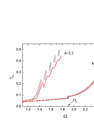
Figure 4: (Color online) Current-voltage characteristic calculated analytically (solid line) and numerically (open circles) for two values of the external magnetic field: $h=2.5$ and $h=3.5$. The current profile is shown in Fig. 3 and the remaining junction parameters are: $L=40$, $\alpha_{0}=0.033$, $\beta=0.035$.

Fig. 4 shows the $I$-$V$ characteristics calculated for junction parameters specified above and for two values of the external magnetic field $h=2.5$ and $h=3.5$. As before, open circles correspond to numerical simulations while the solid line represents a self-consistent solution. One can see that the agreement between numerical and analytical results is rather poor for $h=2.5$. To explain this discrepancy we should recall the main assumption (see Sec. II) that Eq. (5) can be separated into a time-independent part and a part sinusoidal in $\Omega t$ while neglecting higher-order harmonics. The Fourier analysis shows, however, that the anharmonic contribution to $\psi(t)$ is rather large for $h=2.5$. E.g. for $\gamma_{0}=0.3$ we find the content of the second harmonic to be about 35%. Physically, it means that the fluxon train is not sufficiently dense for $h=2.5$ and its time-dependence although periodic is not strictly sinusoidal.

Contrary to the case $h=2.5$, for $h=3.5$ we observe excellent agreement between numerical and analytical data. Now the $I$-$V$ characteristic is smooth and the Fiske steps disappeared completely as a combined result of surface losses and self-pumping effects. The Fourier analysis of $\psi(t)$ shows now that the anharmonicity diminishes rather quickly with increasing $h$ and for $h=3.5$ we observe only about 10% of the second harmonic.

Another interesting feature which is visible for $h=3.5$ is an additional small step at $\Omega_{b}=1.9$. Such a step appears in experimental results pank3 ; kosh7 and can be attributed to the self-pumping effect described in Subsection III.E. As shown in Ref. kosh7, , the position of the current step follows from a simple relation $\Omega_{b}=\Omega_{g}/3$, where $\Omega_{g}$ denotes the gap voltage. Assuming typical junction parameters kosh7 we find a normalized dimensionless gap voltage $\Omega_{g}=5.7$, hence $\Omega_{b}=1.9$.

It is interesting that the value of $\Omega_{b}$ can also be deduced directly form Eq. (30). Indeed, noting that $\gamma_{\rm dc}(-\Omega)=-\gamma_{\rm dc}(\Omega)$ one can see the quadratic term in Eq. (30) to vanish, provided $\gamma_{\rm dc}(\Omega)$ is a linear function. However, for a nonlinearity starting at $\Omega=\Omega_{g}$ we find $\gamma_{\rm dc}(3\Omega)\neq 3\gamma_{\rm dc}(\Omega)$, thus a nonzero contribution to $\gamma_{\rm eff}$ appears at $3\Omega=\Omega_{g}$, giving rise to a step at $\Omega_{b}=\Omega_{g}/3$.

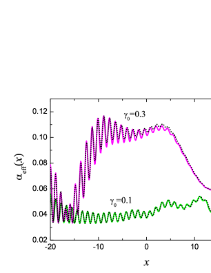
Figure 5: (Color online) Spatial distribution of $\alpha_{\rm eff}(x)$ calculated analytically (solid line) and numerically (dotted line) for $h=3.5$ and two values of the averaged current density $\gamma_{0}=0.1$ and $\gamma_{0}=0.3$. The remaining junction parameters are the same as in Fig. 4.

As shown in Subsection III.E, an effective loss factor $\alpha_{\rm eff}(x)$ is spatially modulated due to the self-pumping, and its average value becomes significantly larger than $\alpha_{0}$. Fig. 5 shows the spatial distribution of $\alpha_{\rm eff}$ plotted for $\gamma_{0}=0.1$ and $\gamma_{0}=0.3$. The junction parameters are assumed as before. i.e. $L=40$, $h=3.5$, $\alpha_{0}=0.033$, $\beta=0.035$. Now the dotted lines correspond to numerical simulations and the solid lines denote self-consistent (analytical) solutions. One can see that the agreement is excellent, the self-consistent solution following closely all the details of the numerical simulations, taken here as a reference.

It is clear that $\alpha_{\rm eff}$ generally grows with increasing value of $\gamma_{0}$. E.g. for $\gamma_{0}=0.3$ we obtain an averaged value of $\alpha_{\rm eff}(x)$ about three times larger than the “unpumped” value $\alpha_{0}$. Such an effect together with surface losses makes the $I$-$V$ curve smooth, damping effectively the Fiske steps.

V Conclusions

In this paper a semi-analytical approach has been suggested, making possible to solve a modified sG equation (2) with both surface losses and self-pumping effects taken into account. The solution, as given by Eqs. (4), (10), and (18), consists of a rotating background and a unidirectional fluxon train accompanied by two plasma waves traveling in opposite directions with the velocity close to the critical value $\Omega/\delta_{0}\simeq\pm 1$. Having obtained an analytical solution to Eq. (2) one can determine some macroscopic, directly measurable quantities, such as the constant bias current and constant voltage, making possible to calculate the $I$-$V$ characteristic (11) of the junction.

For the uniform current density distribution ($\gamma(x)=\rm const$) it has been shown that the relevant expressions for $\theta(x)$, $\widehat{\psi}(x)$, and consequently the $I$-$V$ dependence can be obtained in a closed fully analytical form (24). As follows from Figs. 1 and 2, such an approximation is fairly accurate for moderate junction parameters. In general, however, practical FF oscillators are based on very long junctions with strongly nonuniform current profile. In such a case an analytical approximation (24) appears insufficient and one should look for a self-consistent solution of Eqs. (10) and (18) which can be obtained by an iterative procedure.

As shown in Figs. 1,2,4 and 5, the self-consistent solutions and numerical simulations are generally in very good agreement. The only exception, where one can observe qualitative rather than quantitative agreement is the $I$-$V$ curve shown in Fig. 4 for $h=2.5$. As explained in the previous Section, the fluxon train is not dense enough for $h=2.5$ and consequently the time-dependent part of the solution is periodic but not strictly sinusoidal, violating the main assumption of the present approach.

Finally, it should be mentioned that the method presented here can be easily extended to include general, more realistic boundary conditions discussed in Refs. pank2, ; pank3, ; sor, . In the present paper, however, we intentionally assumed standard open-circuit boundary conditions (3), where the plasma waves could interfere after complete reflection at the boundaries, giving rise to clearly visible Fiske steps. This way, we were able to separate the influence of surface losses and self-pumping from that of boundary conditions, which (e.g. for a resistive load) can also affect the $I$-$V$ characteristic and make the physical mechanism discussed here less clear.

References

- (1) T. Nagatsuma, K. Enpuku, F. Irie, and K. Yoshida, J. Appl. Phys. 54, 3302 (1983); see also J. Appl. Phys. 56, 3284 (1984); 58, 441 (1985); 63, 1130 (1988).
- (2) V. P. Koshelets, A. V. Shchukin, S. V. Shitov, and L. V. Filippenko, IEEE Trans. Appl. Supercond. 3, 2524 (1993).
- (3) J. Mygind, V. P. Koshelets, A. V. Shchukin. S. V. Shitov, and I. L. Lapytskaya, IEEE Trans. Appl. Supercond. 5, 2951 (1995).
- (4) V. P. Koshelets and S. V. Shitov, Supercond. Sci. Technol. 13, R53 (2000).
- (5) V. P. Koshelets, S. V. Shitov, P. N. Dmitriev, A. B. Ermakov, L. V. Filippenko, V. V. Khodos, V. L. Vaks, A. M. Baryshev, P. R. Wesselius, and J. Mygind, Physica C 367, 249 (2002).
- (6) M. Y. Torgashin, V. P. Koshelets, P. N. Dmitriev, A. B. Ermakov, L. V. Filippenko, and P. A. Yagoubov, IEEE Trans. Appl. Supercond. 17, 379 (2007).
- (7) A. V. Khudchenko, V. P. Koshelets, P. N. Dmitriev, A. B. Ermakov, P. A. Yagoubov, and O. M. Pylypenko, Supercond. Sci. Technol. 22, 085012 (2009).
- (8) D. W. McLaughlin and A. C. Scott, Phys. Rev. A 18, 1652 (1978).
- (9) P. S. Lomdahl, J. Stat. Phys. 39, 551 (1985).
- (10) Yu. S. Kivshar and B. A. Malomed, Rev. Mod. Phys. 61, 763 (1978).
- (11) M. Cirillo, N. Grønbech-Jensen, M. R. Samuelsen, M. Salerno, and G. Verona Rinati, Phys. Rev. B 58, 12377 (1998).
- (12) M. Salerno and M. R. Samuelsen, Phys. Rev. B 61, 99 (2000).
- (13) M. Jaworski, Phys. Rev. B 60, 7484 (1999).
- (14) M. Jaworski, Supercond. Sci. Technol. 17, 327 (2004).
- (15) A. L. Pankratov, Phys. Rev. B 66, 134526 (2002).
- (16) A. S. Sobolev, A. L. Pankratov, and J. Mygind, Physica C 435, 112 (2006).
- (17) A. L. Pankratov, A. S. Sobolev, V. P. Koshelets, and J. Mygind, Phys. Rev. B 75, 184516 (2007).
- (18) M. Jaworski, Supercond. Sci. Technol. 21, 065016 (2008).
- (19) J. R. Tucker and M. J. Feldman, Rev. Mod. Phys. 57, 1055 (1985)
- (20) P. M. Morse and H. Feshbach, Methods of Theoretical Physics (McGraw-Hill, New York, 1953).
- (21) M. Salerno and M. R. Samuelsen, Phys. Rev. B 59, 14653 (1999).
- (22) M. Abramowitz and I.A. Stegun, Handbook of Mathematical Functions (Dover, New York, 1982).
- (23) A. Barone and G. Paterno, Physics and Applications of the Josephson Effect (Wiley, New York, 1982).
- (24) K. K. Likharev, Dynamics of Josephson Junctions and Circuits (Gordon and Breach, New York, 1986).
- (25) R. K. Dodd, J. C. Eilbeck, J. D. Gibbon, and H. C. Morris, Solitons and Nonlinear Wave Equations (Academic, London, 1982).
- (26) V. P. Koshelets, S. V. Shitov, A. V. Shchukin, L. V. Filippenko, J. Mygind, and A. V. Ustinov, Phys. Rev. B 56, 5572 (1997).
- (27) C. Soriano, G. Costabile, and R. D. Parmentier, Supercond. Sci. Technol. 9, 578 (1996).