Adaptive Wave Models for Option Pricing Evolution:
Nonlinear and Quantum Schrödinger Approaches

Vladimir G. Ivancevic
Defence Science & Technology Organisation, Australia
Abstract

Adaptive wave model for financial option pricing is proposed, as a high-complexity alternative to the standard Black–Scholes model. The new option-pricing model, representing a controlled Brownian motion, includes two wave-type approaches: nonlinear and quantum, both based on (adaptive form of) the Schrödinger equation. The nonlinear approach comes in two flavors: (i) for the case of constant volatility, it is defined by a single adaptive nonlinear Schrödinger (NLS) equation, while for the case of stochastic volatility, it is defined by an adaptive Manakov system of two coupled NLS equations. The linear quantum approach is defined in terms of de Broglie’s plane waves and free-particle Schrödinger equation. In this approach, financial variables have quantum-mechanical interpretation and satisfy the Heisenberg-type uncertainty relations. Both models are capable of successful fitting of the Black–Scholes data, as well as defining Greeks.

Keywords: Black–Scholes option pricing, adaptive nonlinear Schrödinger equation,
adaptive Manakov system, quantum-mechanical option pricing, market-heat potential

PACS: 89.65.Gh, 05.45.Yv, 03.65.Ge

1 Introduction

Recall that the celebrated Black–Scholes partial differential equation (PDE) describes the time–evolution of the market value of a stock option [1, 2]. Formally, for a function u=u(t,s)𝑢𝑢𝑡𝑠u=u(t,s) defined on the domain 0s<,0tTformulae-sequence0𝑠0𝑡𝑇0\leq s<\infty,~{}0\leq t\leq T and describing the market value of a stock option with the stock (asset) price s𝑠s, the Black–Scholes PDE can be written (using the physicist notation: zu=u/zsubscript𝑧𝑢𝑢𝑧\partial_{z}u=\partial u/\partial z) as a diffusion–type equation:

tu=12(σs)2ssurssu+ru,subscript𝑡𝑢12superscript𝜎𝑠2subscript𝑠𝑠𝑢𝑟𝑠subscript𝑠𝑢𝑟𝑢\partial_{t}u=-\frac{1}{2}(\sigma s)^{2}\,\partial_{ss}u-rs\,\partial_{s}u+ru, (1)

where σ>0𝜎0\sigma>0 is the standard deviation, or volatility of s𝑠s, r𝑟r is the short–term prevailing continuously–compounded risk–free interest rate, and T>0𝑇0T>0 is the time to maturity of the stock option. In this formulation it is assumed that the underlying (typically the stock) follows a geometric Brownian motion with ‘drift’ μ𝜇\mu and volatility σ𝜎\sigma, given by the stochastic differential equation (SDE) [3]

ds(t)=μs(t)dt+σs(t)dW(t),𝑑𝑠𝑡𝜇𝑠𝑡𝑑𝑡𝜎𝑠𝑡𝑑𝑊𝑡ds(t)=\mu s(t)dt+\sigma s(t)dW(t), (2)

where W𝑊W is the standard Wiener process. The Black-Scholes PDE (1) is usually derived from SDEs describing the geometric Brownian motion (2), with the stock-price solution given by:

s(t)=s(0)e(μ12σ2)t+σW(t).𝑠𝑡𝑠0superscripte𝜇12superscript𝜎2𝑡𝜎𝑊𝑡s(t)=s(0)\,\mathrm{e}^{(\mu-\frac{1}{2}\sigma^{2})t+\sigma W(t)}.

In mathematical finance, derivation is usually performed using Itô lemma [4] (assuming that the underlying asset obeys the Itô SDE), while in physics it is performed using Stratonovich interpretation [5, 6] (assuming that the underlying asset obeys the Stratonovich SDE [8]).

The Black-Sholes PDE (1) can be applied to a number of one-dimensional models of interpretations of prices given to u𝑢u, e.g., puts or calls, and to s𝑠s, e.g., stocks or futures, dividends, etc. The most important examples are European call and put options, defined by:

uCall(s,t)=s𝒩(d1)eTδk𝒩(d2)erT,subscript𝑢Call𝑠𝑡𝑠𝒩subscriptd1superscripte𝑇𝛿𝑘𝒩subscriptd2superscripte𝑟𝑇\displaystyle u_{\mathrm{Call}}(s,t)=s\,\mathcal{N}(\mathrm{d_{1}})\,\mathrm{e}^{-T\delta}-k\,\mathcal{N}(\mathrm{d_{2}})\,\mathrm{e}^{-rT}, (3)
uPut(s,t)=k𝒩(d2)erTs𝒩(d1)eTδ,subscript𝑢Put𝑠𝑡𝑘𝒩subscriptd2superscripte𝑟𝑇𝑠𝒩subscriptd1superscripte𝑇𝛿\displaystyle u_{\mathrm{Put}}(s,t)=k\,\mathcal{N}(-\mathrm{d_{2}})\,\mathrm{e}^{-rT}-s\,\mathcal{N}(-\mathrm{d_{1}})\,\mathrm{e}^{-T\delta}, (4)
𝒩(λ)=12(1+erf(λ2)),𝒩𝜆121erf𝜆2\displaystyle\,\mathcal{N}(\lambda)=\frac{1}{2}\left(1+\mathrm{erf}\left(\frac{\lambda}{\sqrt{2}}\right)\right),
d1=ln(sk)+T(rδ+σ22)σT,d2=ln(sk)+T(rδσ22)σT,formulae-sequencesubscriptd1𝑠𝑘𝑇𝑟𝛿superscript𝜎22𝜎𝑇subscriptd2𝑠𝑘𝑇𝑟𝛿superscript𝜎22𝜎𝑇\displaystyle\mathrm{d_{1}}=\frac{\ln\left(\frac{s}{k}\right)+T\left(r-\delta+\frac{\sigma^{2}}{2}\right)}{\sigma\sqrt{T}},\qquad\mathrm{d_{2}}=\frac{\ln\left(\frac{s}{k}\right)+T\left(r-\delta-\frac{\sigma^{2}}{2}\right)}{\sigma\sqrt{T}},

where erf(λ)𝜆(\lambda) is the (real-valued) error function, k𝑘k denotes the strike price and δ𝛿\delta represents the dividend yield. In addition, for each of the call and put options, there are five Greeks (see, e.g. [9, 10]), or sensitivities, which are partial derivatives of the option-price with respect to stock price (Delta), interest rate (Rho), volatility (Vega), elapsed time since entering into the option (Theta), and the second partial derivative of the option-price with respect to the stock price (Gamma).
Refer to caption
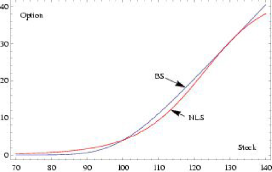
Figure 1: Fitting the Black–Scholes call option with β(w)𝛽𝑤\beta(w)-adaptive PDF of the shock-wave NLS-solution (10).
Refer to caption
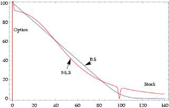
Figure 2: Fitting the Black–Scholes put option with β(w)𝛽𝑤\beta(w)–adaptive PDF of the shock-wave NLS ψ2(s,t)subscript𝜓2𝑠𝑡\psi_{2}(s,t) solution (10). Notice the kink near s=100𝑠100s=100.

Using the standard Kolmogorov probability approach, instead of the market value of an option given by the Black–Scholes equation (1), we could consider the corresponding probability density function (PDF) given by the backward Fokker–Planck equation (see [6, 7]). Alternatively, we can obtain the same PDF (for the market value of a stock option), using the quantum–probability formalism [11, 12], as a solution to a time–dependent linear or nonlinear Schrödinger equation for the evolution of the complex–valued wave ψlimit-from𝜓\psi-function for which the absolute square, |ψ|2,superscript𝜓2|\psi|^{2}, is the PDF. The adaptive nonlinear Schrödinger (NLS) equation was recently used in [10] as an approach to option price modelling, as briefly reviewed in this section. The new model, philosophically founded on adaptive markets hypothesis [13, 14] and Elliott wave market theory [15, 16], as well as my own recent work on quantum congition [17, 18], describes adaptively controlled Brownian market behavior. This nonlinear approach to option price modelling is reviewed in the next section. Its important limiting case with low interest-rate reduces to the linear Schrödinger equation. This linear approach to option price modelling is elaborated in the subsequent section.

2 Nonlinear adaptive wave model for general option pricing

2.1 Adaptive NLS model

The adaptive, wave–form, nonlinear and stochastic option–pricing model with stock price s,𝑠s, volatility σ𝜎\sigma and interest rate r𝑟r is formally defined as a complex-valued, focusing (1+1)–NLS equation, defining the time-dependent option–price wave function ψ=ψ(s,t)𝜓𝜓𝑠𝑡\psi=\psi(s,t), whose absolute square |ψ(s,t)|2superscript𝜓𝑠𝑡2|\psi(s,t)|^{2} represents the probability density function (PDF) for the option price in terms of the stock price and time. In natural quantum units, this NLS equation reads:

itψ=12σssψβ|ψ|2ψ,(i=1),isubscript𝑡𝜓12𝜎subscript𝑠𝑠𝜓𝛽superscript𝜓2𝜓i1\mathrm{i}\partial_{t}\psi=-\frac{1}{2}\sigma\partial_{ss}\psi-\beta|\psi|^{2}\psi,\qquad(\mathrm{i}=\sqrt{-1}),\qquad (5)

where β=β(r,w)𝛽𝛽𝑟𝑤\beta=\beta(r,w) denotes the adaptive market-heat potential (see [19]), so the term V(ψ)=β|ψ|2𝑉𝜓𝛽superscript𝜓2V(\psi)=-\beta|\psi|^{2} represents the ψlimit-from𝜓\psi-dependent potential field. In the simplest nonadaptive scenario β𝛽\beta is equal to the interest rate r𝑟r, while in the adaptive case it depends on the set of adjustable synaptic weights {wji}subscriptsuperscript𝑤𝑖𝑗\{w^{i}_{j}\} as:

β(r,w)=ri=1nw1ierf(w2isw3i).𝛽𝑟𝑤𝑟superscriptsubscript𝑖1𝑛superscriptsubscript𝑤1𝑖erfsuperscriptsubscript𝑤2𝑖𝑠superscriptsubscript𝑤3𝑖\beta(r,w)=r\sum_{i=1}^{n}w_{1}^{i}\,\text{erf}\left(\frac{w_{2}^{i}s}{w_{3}^{i}}\right). (6)

Physically, the NLS equation (5) describes a nonlinear wave (e.g. in Bose-Einstein condensates) defined by the complex-valued wave function ψ(s,t)𝜓𝑠𝑡\psi(s,t) of real space and time parameters. In the present context, the space-like variable s𝑠s denotes the stock (asset) price.

The NLS equation (5) has been exactly solved using the power series expansion method [20, 21] of Jacobi elliptic functions [22]. Consider the ψlimit-from𝜓\psi-function describing a single plane wave, with the wave number k𝑘k and circular frequency ω𝜔\omega:

ψ(s,t)=ϕ(ξ)ei(ksωt),with ξ=sσkt and ϕ(ξ).formulae-sequence𝜓𝑠𝑡italic-ϕ𝜉superscriptei𝑘𝑠𝜔𝑡with 𝜉𝑠𝜎𝑘𝑡 and italic-ϕ𝜉\psi(s,t)=\phi(\xi)\,\mathrm{e}^{\mathrm{i}(ks-\omega t)},\qquad\text{with \ }\xi=s-\sigma kt\text{ \ and \ }\phi(\xi)\in\mathbb{R}. (7)

Its substitution into the NLS equation (5) gives the nonlinear oscillator ODE:

ϕ′′(ξ)+[ω12σk2]ϕ(ξ)+βϕ3(ξ)=0.superscriptitalic-ϕ′′𝜉delimited-[]𝜔12𝜎superscript𝑘2italic-ϕ𝜉𝛽superscriptitalic-ϕ3𝜉0\phi^{\prime\prime}(\xi)+[\omega-\frac{1}{2}\sigma k^{2}]\,\phi(\xi)+\beta\phi^{3}(\xi)=0. (8)

We can seek a solution ϕ(ξ)italic-ϕ𝜉\phi(\xi) for (8) as a linear function [21]

ϕ(ξ)=a0+a1sn(ξ),italic-ϕ𝜉subscript𝑎0subscript𝑎1sn𝜉\phi(\xi)=a_{0}+a_{1}\mathrm{sn}(\xi),

where sn(s)=sn(s,m)sn𝑠sn𝑠𝑚\mathrm{sn}(s)=\mathrm{sn}(s,m) are Jacobi elliptic sine functions with elliptic modulus m[0,1]𝑚01m\in[0,1], such that sn(s,0)=sin(s)sn𝑠0𝑠\mathrm{sn}(s,0)=\sin(s)\ and sn(s,1)=tanh(s)sn𝑠1𝑠\mathrm{sn}(s,1)=\mathrm{\tanh}(s). The solution of (8) was calculated in [10] to be

ϕ(ξ)italic-ϕ𝜉\displaystyle\phi(\xi) =\displaystyle= ±mσβsn(ξ),for m[0,1];andformulae-sequenceplus-or-minus𝑚𝜎𝛽sn𝜉for 𝑚01and\displaystyle\pm m\sqrt{\frac{-\sigma}{\beta}}\,\mathrm{sn}(\xi),\qquad~{}\text{for~{}~{}}m\in[0,1];~{}~{}\text{and}
ϕ(ξ)italic-ϕ𝜉\displaystyle\phi(\xi) =\displaystyle= ±σβtanh(ξ),for m=1.plus-or-minus𝜎𝛽𝜉for 𝑚1\displaystyle\pm\sqrt{\frac{-\sigma}{\beta}}\,\mathrm{\tanh}(\xi),\qquad\text{for~{}~{}}m=1.

This gives the exact periodic solution of (5) as [10]

ψ1(s,t)subscript𝜓1𝑠𝑡\displaystyle\psi_{1}(s,t) =\displaystyle= ±mσβ(w)sn(sσkt)ei[ks12σt(1+m2+k2)],for m[0,1);plus-or-minus𝑚𝜎𝛽𝑤sn𝑠𝜎𝑘𝑡superscripteidelimited-[]𝑘𝑠12𝜎𝑡1superscript𝑚2superscript𝑘2for 𝑚01\displaystyle\pm m\sqrt{\frac{-\sigma}{\beta(w)}}\,\mathrm{sn}(s-\sigma kt)\,\mathrm{e}^{\mathrm{i}[ks-\frac{1}{2}\sigma t(1+m^{2}+k^{2})]},\qquad~{}~{}\text{for~{}~{}}m\in[0,1); (9)
ψ2(s,t)subscript𝜓2𝑠𝑡\displaystyle\psi_{2}(s,t) =\displaystyle= ±σβ(w)tanh(sσkt)ei[ks12σt(2+k2)],for m=1,plus-or-minus𝜎𝛽𝑤𝑠𝜎𝑘𝑡superscripteidelimited-[]𝑘𝑠12𝜎𝑡2superscript𝑘2for 𝑚1\displaystyle\pm\sqrt{\frac{-\sigma}{\beta(w)}}\,\mathrm{\tanh}(s-\sigma kt)\,\mathrm{e}^{\mathrm{i}[ks-\frac{1}{2}\sigma t(2+k^{2})]},\qquad\qquad\text{for~{}~{}}m=1, (10)

where (9) defines the general solution, while (10) defines the envelope shock-wave111A shock wave is a type of fast-propagating nonlinear disturbance that carries energy and can propagate through a medium (or, field). It is characterized by an abrupt, nearly discontinuous change in the characteristics of the medium. The energy of a shock wave dissipates relatively quickly with distance and its entropy increases. On the other hand, a soliton is a self-reinforcing nonlinear solitary wave packet that maintains its shape while it travels at constant speed. It is caused by a cancelation of nonlinear and dispersive effects in the medium (or, field). (or, ‘dark soliton’) solution of the NLS equation (5).

Alternatively, if we seek a solution ϕ(ξ)italic-ϕ𝜉\phi(\xi) as a linear function of Jacobi elliptic cosine functions, such that cn(s,0)=cos(s)cn𝑠0𝑠\mathrm{cn}(s,0)=\cos(s) and cn(s,1)=sech(s)cn𝑠1sech𝑠\mathrm{cn}(s,1)=\mathrm{sech}(s),222A closely related solution of an anharmonic oscillator ODE: ϕ′′(s)+ϕ(s)+ϕ3(s)=0superscriptitalic-ϕ′′𝑠italic-ϕ𝑠superscriptitalic-ϕ3𝑠0\phi^{\prime\prime}(s)+\phi(s)+\phi^{3}(s)=0 is given by ϕ(s)=2m12mcn(1+2m12ms,m).italic-ϕ𝑠2𝑚12𝑚cn12𝑚12𝑚𝑠𝑚\phi(s)=\sqrt{\frac{2m}{1-2m}}\,\text{cn}\left(\sqrt{1+\frac{2m}{1-2m}}~{}s,\,m\right).

ϕ(ξ)=a0+a1cn(ξ),italic-ϕ𝜉subscript𝑎0subscript𝑎1cn𝜉\phi(\xi)=a_{0}+a_{1}\mathrm{cn}(\xi),

then we get [10]

ψ3(s,t)subscript𝜓3𝑠𝑡\displaystyle\psi_{3}(s,t) =\displaystyle= ±mσβ(w)cn(sσkt)ei[ks12σt(12m2+k2)],for m[0,1);plus-or-minus𝑚𝜎𝛽𝑤cn𝑠𝜎𝑘𝑡superscripteidelimited-[]𝑘𝑠12𝜎𝑡12superscript𝑚2superscript𝑘2for 𝑚01\displaystyle\pm m\sqrt{\frac{\sigma}{\beta(w)}}\,\mathrm{cn}(s-\sigma kt)\,\mathrm{e}^{\mathrm{i}[ks-\frac{1}{2}\sigma t(1-2m^{2}+k^{2})]},\qquad\text{for~{}~{}}m\in[0,1); (11)
ψ4(s,t)subscript𝜓4𝑠𝑡\displaystyle\psi_{4}(s,t) =\displaystyle= ±σβ(w)sech(sσkt)ei[ks12σt(k21)],for m=1,plus-or-minus𝜎𝛽𝑤sech𝑠𝜎𝑘𝑡superscripteidelimited-[]𝑘𝑠12𝜎𝑡superscript𝑘21for 𝑚1\displaystyle\pm\sqrt{\frac{\sigma}{\beta(w)}}\,\mathrm{sech}(s-\sigma kt)\,\mathrm{e}^{\mathrm{i}[ks-\frac{1}{2}\sigma t(k^{2}-1)]},\qquad\qquad\text{for~{}~{}}m=1, (12)

where (11) defines the general solution, while (12) defines the envelope solitary-wave (or, ‘bright soliton’) solution of the NLS equation (5).

In all four solution expressions (9), (10), (11) and (12), the adaptive potential β(w)𝛽𝑤\beta(w) is yet to be calculated using either unsupervised Hebbian learning, or supervised Levenberg–Marquardt algorithm (see, e.g. [23, 24]). In this way, the NLS equation (5) becomes the quantum neural network (see [18]). Any kind of numerical analysis can be easily performed using above closed-form solutions ψi(s,t)(i=1,,4)subscript𝜓𝑖𝑠𝑡𝑖14\psi_{i}(s,t)~{}~{}(i=1,...,4) as initial conditions.

The adaptive NLS–PDFs of the shock-wave type (10) has been used in [10] to fit the Black–Scholes call and put options (see Figures 1 and 2). Specifically, the adaptive heat potential (6) was combined with the spatial part of (10)

ϕ(s)=|σβtanh(sktσ)|,2\phi(s)=\left|\sqrt{\frac{\sigma}{\beta}}\tanh(s-kt\sigma)\right|{}^{2}, (13)

while parameter estimates where obtained using 100 iterations of the Levenberg–Marquardt algorithm.
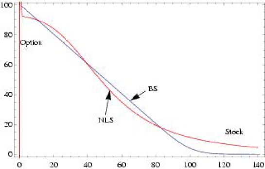
Refer to caption
Figure 3: Smoothing out the kink in the put option fit, by combining the shock-wave solution with the soliton solution, as defined by (14).

As can be seen from Figure (2) there is a kink near s=100𝑠100s=100. This kink, which is a natural characteristic of the spatial shock-wave (13), can be smoothed out (Figure 3) by taking the sum of the spatial parts of the shock-wave solution (10) and the soliton solution (12) as:

ϕ(s)=|σβ[d1tanh(sktσ)+d2sech(sktσ)]|.2\phi(s)=\left|\sqrt{\frac{\sigma}{\beta}}\left[d_{1}\tanh(s-kt\sigma)+d_{2}\,\text{sech}(s-kt\sigma)\right]\right|{}^{2}. (14)

The adaptive NLS–based Greeks (Delta, Rho, Vega, Theta and Gamma) have been defined in [10], as partial derivatives of the shock-wave solution (10).

2.2 Adaptive Manakov system

Next, for the purpose of including a controlled stochastic volatility333Controlled stochastic volatility here represents volatility evolving in a stochastic manner but within the controlled boundaries. into the adaptive–NLS model (5), the full bidirectional quantum neural computation model [18] for option-price forecasting has been formulated in [10] as a self-organized system of two coupled self-focusing NLS equations: one defining the option–price wave function ψ=ψ(s,t)𝜓𝜓𝑠𝑡\psi=\psi(s,t) and the other defining the volatility wave function σ=σ(s,t)𝜎𝜎𝑠𝑡\sigma=\sigma(s,t):

Volatility NLS :itσVolatility NLS :isubscript𝑡𝜎\displaystyle\text{Volatility NLS :}\quad\mathrm{i}\partial_{t}\sigma =\displaystyle= 12ssσβ(r,w)(|σ|2+|ψ|2)σ,12subscript𝑠𝑠𝜎𝛽𝑟𝑤superscript𝜎2superscript𝜓2𝜎\displaystyle-\frac{1}{2}\partial_{ss}\mathcal{\sigma}-\beta(r,w)\left(|\mathcal{\sigma}|^{2}+|\psi|^{2}\right)\mathcal{\sigma}, (15)
Option price NLS :itψOption price NLS :isubscript𝑡𝜓\displaystyle\text{Option price NLS :}\quad\mathrm{i}\partial_{t}\psi =\displaystyle= 12ssψβ(r,w)(|σ|2+|ψ|2)ψ.12subscript𝑠𝑠𝜓𝛽𝑟𝑤superscript𝜎2superscript𝜓2𝜓\displaystyle-\frac{1}{2}\partial_{ss}\psi-\beta(r,w)\left(|\mathcal{\sigma}|^{2}+|\psi|^{2}\right)\psi. (16)

In this coupled model, the σ𝜎\sigma–NLS (15) governs the (s,t)limit-from𝑠𝑡(s,t)-evolution of stochastic volatility, which plays the role of a nonlinear coefficient in (16); the ψ𝜓\psi–NLS (16) defines the (s,t)limit-from𝑠𝑡(s,t)-evolution of option price, which plays the role of a nonlinear coefficient in (15). The purpose of this coupling is to generate a leverage effect, i.e. stock volatility is (negatively) correlated to stock returns444The hypothesis that financial leverage can explain the leverage effect was first discussed by F. Black [26]. (see, e.g. [27]). This bidirectional associative memory effectively performs quantum neural computation [18], by giving a spatio-temporal and quantum generalization of Kosko’s BAM family of neural networks [28, 29]. In addition, the shock-wave and solitary-wave nature of the coupled NLS equations may describe brain-like effects frequently occurring in financial markets: volatility/price propagation, reflection and collision of shock and solitary waves (see [30]).

The coupled NLS-system (15)–(16), without an embedded wlimit-from𝑤w-learning (i.e., for constant β=r𝛽𝑟\beta=r – the interest rate), actually defines the well-known Manakov system,555Manakov system has been used to describe the interaction between wave packets in dispersive conservative media, and also the interaction between orthogonally polarized components in nonlinear optical fibres (see, e.g. [32, 33] and references therein). proven by S. Manakov in 1973 [31] to be completely integrable, by the existence of infinite number of involutive integrals of motion. It admits ‘bright’ and ‘dark’ soliton solutions. The simplest solution of (15)–(16), the so-called Manakov bright 2–soliton, has the form resembling that of the sech-solution (12) (see [34, 35, 36, 37, 38, 39, 40]), and is formally defined by:

ψsol(s,t)=2b𝐜sech(2b(s+4at))e2i(2a2t+as2b2t),subscript𝜓sol𝑠𝑡2𝑏𝐜sech2𝑏𝑠4𝑎𝑡superscripte2i2superscript𝑎2𝑡𝑎𝑠2superscript𝑏2𝑡\mathbf{\psi}_{\mathrm{sol}}(s,t)=2b\,\mathbf{c\,}\mathrm{sech}(2b(s+4at))\,\mathrm{e}^{-2\mathrm{i}(2a^{2}t+as-2b^{2}t)}, (17)

where ψsol(s,t)=(σ(s,t)ψ(s,t))subscript𝜓sol𝑠𝑡𝜎𝑠𝑡𝜓𝑠𝑡\mathbf{\psi}_{\mathrm{sol}}(s,t)=\left(\begin{array}[]{c}\sigma(s,t)\\ \psi(s,t)\end{array}\right), 𝐜=(c1,c2)T𝐜superscriptsubscript𝑐1subscript𝑐2𝑇\mathbf{c}=(c_{1},c_{2})^{T} is a unit vector such that |c1|2+|c2|2=1superscriptsubscript𝑐12superscriptsubscript𝑐221|c_{1}|^{2}+|c_{2}|^{2}=1. Real-valued parameters a𝑎a and b𝑏b are some simple functions of (σ,β,k)𝜎𝛽𝑘(\sigma,\beta,k), which can be determined by the Levenberg–Marquardt algorithm. I have argued in [10] that in some short-time financial situations, the adaptation effect on β𝛽\beta can be neglected, so our option-pricing model (15)–(16) can be reduced to the Manakov 2–soliton model (17), as depicted and explained in Figure 4.
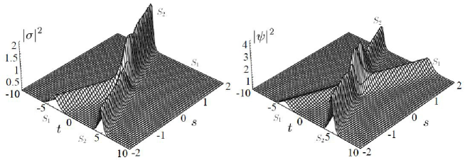
Refer to caption
Figure 4: Hypothetical market scenario including sample PDFs for volatility |σ|2superscript𝜎2|\mathcal{\sigma}|^{2} and |ψ|2superscript𝜓2|\psi|^{2} of the Manakov 2–soliton (17). On the left, we observe the (s,t)limit-from𝑠𝑡(s,t)-evolution of stochastic volatility: we have a collision of two volatility component-solitons, S1(s,t)subscript𝑆1𝑠𝑡S_{1}(s,t) and S2(s,t)subscript𝑆2𝑠𝑡S_{2}(s,t), which join together into the resulting soliton S2(s,t)subscript𝑆2𝑠𝑡S_{2}(s,t), annihilating the S1(s,t)subscript𝑆1𝑠𝑡S_{1}(s,t) component in the process. On the right, we observe the (s,t)limit-from𝑠𝑡(s,t)-evolution of option price: we have a collision of two option component-solitons, S1(s,t)subscript𝑆1𝑠𝑡S_{1}(s,t) and S2(s,t)subscript𝑆2𝑠𝑡S_{2}(s,t), which pass through each other without much change, except at the collision point. Due to symmetry of the Manakov system, volatility and option price can exchange their roles.

3 Quantum wave model for low interest-rate option pricing

In the case of a low interest-rate r1much-less-than𝑟1r\ll 1, we have β(r)1much-less-than𝛽𝑟1\beta(r)\ll 1, so V(ψ)0,𝑉𝜓0V(\psi)\rightarrow 0, and therefore equation (5) can be approximated by a quantum-like option wave packet. It is defined by a continuous superposition of de Broglie’s plane waves, ‘physically’ associated with a free quantum particle of unit mass. This linear wave packet, given by the time-dependent complex-valued wave function ψ=ψ(s,t)𝜓𝜓𝑠𝑡\psi=\psi(s,t), is a solution of the linear Schrödinger equation with zero potential energy, Hamiltonian operator H^^𝐻\hat{H} and volatility σ𝜎\sigma playing the role similar to the Planck constant. This equation can be written as:

iσtψ=H^ψ,whereH^=σ22ss.formulae-sequencei𝜎subscript𝑡𝜓^𝐻𝜓where^𝐻superscript𝜎22subscript𝑠𝑠\mathrm{i}\sigma\partial_{t}\psi=\hat{H}\psi,\qquad\text{where}\qquad\hat{H}=-\frac{\sigma^{2}}{2}\partial_{ss}. (18)

Thus, we consider the ψlimit-from𝜓\psi-function describing a single de Broglie’s plane wave, with the wave number k𝑘k, linear momentum p=σk,𝑝𝜎𝑘p=\sigma k, wavelength λk=2π/k,subscript𝜆𝑘2𝜋𝑘\lambda_{k}=2\pi/k, angular frequency ωk=σk2/2,subscript𝜔𝑘𝜎superscript𝑘22\omega_{k}=\sigma k^{2}/2, and oscillation period Tk=2π/ωk=4π/σk2subscript𝑇𝑘2𝜋subscript𝜔𝑘4𝜋𝜎superscript𝑘2T_{k}=2\pi/\omega_{k}=4\pi/\sigma k^{2}. It is defined by (compare with [41, 42, 12])

ψk(s,t)=Aei(ksωkt)=Aei(ksσk22t)=Acos(ksσk22t)+Aisin(ksσk22t),subscript𝜓𝑘𝑠𝑡𝐴superscriptei𝑘𝑠subscript𝜔𝑘𝑡𝐴superscriptei𝑘𝑠𝜎superscript𝑘22𝑡𝐴𝑘𝑠𝜎superscript𝑘22𝑡𝐴i𝑘𝑠𝜎superscript𝑘22𝑡\psi_{k}(s,t)=A\mathrm{e}^{\mathrm{i}(ks-\omega_{k}t)}=A\mathrm{e}^{\mathrm{i}(ks-{\frac{\sigma k^{2}}{2}}t)}=A\cos(ks-{\frac{\sigma k^{2}}{2}}t)+A\mathrm{i}\sin(ks-{\frac{\sigma k^{2}}{2}}t), (19)

where A𝐴A is the amplitude of the wave, the angle (ksωkt)=(ksσk22t)𝑘𝑠subscript𝜔𝑘𝑡𝑘𝑠𝜎superscript𝑘22𝑡(ks-\omega_{k}t)=(ks-{\frac{\sigma k^{2}}{2}}t) represents the phase of the wave ψksubscript𝜓𝑘\psi_{k} with the phase velocity: vk=ωk/k=σk/2.subscript𝑣𝑘subscript𝜔𝑘𝑘𝜎𝑘2v_{k}=\omega_{k}/k=\sigma k/2.

The space-time wave function ψ(s,t)𝜓𝑠𝑡\psi(s,t) that satisfies the linear Schrödinger equation (18) can be decomposed (using Fourier’s separation of variables) into the spatial part ϕ(s)italic-ϕ𝑠\phi(s)\, and the temporal part eiωtsuperscriptei𝜔𝑡\mathrm{e}^{-\mathrm{i}\omega t}\ as:

ψ(s,t)=ϕ(s)eiωt=ϕ(s)eiσEt.𝜓𝑠𝑡italic-ϕ𝑠superscriptei𝜔𝑡italic-ϕ𝑠superscriptei𝜎𝐸𝑡\psi(s,t)=\phi(s)\,\mathrm{e}^{-\mathrm{i}\omega t}=\phi(s)\,\mathrm{e}^{-\frac{\mathrm{i}}{\sigma}Et}.

The spatial part, representing stationary (or, amplitude) wave function, ϕ(s)=Aeiks,italic-ϕ𝑠𝐴superscriptei𝑘𝑠\phi(s)=A\mathrm{e}^{\mathrm{i}ks}, satisfies the linear harmonic oscillator, which can be formulated in several equivalent forms:

ϕ′′+k2ϕ=0,ϕ′′+(pσ)2ϕ=0,ϕ′′+(ωkvk)2ϕ=0,ϕ′′+2Ekσ2ϕ=0.formulae-sequencesuperscriptitalic-ϕ′′superscript𝑘2italic-ϕ0formulae-sequencesuperscriptitalic-ϕ′′superscript𝑝𝜎2italic-ϕ0formulae-sequencesuperscriptitalic-ϕ′′superscriptsubscript𝜔𝑘subscript𝑣𝑘2italic-ϕ0superscriptitalic-ϕ′′2subscript𝐸𝑘superscript𝜎2italic-ϕ0\phi^{\prime\prime}+k^{2}\phi=0,\qquad\phi^{\prime\prime}+\left(\frac{p}{\sigma}\right)^{2}\phi=0,\qquad\phi^{\prime\prime}+\left(\frac{\omega_{k}}{v_{k}}\right)^{2}\phi=0,\qquad\phi^{\prime\prime}+\frac{2E_{k}}{\sigma^{2}}\phi=0. (20)

Planck’s energy quantum of the option wave ψksubscript𝜓𝑘\psi_{k} is given by: Ek=σωk=12(σk)2.subscript𝐸𝑘𝜎subscript𝜔𝑘12superscript𝜎𝑘2E_{k}=\sigma\omega_{k}=\frac{1}{2}(\sigma k)^{2}.

From the plane-wave expressions (19) we have: ψk(s,t)=Aeiσ(psEkt)subscript𝜓𝑘𝑠𝑡limit-from𝐴superscriptei𝜎𝑝𝑠subscript𝐸𝑘𝑡\psi_{k}(s,t)=A\mathrm{e}^{\frac{\mathrm{i}}{\sigma}(ps-E_{k}t)}- for the wave going to the ‘right’ and ψk(s,t)=Aeiσ(ps+Ekt)subscript𝜓𝑘𝑠𝑡limit-from𝐴superscriptei𝜎𝑝𝑠subscript𝐸𝑘𝑡\psi_{k}(s,t)=A\mathrm{e}^{-\frac{\mathrm{i}}{\sigma}(ps+E_{k}t)}- for the wave going to the ‘left’.

The general solution to (18) is formulated as a linear combination of de Broglie’s option waves (19), comprising the option wave-packet:

ψ(s,t)=i=0nciψki(s,t),(withn).𝜓𝑠𝑡superscriptsubscript𝑖0𝑛subscript𝑐𝑖subscript𝜓subscript𝑘𝑖𝑠𝑡with𝑛\psi(s,t)=\sum_{i=0}^{n}c_{i}\psi_{k_{i}}(s,t),\qquad(\text{with}\ n\in\mathbb{N}). (21)

Its absolute square, |ψ(s,t)|2,superscript𝜓𝑠𝑡2|\psi(s,t)|^{2}, represents the probability density function at a time t.𝑡t.

The group velocity of an option wave-packet is given by: vg=dωk/dk.subscript𝑣𝑔𝑑subscript𝜔𝑘𝑑𝑘\ v_{g}=d\omega_{k}/dk. It is related to the phase velocity vksubscript𝑣𝑘v_{k} of a plane wave as: vg=vkλkdvk/dλk.subscript𝑣𝑔subscript𝑣𝑘subscript𝜆𝑘𝑑subscript𝑣𝑘𝑑subscript𝜆𝑘v_{g}=v_{k}-\lambda_{k}dv_{k}/d\lambda_{k}. Closely related is the center of the option wave-packet (the point of maximum amplitude), given by: s=tdωk/dk.𝑠𝑡𝑑subscript𝜔𝑘𝑑𝑘s=td\omega_{k}/dk.

The following quantum-motivated assertions can be stated:

  1. 1.

    Volatility σ𝜎\sigma has dimension of financial action, or energy ×\times time.

  2. 2.

    The total energy E𝐸E of an option wave-packet is (in the case of similar plane waves) given by Planck’s superposition of the energies Eksubscript𝐸𝑘E_{k} of n𝑛n individual waves: E=nσωk=n2(σk)2,𝐸𝑛𝜎subscript𝜔𝑘𝑛2superscript𝜎𝑘2E=n\sigma\omega_{k}=\frac{n}{2}(\sigma k)^{2}, where L=nσ𝐿𝑛𝜎L=n\sigma denotes the angular momentum of the option wave-packet, representing the shift between its growth and decay, and vice versa.

  3. 3.

    The average energy Edelimited-⟨⟩𝐸\left\langle E\right\rangle of an option wave-packet is given by Boltzmann’s partition function:

    E=n=0nEkenEkbTn=0enEkbT=EkeEkbT1,delimited-⟨⟩𝐸superscriptsubscript𝑛0𝑛subscript𝐸𝑘superscripte𝑛subscript𝐸𝑘𝑏𝑇superscriptsubscript𝑛0superscripte𝑛subscript𝐸𝑘𝑏𝑇subscript𝐸𝑘superscriptesubscript𝐸𝑘𝑏𝑇1\left\langle E\right\rangle=\frac{\sum_{n=0}^{\infty}nE_{k}\mathrm{e}^{-\frac{nE_{k}}{bT}}}{\sum_{n=0}^{\infty}\mathrm{e}^{-\frac{nE_{k}}{bT}}}=\frac{E_{k}}{\mathrm{e}^{\frac{E_{k}}{bT}}-1},

    where b𝑏b is the Boltzmann-like kinetic constant and T𝑇T is the market temperature.

  4. 4.

    The energy form of the Schrödinger equation (18) reads: Eψ=iσtψ𝐸𝜓i𝜎subscript𝑡𝜓E\psi=\mathrm{i}\sigma\partial_{t}\psi.

  5. 5.

    The eigenvalue equation for the Hamiltonian operator H^^𝐻\hat{H} is the stationary Schrödinger equation:

    H^ϕ(s)=Eϕ(s),orEϕ(s)=σ22ssϕ(s),formulae-sequence^𝐻italic-ϕ𝑠𝐸italic-ϕ𝑠or𝐸italic-ϕ𝑠superscript𝜎22subscript𝑠𝑠italic-ϕ𝑠\hat{H}\phi(s)=E\phi(s),\qquad\text{or}\qquad E\phi(s)=-\frac{\sigma^{2}}{2}\partial_{ss}\phi(s),

    which is just another form of the harmonic oscillator (20). It has oscillatory solutions of the form:

    ϕE(s)=c1eiσ2Eks+c2eiσ2Eks,subscriptitalic-ϕ𝐸𝑠subscript𝑐1superscriptei𝜎2subscript𝐸𝑘𝑠subscript𝑐2superscriptei𝜎2subscript𝐸𝑘𝑠\phi_{E}(s)=c_{1}\mathrm{e}^{\frac{\mathrm{i}}{\sigma}\sqrt{2E_{k}}\,s}+c_{2}\mathrm{e}^{-\frac{\mathrm{i}}{\sigma}\sqrt{2E_{k}}\,s}\,,

    called energy eigen-states with energies Eksubscript𝐸𝑘E_{k} and denoted by: H^ϕE(s)=EkϕE(s).^𝐻subscriptitalic-ϕ𝐸𝑠subscript𝐸𝑘subscriptitalic-ϕ𝐸𝑠\hat{H}\phi_{E}(s)=E_{k}\phi_{E}(s).

Refer to caption
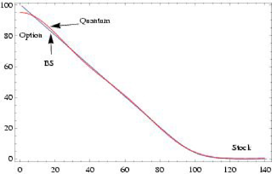
Figure 5: Fitting the Black–Scholes put option with the quantum PDF given by the absolute square of (21) with n=7𝑛7n=7.
Refer to caption
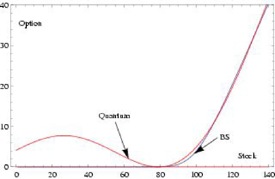
Figure 6: Fitting the Black–Scholes call option with the quantum PDF given by the absolute square of (21) with n=3𝑛3n=3. Note that fit is good in the realistic stock region: s[75,140]𝑠75140s\in[75,140].

The Black–Scholes put and call options have been fitted with the quantum PDFs (see Figures 5 and 6) given by the absolute square of (21) with n=7𝑛7n=7 and n=3𝑛3n=3, respectively. Using supervised Levenberg–Marquardt algorithm and Mathematica 7, the following coefficients were obtained for the Black–Scholes put option:

σ=0.0031891,t=0.0031891,k1=2.62771,k2=2.62777,k3=2.65402,formulae-sequencesuperscript𝜎0.0031891formulae-sequencesuperscript𝑡0.0031891formulae-sequencesubscript𝑘12.62771formulae-sequencesubscript𝑘22.62777subscript𝑘32.65402\sigma^{*}=-0.0031891,~{}t^{*}=-0.0031891,~{}k_{1}=2.62771,~{}k_{2}=2.62777,~{}k_{3}=2.65402,

k4=2.61118,k5=2.64104,k6=2.54737,k7=2.62778,c1=1.26632,c2=1.26517,formulae-sequencesubscript𝑘42.61118formulae-sequencesubscript𝑘52.64104formulae-sequencesubscript𝑘62.54737formulae-sequencesubscript𝑘72.62778formulae-sequencesubscript𝑐11.26632subscript𝑐21.26517k_{4}=2.61118,~{}k_{5}=2.64104,~{}k_{6}=2.54737,~{}k_{7}=2.62778,~{}c_{1}=1.26632,~{}c_{2}=1.26517,

c3=2.74379,c4=1.35495,c5=1.59586,c6=0.263832,c7=1.26779,formulae-sequencesubscript𝑐32.74379formulae-sequencesubscript𝑐41.35495formulae-sequencesubscript𝑐51.59586formulae-sequencesubscript𝑐60.263832subscript𝑐71.26779c_{3}=2.74379,~{}c_{4}=1.35495,~{}c_{5}=1.59586,~{}c_{6}=0.263832,~{}c_{7}=1.26779,

with  σBS=94.0705σ,tBS=31.3568t.formulae-sequencesubscript𝜎𝐵𝑆94.0705superscript𝜎subscript𝑡𝐵𝑆31.3568superscript𝑡\sigma_{BS}=-94.0705\sigma^{*},~{}t_{BS}=-31.3568t^{*}.

Using the same algorithm, the following coefficients were obtained for the Black–Scholes call option:

σ=11.9245,t=11.9245,k1=0.851858,k2=0.832409,formulae-sequencesuperscript𝜎11.9245formulae-sequencesuperscript𝑡11.9245formulae-sequencesubscript𝑘10.851858subscript𝑘20.832409\sigma^{*}=-11.9245,~{}t^{*}=-11.9245,~{}k_{1}=0.851858,~{}k_{2}=0.832409,

k3=0.872061,c1=2.9004,c2=2.72592,c3=2.93291,formulae-sequencesubscript𝑘30.872061formulae-sequencesubscript𝑐12.9004formulae-sequencesubscript𝑐22.72592subscript𝑐32.93291k_{3}=0.872061,~{}c_{1}=2.9004,~{}c_{2}=2.72592,~{}c_{3}=2.93291,

with σBS0.0251583σ,t=0.00838609t.subscript𝜎𝐵𝑆0.0251583superscript𝜎𝑡0.00838609superscript𝑡\sigma_{BS}-0.0251583\sigma^{*},~{}t=-0.00838609t^{*}.

Now, given some initial option wave function, ψ(s,0)=ψ0(s),𝜓𝑠0subscript𝜓0𝑠\psi(s,0)=\psi_{0}(s), a solution to the initial-value problem for the linear Schrödinger equation (18) is, in terms of the pair of Fourier transforms (,1),superscript1(\mathcal{F},\mathcal{F}^{-1}), given by (see [42])

ψ(s,t)=1[eiωt(ψ0)]=1[eiσk22t(ψ0)].𝜓𝑠𝑡superscript1delimited-[]superscriptei𝜔𝑡subscript𝜓0superscript1delimited-[]superscriptei𝜎superscript𝑘22𝑡subscript𝜓0\psi(s,t)=\mathcal{F}^{-1}\left[\mathrm{e}^{-\mathrm{i}\omega t}\mathcal{F}(\psi_{0})\right]=\mathcal{F}^{-1}\left[\mathrm{e}^{-\mathrm{i}{\frac{\sigma k^{2}}{2}}t}\mathcal{F}(\psi_{0})\right]. (22)

For example (see [42]), suppose we have an initial option wave-function at time t=0𝑡0t=0 given by the complex-valued Gaussian function:

ψ(s,0)=eas2/2eiσks,𝜓𝑠0superscripte𝑎superscript𝑠22superscriptei𝜎𝑘𝑠\psi(s,0)=\mathrm{e}^{-as^{2}/2}\mathrm{e}^{\mathrm{i}\sigma ks},

where a𝑎a is the width of the Gaussian, while p𝑝p is the average momentum of the wave. Its Fourier transform, ψ^0(k)=[ψ(s,0)],subscript^𝜓0𝑘delimited-[]𝜓𝑠0\hat{\psi}_{0}(k)=\mathcal{F}[\psi(s,0)], is given by

ψ^0(k)=e(kp)22aa.subscript^𝜓0𝑘superscriptesuperscript𝑘𝑝22𝑎𝑎\hat{\psi}_{0}(k)=\frac{\mathrm{e}^{-\frac{(k-p)^{2}}{2a}}}{\sqrt{a}}.

The solution at time t𝑡t of the initial value problem is given by

ψ(s,t)=12πa+ei(ksσk22t)ea(kp)22a𝑑k,𝜓𝑠𝑡12𝜋𝑎superscriptsubscriptsuperscriptei𝑘𝑠𝜎superscript𝑘22𝑡superscripte𝑎superscript𝑘𝑝22𝑎differential-d𝑘\psi(s,t)=\frac{1}{\sqrt{2\pi a}}\int_{-\infty}^{+\infty}\mathrm{e}^{\mathrm{i}(ks-{\frac{\sigma k^{2}}{2}}t)}\,\mathrm{e}^{-\frac{a(k-p)^{2}}{2a}}\,dk,

which, after some algebra becomes

ψ(s,t)=exp(as22isp+ip2t2(1+iat))1+iat,(with p=σk).𝜓𝑠𝑡𝑎superscript𝑠22i𝑠𝑝isuperscript𝑝2𝑡21i𝑎𝑡1i𝑎𝑡with 𝑝𝜎𝑘\psi(s,t)=\frac{\mathrm{\exp}(-\frac{as^{2}-2\mathrm{i}sp+\mathrm{i}p^{2}t}{2(1+\mathrm{i}at)})}{\sqrt{1+\mathrm{i}at}},\qquad(\text{with \ }p=\sigma k).

As a simpler example,666An example of a more general Gaussian wave-packet solution of (18) is given by: ψ(s,t)=a/π1+iatexp(12a(ss0)2i2p02t+ip0(ss0)1+iat),𝜓𝑠𝑡𝑎𝜋1i𝑎𝑡12𝑎superscript𝑠subscript𝑠02i2superscriptsubscript𝑝02𝑡isubscript𝑝0𝑠subscript𝑠01i𝑎𝑡\psi(s,t)=\sqrt{\frac{\sqrt{a/\pi}}{1+\mathrm{i}at}}\,\exp\left(\frac{-\frac{1}{2}a(s-{s_{0}})^{2}-\frac{\mathrm{i}}{2}p_{0}^{2}t+\mathrm{i}p_{0}(s-{s_{0}})}{1+\mathrm{i}at}\right), where s0,p0subscript𝑠0subscript𝑝0s_{0},p_{0} are initial stock-price and average momentum, while a𝑎a is the width of the Gaussian. At time t=0𝑡0t=0 the ‘particle’ is at rest around s=0𝑠0s=0, its average momentum p0=0subscript𝑝00p_{0}=0. The wave function spreads with time while its maximum decreases and stays put at the origin. At time t𝑡-t the wave packet is the complex-conjugate of the wave-packet at time t𝑡t. if we have an initial option wave-function given by the real-valued Gaussian function,

ψ(s,0)=es2/2π4,𝜓𝑠0superscriptesuperscript𝑠224𝜋\psi(s,0)=\frac{\mathrm{e}^{-s^{2}/2}}{\sqrt[4]{\pi}},

the solution of (18) is given by the complex-valued ψlimit-from𝜓\psi-function,

ψ(s,t)=exp(s22(1+it))π41+it.𝜓𝑠𝑡superscript𝑠221i𝑡4𝜋1i𝑡\psi(s,t)=\frac{\mathrm{\exp}(-\frac{s^{2}}{2(1+\mathrm{i}t)})}{\sqrt[4]{\pi}\sqrt{1+\mathrm{i}t}}.

From (22) it follows that a stationary option wave-packet is given by:

ϕ(s)=12π+eiσksψ^(k)𝑑k,whereψ^(k)=[ϕ(s)].formulae-sequenceitalic-ϕ𝑠12𝜋superscriptsubscriptsuperscriptei𝜎𝑘𝑠^𝜓𝑘differential-d𝑘where^𝜓𝑘delimited-[]italic-ϕ𝑠\phi(s)=\frac{1}{\sqrt{2\pi}}\int_{-\infty}^{+\infty}\mathrm{e}^{\frac{\mathrm{i}}{\sigma}ks}\,\hat{\psi}(k)\,dk,\qquad\text{where}\qquad\hat{\psi}(k)=\mathcal{F}[\phi(s)].

As |ϕ(s)|2superscriptitalic-ϕ𝑠2|\phi(s)|^{2} is the stationary stock PDF, we can calculate the expectation values of the stock and the wave number of the whole option wave-packet, consisting of n𝑛n measured plane waves, as:

s=+s|ϕ(s)|2𝑑sandk=+k|ψ^(k)|2𝑑k.formulae-sequencedelimited-⟨⟩𝑠superscriptsubscript𝑠superscriptitalic-ϕ𝑠2differential-d𝑠anddelimited-⟨⟩𝑘superscriptsubscript𝑘superscript^𝜓𝑘2differential-d𝑘\left\langle s\right\rangle=\int_{-\infty}^{+\infty}s|\phi(s)|^{2}ds\qquad\text{and}\qquad\left\langle k\right\rangle=\int_{-\infty}^{+\infty}k|\hat{\psi}(k)|^{2}dk. (23)

The recordings of n𝑛n individual option plane waves (19) will be scattered around the mean values (23). The width of the distribution of the recorded slimit-from𝑠s- and klimit-from𝑘k-values are uncertainties ΔsΔ𝑠\Delta s and Δk,Δ𝑘\Delta k, respectively. They satisfy the Heisenberg-type uncertainty relation:

ΔsΔkn2,Δ𝑠Δ𝑘𝑛2\Delta s\,\Delta k\geq\frac{n}{2},

which imply the similar relation for the total option energy and time:

ΔEΔtn2.Δ𝐸Δ𝑡𝑛2\Delta E\,\Delta t\geq\frac{n}{2}.

Finally, Greeks for both put and call options are defined as the following partial derivatives of the option ψlimit-from𝜓\psi-function PDF:

Delta=s|ψ(s,t)|2=2ij=1ncjkjekj(is12iσkjt)Abs[j=1ncjekj(is12iσkjt)]Abs[j=1ncjekj(is12iσkjt)]Deltasubscript𝑠superscript𝜓𝑠𝑡22isuperscriptsubscript𝑗1𝑛subscript𝑐𝑗subscript𝑘𝑗superscriptesubscript𝑘𝑗i𝑠12i𝜎subscript𝑘𝑗𝑡Absdelimited-[]superscriptsubscript𝑗1𝑛subscript𝑐𝑗superscriptesubscript𝑘𝑗i𝑠12i𝜎subscript𝑘𝑗𝑡superscriptAbsdelimited-[]superscriptsubscript𝑗1𝑛subscript𝑐𝑗superscriptesubscript𝑘𝑗i𝑠12i𝜎subscript𝑘𝑗𝑡{\text{Delta}}=\partial_{s}|\psi(s,t)|^{2}=\newline {2\mathrm{i}\sum_{j=1}^{n}c_{j}k_{j}\,\mathrm{e}^{k_{j}\left(\mathrm{i}s-\text{${\frac{1}{2}}$}\mathrm{i}\sigma k_{j}t\right)}\text{Abs}\left[\sum_{j=1}^{n}c_{j}\,\mathrm{e}^{k_{j}\left(\mathrm{i}s-\text{${\frac{1}{2}}$}\mathrm{i}\sigma k_{j}t\right)}\right]\text{Abs}^{\prime}\left[\sum_{j=1}^{n}c_{j}\,\mathrm{e}^{k_{j}\left(\mathrm{i}s-\text{${\frac{1}{2}}$}\mathrm{i}\sigma k_{j}t\right)}\right]}

Vega=σ|ψ(s,t)|2=itj=1ncjkjekj(is12iσkjt)2Abs[j=1ncjekj(is12iσkjt)]Abs[j=1ncjekj(is12iσkjt)]Vegasubscript𝜎superscript𝜓𝑠𝑡2itsuperscriptsubscript𝑗1𝑛subscript𝑐𝑗subscript𝑘𝑗superscriptsuperscriptesubscript𝑘𝑗i𝑠12i𝜎subscript𝑘𝑗𝑡2Absdelimited-[]superscriptsubscript𝑗1𝑛subscript𝑐𝑗superscriptesubscript𝑘𝑗i𝑠12i𝜎subscript𝑘𝑗𝑡superscriptAbsdelimited-[]superscriptsubscript𝑗1𝑛subscript𝑐𝑗superscriptesubscript𝑘𝑗i𝑠12i𝜎subscript𝑘𝑗𝑡{\text{Vega}}=\partial_{{\text{$\sigma$}}}|\psi(s,t)|^{2}=\newline {-\text{it}\sum_{j=1}^{n}c_{j}k_{j}{}^{2}\,\mathrm{e}^{k_{j}\left(\mathrm{i}s-\text{${\frac{1}{2}}$}\mathrm{i}\sigma k_{j}t\right)}\text{Abs}\left[\sum_{j=1}^{n}c_{j}\,\mathrm{e}^{k_{j}\left(\mathrm{i}s-\text{${\frac{1}{2}}$}\mathrm{i}\sigma k_{j}t\right)}\right]\text{Abs}^{\prime}\left[\sum_{j=1}^{n}c_{j}\,\mathrm{e}^{k_{j}\left(\mathrm{i}s-\text{${\frac{1}{2}}$}\mathrm{i}\sigma k_{j}t\right)}\right]}

Theta=t|ψ(s,t)|2=iσj=1ncjkjekj(is12iσkjt)2Abs[j=1ncjekj(is12iσkjt)]Abs[j=1ncjekj(is12iσkjt)]Thetasubscript𝑡superscript𝜓𝑠𝑡2iσsuperscriptsubscript𝑗1𝑛subscript𝑐𝑗subscript𝑘𝑗superscriptsuperscriptesubscript𝑘𝑗i𝑠12i𝜎subscript𝑘𝑗𝑡2Absdelimited-[]superscriptsubscript𝑗1𝑛subscript𝑐𝑗superscriptesubscript𝑘𝑗i𝑠12i𝜎subscript𝑘𝑗𝑡superscriptAbsdelimited-[]superscriptsubscript𝑗1𝑛subscript𝑐𝑗superscriptesubscript𝑘𝑗i𝑠12i𝜎subscript𝑘𝑗𝑡{\text{Theta}}=\partial_{{\text{$t$}}}|\psi(s,t)|^{2}=\newline {-\text{{i}$\sigma$}\sum_{j=1}^{n}c_{j}k_{j}{}^{2}\,\mathrm{e}^{k_{j}\left(\mathrm{i}s-\text{${\frac{1}{2}}$}\mathrm{i}\sigma k_{j}t\right)}\text{Abs}\left[\sum_{j=1}^{n}c_{j}\,\mathrm{e}^{k_{j}\left(\mathrm{i}s-\text{${\frac{1}{2}}$}\mathrm{i}\sigma k_{j}t\right)}\right]\text{Abs}^{\prime}\left[\sum_{j=1}^{n}c_{j}\,\mathrm{e}^{k_{j}\left(\mathrm{i}s-\text{${\frac{1}{2}}$}\mathrm{i}\sigma k_{j}t\right)}\right]}

Gamma=ss|ψ(s,t)|2=2j=1ncjkjekj(is12iσkjt)2Abs[j=1ncjekj(is12iσkjt)]Abs[j=1ncjekj(is12iσkjt)](j=1ncjkjekj(is12iσkjt))Abs2[j=1ncjekj(is12iσkjt)]2(j=1ncjkjekj(is12iσkjt))Abs2[j=1ncjekj(is12iσkjt)]Abs′′[j=1ncjekj(is12iσkjt)],{\text{Gamma}}=\partial_{ss}|\psi(s,t)|^{2}=\newline {-2\sum_{j=1}^{n}c_{j}k_{j}{}^{2}\,\mathrm{e}^{k_{j}\left(\mathrm{i}s-\text{${\frac{1}{2}}$}\mathrm{i}\sigma k_{j}t\right)}\text{Abs}\left[\sum_{j=1}^{n}c_{j}\,\mathrm{e}^{k_{j}\left(\mathrm{i}s-\text{${\frac{1}{2}}$}\mathrm{i}\sigma k_{j}t\right)}\right]\text{Abs}^{\prime}\left[\sum_{j=1}^{n}c_{j}\,\mathrm{e}^{k_{j}\left(\mathrm{i}s-\text{${\frac{1}{2}}$}\mathrm{i}\sigma k_{j}t\right)}\right]-}\newline {\left(\sum_{j=1}^{n}c_{j}k_{j}\,\mathrm{e}^{k_{j}\left(\mathrm{i}s-\text{${\frac{1}{2}}$}\mathrm{i}\sigma k_{j}t\right)}\right){}^{2}\text{Abs}^{\prime}\left[\sum_{j=1}^{n}c_{j}\,\mathrm{e}^{k_{j}\left(\mathrm{i}s-\text{${\frac{1}{2}}$}\mathrm{i}\sigma k_{j}t\right)}\right]{}^{2}-}\newline {\left(\sum_{j=1}^{n}c_{j}k_{j}\,\mathrm{e}^{k_{j}\left(\mathrm{i}s-\text{${\frac{1}{2}}$}\mathrm{i}\sigma k_{j}t\right)}\right){}^{2}\text{Abs}\left[\sum_{j=1}^{n}c_{j}\,\mathrm{e}^{k_{j}\left(\mathrm{i}s-\text{${\frac{1}{2}}$}\mathrm{i}\sigma k_{j}t\right)}\right]\text{Abs}^{\prime\prime}\left[\sum_{j=1}^{n}c_{j}\,\mathrm{e}^{k_{j}\left(\mathrm{i}s-\text{${\frac{1}{2}}$}\mathrm{i}\sigma k_{j}t\right)}\right]},

where Abs denotes the absolute value, while AbssuperscriptAbs\text{Abs}^{\prime} and Abs′′superscriptAbs′′\text{Abs}^{\prime\prime} denote its first and second derivatives.

4 Conclusion

I have proposed an adaptive–wave alternative to the standard Black-Scholes option pricing model. The new model, philosophically founded on adaptive markets hypothesis [13, 14] and Elliott wave market theory [15, 16], describes adaptively controlled Brownian market behavior. Two approaches have been proposed: (i) a nonlinear one based on the adaptive NLS (solved by means of Jacobi elliptic functions) and the adaptive Manakov system (of two coupled NLS equations); (ii) a linear quantum-mechanical one based on the free-particle Schrödinger equation and de Broglie’s plane waves. For the purpose of fitting the Black-Scholes data, the Levenberg-Marquardt algorithm was used.

The presented adaptive and quantum wave models are spatio-temporal dynamical systems of much higher complexity [25] then the Black-Scholes model. This makes the new wave models harder to analyze, but at the same time, their immense variety is potentially much closer to the real financial market complexity, especially at the time of financial crisis.

References

  • [1] F. Black, M. Scholes, The Pricing of Options and Corporate Liabilities, J. Pol. Econ. 81, 637-659, (1973)
  • [2] R.C. Merton, Bell J. Econ. and Management Sci. 4, 141-183, (1973)
  • [3] M.F.M. Osborne, Operations Research 7, 145-173, (1959)
  • [4] K. Itô, Mem. Am. Math. Soc. 4, 1-51, (1951)
  • [5] J. Perello, J. M. Porra, M. Montero, J. Masoliver, Physica A 278, 1-2, 260-274, (2000)
  • [6] C.W. Gardiner, Handbook of Stochastic Methods, Springer, Berlin, (1983)
  • [7] J. Voit, The Statistical Mechanics of Financial Markets. Springer, (2005)
  • [8] R.L. Stratonovich, SIAM J. Control 4, 362-371, (1966)
  • [9] M. Kelly, Black-Scholes Option Model & European Option Greeks. The Wolfram Demonstrations Project, http://demonstrations.wolfram.com/EuropeanOptionGreeks, (2009)
  • [10] V. Ivancevic, Cogn. Comput. (in press) arXiv.q-fin.PR:0911.1834
  • [11] V. Ivancevic, T. Ivancevic, Complex Dynamics: Advanced System Dynamics in Complex Variables. Springer, Dordrecht, (2007)
  • [12] V. Ivancevic, T. Ivancevic, Quantum Leap: From Dirac and Feynman, Across the Universe, to Human Body and Mind. World Scientific, Singapore, (2008)
  • [13] A.W. Lo, J. Portf. Manag. 30, 15-29, (2004)
  • [14] A.W. Lo, J. Inves. Consult. 7, 21-44, (2005)
  • [15] A.J. Frost, R.R. Prechter, Jr., Elliott Wave Principle: Key to Market Behavior. Wiley, New York, (1978); (10th Edition) Elliott Wave International, (2009)
  • [16] P. Steven, Applying Elliott Wave Theory Profitably. Wiley, New York, (2003)
  • [17] V. Ivancevic, E. Aidman, Physica A 382, 616–630, (2007)
  • [18] V. Ivancevic, T. Ivancevic, Quantum Neural Computation, Springer, (2009)
  • [19] H. Kleinert, H. Kleinert, Path Integrals in Quantum Mechanics, Statistics, Polymer Physics, and Financial Markets (3rd ed), World Scientific, Singapore, (2002)
  • [20] S. Liu, Z. Fu, S. Liu, Q. Zhao, Phys. Let. A 289, 69–74, (2001)
  • [21] G-T. Liu, T-Y. Fan, Phys. Let. A 345, 161–166, (2005)
  • [22] M. Abramowitz, I.A. Stegun, (Eds): Jacobian Elliptic Functions and Theta Functions. Chapter 16 in Handbook of Mathematical Functions with Formulas, Graphs, and Mathematical Tables (9th ed). Dover, New York, 567-581, (1972)
  • [23] V. Ivancevic, T. Ivancevic, Neuro-Fuzzy Associative Machinery for Comprehensive Brain and Cognition Modelling. Springer, Berlin, (2007)
  • [24] V. Ivancevic, T. Ivancevic, Computational Mind: A Complex Dynamics Perspective. Springer, Berlin, (2007)
  • [25] V. Ivancevic, T. Ivancevic, Complex Nonlinearity: Chaos, Phase Transitions, Topology Change and Path Integrals, Springer, (2008)
  • [26] F. Black, 1976 Meet. Ame. Stat. Assoc. Bus. Econ. Stat. 177—181, (1976)
  • [27] H.E. Roman, M. Porto, C. Dose, EPL 84, 28001, (5pp), (2008)
  • [28] B. Kosko, IEEE Trans. Sys. Man Cyb. 18, 49–60, (1988)
  • [29] B. Kosko, Neural Networks, Fuzzy Systems, A Dynamical Systems Approach to Machine Intelligence. Prentice–Hall, New York, (1992)
  • [30] S.-H. Hanm, I.G. Koh, Phys. Rev. E 60, 7608–7611, (1999)
  • [31] S.V. Manakov, (in Russian) Zh. Eksp. Teor. Fiz. 65 505?516, (1973); (transleted into English) Sov. Phys. JETP 38, 248–253, (1974)
  • [32] M. Haelterman, A.P. Sheppard, Phys. Rev. E 49, 3376?3381, (1994)
  • [33] J. Yang, Physica D 108, 92?112, (1997)
  • [34] D.J. Benney, A.C. Newell, J. Math. Phys. 46, 133-139, (1967)
  • [35] V.E. Zakharov, S.V. Manakov, S.P. Novikov, L.P. Pitaevskii, Soliton theory: inverse scattering method. Nauka, Moscow, (1980)
  • [36] A. Hasegawa, Y. Kodama, Solitons in Optical Communications. Clarendon, Oxford, (1995)
  • [37] R. Radhakrishnan, M. Lakshmanan, J. Hietarinta, Phys. Rev. E. 56, 2213, (1997)
  • [38] G. Agrawal, Nonlinear fiber optics (3rd ed.). Academic Press, San Diego, (2001).
  • [39] J. Yang, Phys. Rev. E 64, 026607, (2001)
  • [40] J. Elgin, V. Enolski, A. Its, Physica D 225 (22), 127-152, (2007)
  • [41] D.J. Griffiths, Introduction to Quantum Mechanics (2nd ed.), Pearson Educ. Int., (2005)
  • [42] B. Thaller, Visual Quantum Mechanics, Springer, New York, (2000)