AO Vel: The role of multiplicity in the development of chemical peculiarities in late B-type stars

Abstract

We present high-resolution, high signal-to-noise UVES spectra of AO Vel, a quadruple system containing an eclipsing BpSi star. From these observations we reconstruct the spectra of the individual components and perform an abundance analysis of all four stellar members. We found that all components are chemically peculiar with different abundances patters. In particular, the two less massive stars show typical characteristics of HgMn stars. The two most massive stars in the system show variable line profiles indicating the presence of chemical spots. Given the youth of the system and the notable chemical peculiarities of their components, this system could give important insights in the origin of chemical anomalies.

1 Introduction

AO Vel (=HD 68826) was classified as BpSi by Bidelman & MacConnell (1973) and was reported as an eclipsing binary by Clausen, Giménez, & van Houten (1995). In fact it is one of the only two double-lined eclipsing binaries with a BpSi component known to date (Hensberge et al., 2004). From light-time effect on the times of minima, Clausen et al. (1995) deduced the presence of a third body.

In our previous paper (González et al., 2006), using FEROS spectroscopic observations, we discovered that this system is actually a spectroscopic quadruple system with components close to the ZAMS. The four stars form two close spectroscopic pairs (periods of 1.58 and 4.15 days) bound gravitationally to each other in a wide eccentric orbit with a period of 41 yr. In that paper we combined our radial velocity (RV) measurements with the available photometric data to derive orbital parameters for both binary systems and to calculate the absolute parameters of the eclipsing system. For the first time, direct determination of the radius and the mass was obtained for a BpSi star.

In this work we present high-resolution, high signal-to-noise UVES spectra, which were used to perform an abundance analysis of all four components of this multiple system. In Sec. 2 we present the observations and describe the reconstruction of the component spectra. In Sec. 3 we analyze the spectral characteristics of each component and present the results of the abundance analysis. In the last Section we discuss the main results and the occurrence of chemical peculiarities in binary and multiple systems.

2 Observations and spectra reconstruction

Three spectra were obtained in service mode with UVES at VLT-UT2 telescope in October 2005. The spectra have been taken with the 0.4 arcsec slit for the blue arm and the 0.3 arcsec slit for the red arm on three consecutive nights with two different dichroics to achieve the highest UVES resolution of 110,000 in the red spectral region and 80,000 in the blue spectral region. We used exposure times of 20–30 min, obtaining a S/N ratio above 200 in the spectral range 4000–8000Å.

Table 1: Modified Julian dates of UVES observations, orbital phases, measured RVs, and signal-to-noise ratio at three different wavelength.

MJD	Phase AB	Phase CD	RVA	RVB	RVC	RVD	S/Nλ4200	S/Nλ5600	S/Nλ8500
			km s-1	km s-1	km s-1	km s-1
53669.3357	0.7133	0.8722	-172 $\pm$ 4	-180 $\pm$ 4	-88.2 $\pm$ 2.2	-49.7 $\pm$ 0.9	250	300	175
53670.3346	0.3436	0.1129	-149 $\pm$ 3	-172 $\pm$ 5	-38.6 $\pm$ 2.2	088.2 $\pm$ 0.9	310	375	190
53671.3523	0.9859	0.3582	-052 $\pm$ 8	00-9 $\pm$ 8	-50.2 $\pm$ 4.7	102.2 $\pm$ 1.6	235	320	180

These spectra are analyzed here along with five FEROS spectra described in the previous paper by González et al. (2006). To calculate separate spectra for the four components of the system and to measure their RVs, the iterative method described by González & Levato (2006) was adapted for the multiple system AO Vel. This algorithm computes the spectra of the individual components and the RVs iteratively. In each step the computed spectra are used to remove the spectral features of all but one component from the observed spectra. The resulting single-lined spectra are used to measure the RV of that component and to compute its spectrum by combining them appropriately.

In these calculations we combined the three new UVES spectra with our four FEROS observations taken out of eclipse. Since the resolution and S/N-ratio of the UVES spectra were much higher than for FEROS spectra, we assigned higher weight to these spectra in the last iterations.

Table 1 lists the measured RVs along with the phases (zero at conjunction) corresponding to the orbits AB and CD. For the calculation of orbital phases we have applied a time correction of +0.0236 d and -0.0337 d for the system AB and CD respectively, in order to take into account the light time effect. The last spectrum in this table was taken at a phase of partial eclipse of the primary star A. We have taken into account this fact during the calculations of the component spectra, considering that the light contribution of A is smaller in that spectrum and therefore the line intensities are expected to differ from those in the remaining spectra. If, for out-of-eclipse phases, star A contributes a fraction $l_{a}$ to the total light of the system, and during a phase of partial eclipse the light of this star is reduced by a factor $f$, then the apparent intensity of the spectral lines of the star A is reduced by a factor $f/(f\cdot l_{a}+1-l_{a})$, and that of the remaining components is increased by $1/(f\cdot l_{a}+1-l_{a})$. These scaling factors were estimated to be, in the case of our third UVES spectrum, 0.85 and 1.10, respectively.

We note that the amplitude of the RV curves of the system AB might be affected by the asymmetry of the spectral line profiles, which present variations for several elements (see next Section). This error source has not been considered in the formal error quoted in Table 1, since it is difficult to be estimated without determining the surface distribution of the various atomic species giving rise for spectral lines used for RV measurements.

The obtained new RV measurements were in general agreement with the orbits published in our previous paper (González et al., 2006), especially for the eclipsing binary AB, for which some orbital parameters are fixed by the photometric data. In the case of the pair CD, the new data allowed a significant improvement of its orbital parameters. The orbital parameters recalculated combining all available RV measurements are listed in Table 2. In Fig. 1 we present the RV curves for the eclipsing binary system AB and for the less massive system CD. In the case of the binary AB, which presents apsidal motion, the solid line corresponds to the orbit calculated for the epoch of FEROS observations and the dotted line to the epoch of UVES observations.

Table 2: Orbital parameters for the spectroscopic binaries AB and CD.

Parameter	Unit	Value
$P_{CD}$	days	4.14933	$\pm$	0.00004
$T_{CD}(conj)$	MJD	53300.539	$\pm$	0.007
$V_{\gamma CD}$	km s-1	21.5	$\pm$	0.4
$K_{C}$	km s-1	94.6	$\pm$	1.2
$K_{D}$	km s-1	103.9	$\pm$	0.7
$e_{CD}$	$R_{\odot}$	0.017	$\pm$	0.006
$\omega_{CD}$	deg	261	$\pm$	22
$a_{CD}\sin i_{CD}$	$R_{\odot}$	16.48	$\pm$	0.12
$q_{CD}$		0.917	$\pm$	0.016
$M_{C}\sin^{3}i_{CD}$	$M_{\odot}$	1.82	$\pm$	0.03
$M_{D}\sin^{3}i_{CD}$	$M_{\odot}$	1.67	$\pm$	0.05
$V_{\gamma AB}$	km s-1	8.1	$\pm$	1.8
$K_{A}$	km s-1	167.8	$\pm$	3.4
$K_{B}$	km s-1	184.1	$\pm$	3.4
$a_{AB}$	$R_{\odot}$	10.99a	$\pm$	0.15
$q_{AB}$		0.911	$\pm$	0.026
$M_{A}$	$M_{\odot}$	3.68a	$\pm$	0.14
$M_{B}$	$M_{\odot}$	3.35a	$\pm$	0.14

^a Calculated using the photometric orbital inclination $i_{AB}=88.5$ deg.

Figure 1: Radial velocity curves for the system AB (upper panel) CD (lower panel). Squares, triangles, and small circles are the UVES, FEROS, CASLEO observations, respectively. Filled symbols correspond to the more massive component in each subsystem (A and C).

Once the spectra of the stellar components have been reconstructed, they must be scaled to recover the intrinsic intensities of the spectral lines in those stars. To this aim, as in our previous paper, we used the photometric relative fluxes given by Clausen et al. (1995). The relative contribution to the observed continuum near $\lambda 5000$ was estimated to be 0.40, 0.28, 0.16, 0.16 for components A, B, C, and D. Generally, when applying a spectral disentangling technique, the resulting spectra of the individual components have a very high quality, since the S/N-ratio increases roughly as the square root of the number of observed spectra involved in the calculations (usually several tens), and diminishes proportionally to the relative flux of the component under consideration (usually close to 0.5). In the present work a small number of spectra are available for a system of 4 spectral components. For that reason, the reconstructed spectra, after their continuum has been normalized to one, have a S/N-ratio lower than the composite observed spectra. In particular, for the less luminous stars C and D the effective S/N resulted between 50 and 80.

3 Spectral characteristics and line profile variability

The primary component of this subsystem is a typical variable BpSi star with weak He lines. The spectrum of the component B appears rather normal with strong He and Si lines. However, a careful inspection of the high-S/N UVES spectra revealed the presence of some asymmetrical and variable line profiles in the spectrum of both stars A and B, which could be related to the presence of He, Si, and Mg spots. Since a basic assumption for the reconstruction of the component spectra is the constancy with phase of the spectral morphology of each star, the disentangled spectra may have small artificial features around spectral lines presenting variability. For that reason we preferred, for the analysis of profile variability, to use only those spectral lines and orbital phases for which the line under consideration is clearly free of contamination from any other line belonging to the remaining components. The first two UVES spectra are particularly useful for this purpose since in them both binary systems are near opposite quadratures, allowing us to identify clearly the four spectral components.

In Fig. 2 we show the profile of several Si ii, Mg ii, and He i lines, the atomic species that present the most conspicuous lines in the spectra of stars A and B. Both stars A and B exhibit line profile variability. Figure 3 shows the spectral region around the Mg ii doublet at $\lambda$4481 and the He i line $\lambda$4471. The upper spectra are the two UVES spectra taken at quadratures. In the lower spectra, synthetic spectra of C and D have been subtracted from the former. The Mg ii line at $\lambda$4481 shows the same behavior as silicon lines. In this figure we have plotted the observed spectra to demonstrate that the four components are well resolved, especially star B. Consequently, the removal of components C and D does not affect significantly the shape of the line profiles. As a matter of fact, the profile difference between the two phases is evident even in the original composite spectra. In the case of star A, the lines are blended with those of component C in one of the two UVES spectra, making somewhat less confident the analysis of profile variations.

We note that, even though the reflexion effect due to the mutual irradiation of the components would distort the line profiles qualitatively in the same way as it is observed for Mg ii or Si ii lines, its expected contribution to the line profile variability is much smaller than the observed variations. In fact, from the temperature-ratio and the relative separation of the components, we estimate that the profile variations caused by reflexion effect would be about 5 times smaller than the variations observed in Mg ii $\lambda$4481. Therefore, the cause of these profile variations is not related to proximity effects but to asymmetries in the surface chemical distribution.

Figure 2: Line profiles variations for stars A (panel a) and B (panel b) near two opposite quadratures: phase 0.34 (left-hand part of each panel) and 0.71 (right-hand part of each panel). The spectral line profiles shown are, from top to bottom: He i $\lambda\lambda$4471, 4026, Si ii $\lambda\lambda$6371, 6347, 5056, 5041, and Mg ii $\lambda$4481.

Figure 3: Line profiles variations in components A and B. The two upper spectra are the observed UVES spectra for MJD 53669.3 and 53670.3, respectively. Labels A, B, C, and D mark the position of the Mg ii line $\lambda$4481 for the four components. In the two lower spectra C and D components have been removed. The lines Mg ii $\lambda$4481 and He i $\lambda$4471 are marked for components A and B.

Helium lines are weak, especially in star A, so it is not possible to detect clear variations in the line profiles from the available spectroscopic data. However, we detect that the strength of He lines at $\lambda$4026 and $\lambda$4471 is variable. Other strong He i lines ($\lambda\lambda$4121, 4922, 5016, 5876) appear blended with Fe or Si lines belonging to the companions, making them less useful for the analysis of the line profile variability.

For star B the spectral line profiles of Mg ii and Si ii appear strongly variable, as presented in Figs. 2 and 3. Usually, magnesium does not present large equivalent width variations in magnetic peculiar stars (Leone, Catalano, & Malaroda, 1997). However, line profile variability of the magnesium doublet at $\lambda$4481 has been reported by Kuschnig et al. (1999), who published the first Mg map for an Ap star (CU Vir). They found that, even without showing important equivalent width variations, Mg ii $\lambda$4481 exhibits notorious profile variations, similar to those observed in AO Vel for the components A and B. The profile shape suggests that Mg is more abundant in the region facing the companion star. A more complete study of line profiles, that would allow to determine the surface distribution of chemical elements, will require a larger number of spectra obtained at different phases.

We can assume that the stellar rotation in the short-period eccentric binary AB is synchronized with the angular velocity at periastron, so that the rotational period differs from the orbital period by a factor 1.163 ($P_{orb}=1.5846$ d, $P_{rot}=1.3622$ d). This fact implies that the stellar surface visible at a given orbital phase varies with time, completing one cycle in 9.7 days, which corresponds to about 6 orbital cycles. A multi-epoch study of AO Vel would be of great interest to prove whether the location of stellar spots is fixed on the star surface or is related to the position of the stellar companion.

In our spectra of the C and D components the most interesting, and rather unexpected fact is the presence of spectral lines typical of HgMn stars. The Hg ii line $\lambda$3984 is present in both stars C and D, while strong Y ii and Pt ii lines are present in the spectrum of component D. Although comparatively weak, some Mn ii lines have been also identified in both components. In the reconstructed spectrum of star D we identified Pt ii lines at 4046 and 4514 and more than two dozens Y ii lines. No noticeable lines of Zr ii, Sc ii, Ba ii, P ii, Xe ii, Ga ii were detected in stars C or D. The measured central wavelength of Hg ii line at 3984, 3983.975 Å and 3984.08 Å for stars C and D, respectively, indicates that heavy Hg isotopes are predominant in these components. We will return to this point in the next section.

The weakness of spectral lines for the two less massive stars makes impossible to study line profile variations in their spectra.

4 Chemical abundances

The abundances were determined with the synthetic spectrum method using ATLAS9 model atmospheres and the SYNTHE code (Kurucz, 1993). Stellar temperatures of companions C and D were estimated from the correlation of excitation potentials of Fe lines with abundances (González, Nesvacil, & Hubrig, 2008). Microturbulent velocities were derived from the correlation of equivalent widths of Fe lines with abundances.

In case of stars A and B, however, it was not possible to apply the same procedure since Fe lines are weaker and they appear broader because of the higher rotation. Estimated temperatures for these stars were derived from the observed masses and radii, interpolating in the grid of Geneva theoretical stellar models (Lejeune & Schaerer, 2001) for solar composition. Fig. 4 shows the position of stars A and B in the mass-ratio diagram. Both stars are located close the ZAMS. As is shown in this figure, the masses and radii determined from light and RV curves correspond to temperatures of 13900$\pm$500 K and 13200$\pm$450 K for components A and B, respectively. Surface gravity were calculated directly from masses and radii. The adopted atmospheric parameters are listed in Table 3.

Figure 4: Mass-radius diagram for the components of the more massive binary. The parameters of stars A and B, and their error (1-sigma) are represented by the position and size of the elipses. Continuous lines are the ZAMS and the isochrone log(age)=7.6. Dashed lines, from left to right, are isotherms in the range T=12000–14500 K, with a step of 500 K.

The results of the abundance analysis are presented in Table 4. For comparison we list in the last column the solar abundances adopted from the work by Grevesse & Sauval (1998). The abundances of elements not listed in this table were assumed to be solar. The complete list of the spectral lines used for abundaces calculation is included in the Appendix A.

Table 3: Atmospheric parameters

Star	Teff	log $g$	$\zeta$	$v\sin i$
	K		km s-1	km s-1
A	13900 $\pm$ 500	4.26 $\pm$ 0.03	2	65
B	13200 $\pm$ 450	4.31 $\pm$ 0.03	2	60
C	12000 $\pm$ 300	4.3 $\pm$ 0.2	2	40
D	11500 $\pm$ 300	4.2 $\pm$ 0.2	1	18

Table 4: Abundances ($\log[N/N(H)]$). Less precise values (error = 0.2–0.4) are marked with a colon.

Element	Star A	Star B	Star C	Star D	Sun
He	-2.41	-1.16	-2.0:	$\leq$-3.0:	-1.07
C	-4.62	-3.87	-3.5:	-3.5:	-3.48
O	-3.71	-3.56	-3.7:	-3.2:	-3.17
Mg	-5.50	-4.76	-4.76	-4.96	-4.42
Si	-3.81	-4.74	-4.28	-4.84	-4.45
P	-5.7:				-6.55
S	-4.67	-4.67	-4.67		-4.67
Ca					-5.69
Ti	$\leq$-7.5	$\leq$-8.0	-7.0:	-6.37	-6.98
Cr		$\leq$solar	-6.3:	-5.87	-6.33
Mn				-5.65	-6.61
Fe	-5.09	-4.99	-4.25	-4.56	-4.50
Ni				$\leq$-6.8	-5.77
Sr				-8.27	-9.03
Y				-7.15	-9.76
Pt				-5.94	-10.2
Hg			-5.05	-5.70	-10.9

Star A exhibits an overabundance of Si by 0.64 dex and underabundance of He by -1.3$\pm$0.3 dex. This explains why He lines are stronger in the star B, even when A is hotter than B according to the depths of photometric minima. Star B appears similar to a normal late B-type star, having the abundances of helium and silicon close to solar values. However, Fe seems to be slightly underabundant in its atmosphere. No line of Ti has been observed either in star A or B, indicating that Ti is underabundant in both stars. Mg is underabundant in star A by $-1.1$ dex. Similar values are frequently observed in magnetic Ap and Bp stars (Leone et al., 1997).

We note that the presented abundances in stars A and B should be taken with caution, since the detected line profile variations suggest a non-uniform chemical distribution of at least a few elements.

The subsystem CD shows abundances which are typical for HgMn stars. Star C shows a strong overabundance of Hg by 5.8 dex. Other metals like Fe, Ti, Mg, and Si show normal solar abundances in star C. Abundances of C, O, Ga, Sc, and Sr seem also to be solar. Helium lines are only marginally detected in star C and the corresponding abundance is consequently rather uncertain (about 0.4 dex). It is clear, however, that He is underabundant in star C.

Star D exhibits overabundances of Hg by 5.2 dex, Y by 2.5 dex, Pt by 5.2 dex, and Sr by 0.8 dex, relative to the solar values. Ga and Sc lines are not observed.

The uncertainties of the abundance determination, typically 0.1–0.2, are somewhat larger than in usual analyses even though the observed spectra have high S/N-ratio and high resolution. Three different reasons contribute to the degradation of the accuracy. First, the effective S/N-ratio of the normalized spectra of the individual components is comparatively low, since the line strength is diluted by the continua of the 4 components. In the case of stars C and D, for example, the S/N is diminished by a factor 6. Second, the disentangling process using a small number of observed spectra might generate small fake features, especially close to strong variable lines. Finally, the uncertainty of the line equivalent widths involves the uncertainty in the relative light contribution of each component to the total light of the system, i.e. the normalization scale factors adopted from the photometric data. We note however that, the chemical peculiarities mentioned above are much larger than the uncertainties, and the classification of stars C and D as HgMn stars is absolutely out of doubt.

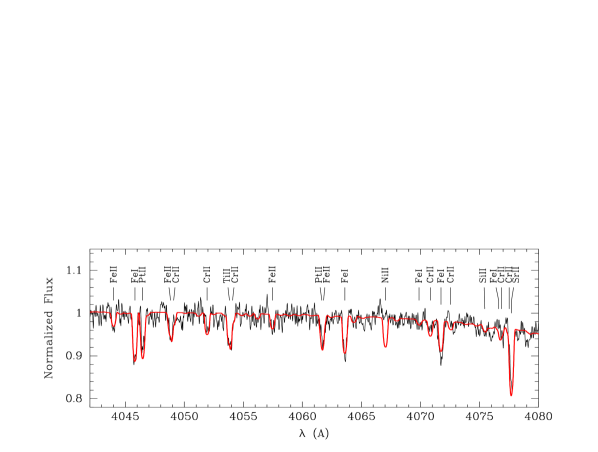
Figure 5: Comparison of the reconstructed spectrum of the star D and the synthetic spectrum (gray line, red in online version) in the spectral region around Pt and Sr lines. In the calculation of this synthetic spectrum, Ni abundance was assumed to be solar so that the large Ni underabundance is better appreciated.

In Fig. 5 we present the synthetic spectrum of star D in the spectral region containing Pt ii 4046, Pt ii 4061, Sr ii 4077, and several Fe and Cr lines. As it is visible in this figure, Ni is underabundant in this star. Fig. 6 shows the synthetic spectra for the regions of the Hg II line at $\lambda 3984$. Even when the rotational broadening is significant, some information about the isotopic composition can be derived from the reconstructed spectra of components C and D. With this aim the line profile was fitted with a synthetic spectrum in which Hg is assumed to be a mixture of the lightest (196) and the heaviest (204) isotopes. As it can be seen in the figure, the best fit suggests that the heaviest isotope is by far the most abundant in both components of the less massive subsystem.

Figure 6: Observed spectra (thin line) and synthetic spectra (heavy line) for stars C and D in the region of the Hg ii line $\lambda$3984 and the Y ii line $\lambda$3982. The isotopic composition for Hg was assumed to be 196=0.9%, 204=99.1% for starC and 196=4%, 204=96% for star D.

5 Discussion

Using high-S/N high-resolution spectra obtained with UVES, we have determined chemical abundance for all four components of the multiple system AO Vel. Further, line profile variations were detected in the spectra of the two most massive stars belonging to the AB system.

Since the multiple system AO Vel is formed by four gravitationally bound stars, we can assume that they have the same original chemical composition and the same age. All components are close to the ZAMS and have already developed different chemical anomalies in their atmospheres, depending on their temperature and probably due to the membership in binary systems. The observed masses and radii for the components of the eclipsing pair suggest that the system age is less than about 40 million years.

The connection between HgMn peculiarity and membership in binary and multiple systems seems to be supported by two observational facts. On the one hand there is a high frequency of binaries and multiples among HgMn stars (Hubrig, Ageorges, & Schöller, 2008). On the other hand, in some binaries the location of chemical spots seems to be related with the position of the binary companion (Hubrig et al., 2006a, see also Savanov et al. 2009). These studies indicates that the presence of a companion can play a significant role in the development and distribution of chemical anomalies on the surface of HgMn stars, probably due to proximity effects on the atmospheric temperature or due to the magnetic field induced in a close binary system. The role that magnetic fields possibly play in the development of anomalies in HgMn stars, which mostly appear in binary systems, has never been critically tested by astrophysical dynamos. Recent magnetohydrodynamical simulations revealed a distinct structure for the magnetic field topology similar to the fractured elemental rings observed on the surface of HgMn stars (see e.g. Fig. 1 in Hubrig, González, & Arlt, 2008). The combination of differential rotation and a poloidal magnetic field was studied numerically by the spherical MHD code of Hollerbach (2000). The presented typical patterns of the velocity and the magnetic field on the surface of the star may as well be an indication for element redistribution on (or in) the star.

Generally He and Si variable Bp stars possess large-scale organized magnetic fields which in many cases appear to occur essentially under the form of a single large dipole located close to the centre of the star. The magnetic field is usually diagnosed through observations of circular polarization in spectral lines. Hubrig et al. (2006b) used the multi-mode instrument FORS 1 mounted on the 8 m Kueyen telescope of the VLT to measure the mean longitudinal magnetic field in the system AO Vel. No detection was achieved with the single low-resolution measurement (R=2000) resulting in $\left<B_{\rm z}\right>$ =  80$\pm$64 G. We should, however, keep in mind that the observed spectropolarimetric spectrum is a composite spectrum consisting of four spectropolarimetric spectra belonging to A, B, C and D components. Each of the companions can possess an individual magnetic field of different geometry, strength and polarity. Since the inhomogeneous elemental distribution of Si and Mg is also observed on the surface of the component B, the presence of a large-scale organized magnetic field is quite possible in this component too. The components C and D show the peculiarity character typical of HgMn stars. Hubrig et al. (2006b) showed that longitudinal magnetic fields in HgMn stars are rather weak, of the order of a few hundred Gauss and less, and the structure of their fields must be sufficiently tangled so that it does not produce a strong net observable circular polarization signature.

Thus, the non-detection of a magnetic field in the system AO Vel can be possibly explained by the dilution of the magnetic signal due to the superposition of four differently polarized spectra. On the other hand, the magnetic field of each component should be detectable with high resolution spectropolarimeters making use of the Zeeman effect in individual metal lines.

The time scale for the peculiarities to be developed remain unclear since the results of studies of evolutionary status of chemically peculiar stars of different type show somewhat contradictory results. The early work by Abt (1979) suggested that the frequency of peculiar stars of Si and HgMn groups increases with age and particularly there exist no peculiar star on the ZAMS. In a more recent photometric search for peculiar stars in five young clusters, Paunzen, Pintado, & Maitzen (2002) also concluded that the CP phenomenon needs at least several Myr to start being effective. On the other hand, some chemically peculiar stars has been detected within very young associations or even in star forming regions like Ori OB1 (Abt & Levato, 1977; Woolf & Lambert, 1999), Lupus 3 (Castelli & Hubrig, 2007), and L988 (Herbig & Dahm, 2006). The results of the present paper show the existence of coeval stars with chemical peculiarities of Si and HgMn types, close to the ZAMS indicating that the age threshold for these peculiarities is similar for both subgroups of chemically peculiar stars. Our study supports the idea that these chemical peculiarities originate quite soon after the star formation.

It is noteworthy, that the subsystem CD, the less massive binary of the AO Vel, shows several similarities with the eclipsing binary AR Aur belonging to the Aur OB1 association. Both systems are formed by stellar components very close to the ZAMS or even in the pre-MS stage (Nordstrom & Johansen, 1994; González et al., 2006), and they have almost the same orbital period, 4^d.13 and 4^d.15 for AR Aur and AO Vel CD, respectively. In both systems the primary is a HgMn star, but while in the AO Vel CD system the secondary companion shares the same peculiarity, in AR Aur the secondary is a normal star (Khokhlova et al., 1995). In fact, the primary component of AR Aur should be compared with star D of the system AO Vel, since they have a similar effective temperature. This similarity in the physical and orbital properties seems to have been translated into the development of similar pattern of chemical abundances: notorious overabundance of Hg and Pt, overabundance of Sr, Y, and Mn at the level of 1–3 dex, slight overabundance of Cr and Ti, and the abundance of Si and Mg close to the solar abundance, or slightly subsolar. We selected a few additional HgMn spectroscopic binaries with effective temperatures close to 11,000 K: HD 32964, HD 89822, HD 173524, and HD 191110. In Fig. 7 the abundances of various elements in AR Aur and selected binaries are compared with those of the AO Vel D companion. The abundances are presented for HgMn stars member of double-lined spectroscopic binaries with periods between 4 and 12 days and having effective temperatures in the range 10 700–11 700 K. For HD 173524 and HD 191110 we plotted the abundances determined in both components. The abundances values have been taken from Adelman (1994), Catanzaro & Leto (2004), and Catanzaro, Leone, & Leto (2003). It is remarkable, how much similar the chemical composition of these stars is. We note, however, that the abundance distribution on the stellar surface of HgMn stars is probably inhomogeneous, and consequently, the chemical composition derived from spectroscopic observations that do not cover the rotational cycle, should be taken just as indicative values until accurate abundance values obtained using Doppler imaging technique become available. The spotted character of magnetic Bp-Ap stars is well known, but also in the case of HgMn stars the presence of chemical spots or belts on the surface is not uncommon (Hubrig, González, & Arlt, 2008; Savanov et al., 2009).

Figure 7: Abundances of the AO Vel D companion (filled squares) compared with published abundances for another seven binary components with similar effective temperatures: HD 32964B (circles), HD 34364A (open squares), HD 89822A (pentagons), HD 173524A (stars), HD 173524B (triangles), HD 191110A (plusses), and HD 191110B (crosses). The dashed line represents the solar abundance.

As already mentioned above, the atmospheric chemical composition of AR Aur exhibits a non-uniform surface distribution with a very interesting pattern related to the position of the companion (Hubrig et al., 2006a). A similar study in AO Vel would be worthwhile to verify whether the elemental distribution on the stellar surfaces of C and D components show a similar behavior. Furthermore, an intensive spectroscopic campaign that would allow the reconstruction of chemical maps for all four components should provide important information for the proper understanding of the origin of chemically peculiar stars.

Appendix A List of spectral lines

Table 5 lists all the spectral lines used for abundance determination. The lines marked with an asterisk are blends. The abundance was determined using the fitting by a synthetic spectrum.

Table 5: Spectral lines used for abundace determination.

ion	$\lambda$(Å)	$\log$ gf	Source	$\log\,N/H$
				A	B	C	D
He I	4026.1844∗	$-$2.625	NIST3	$-$2.3	$-$1.2	$-$2.0	$\leq$$-$3.0
	4026.1859∗	$-$1.448	NIST3
	4026.1860∗	$-$0.701	NIST3
	4026.1968∗	$-$1.449	NIST3
	4026.1983∗	$-$0.972	NIST3
	4026.3570∗	$-$1.324	NIST3
	4387.9291	$-$0.883	NIST3	$--$	$-$1.2	$--$	$--$
	4471.4704∗	$-$2.203	NIST3	$-$3.0	$-$1.25	$-$2.0	$\leq$$-$3.0
	4471.4741∗	$-$1.026	NIST3
	4471.4743∗	$-$0.278	NIST3
	4471.4856∗	$-$1.025	NIST3
	4471.4893∗	$-$0.550	NIST3
	4471.6832∗	$-$0.903	NIST3
	4921.9310	$-$0.435	NIST3	$-$1.8	$-$1.2	$--$	$--$
	5015.6776	$-$0.820	NIST3	$--$	$-$1.0	$--$	$--$
	5875.5987∗	$-$1.516	NIST3	$-$2.7	$-$0.95	$\leq$$-$2.4	$-$2.0
	5875.6139∗	$-$0.341	NIST3
	5875.6148∗	$+$0.408	NIST3
	5875.6251∗	$-$0.340	NIST3
	5875.6403∗	$+$0.137	NIST3
	5875.9663∗	$-$0.215	NIST3
	6678.1517	$+$0.329	NIST3	$-$2.2	$-$0.9	$\leq$$-$3.0	$-$1.8
C II	4267.001∗	$+$0.563	NIST3	$-$4.62	$-$3.87	$-$3.52	$-$3.52
	4267.261∗	$+$0.716	NIST3
	4267.261∗	$-$0.584	NIST3
O I	6155.961∗	$-$1.363	NIST3	$-$3.71	$-$3.56	$-$3.71	$-$3.21
	6155.971∗	$-$1.011	NIST3
	6155.989∗	$-$1.120	NIST3
	6156.737∗	$-$1.487	NIST3	$-$3.71	$-$3.56	$-$3.71	$-$3.21
	6156.755∗	$-$0.898	NIST3
	6156.778∗	$-$0.694	NIST3
	6158.149∗	$-$1.841	NIST3	$-$3.71	$-$3.56	$-$3.71	$-$3.21
	6158.172∗	$-$0.995	NIST3
	6158.187∗	$-$0.409	NIST3
Mg II	4481.126∗	$+$0.749	NIST3	$-$5.5	$-$4.76	$-$4.76	$-$4.96
	4481.150∗	$-$0.553	NIST3
	4481.325∗	$+$0.594	NIST3
Si II	3853.665	$-$1.341	NIST3	$-$4.4	$-$4.3	$-$5.6	$-$5.0
	3856.018	$-$0.406	NIST3	$-$4.4	$-$4.9	$-$5.6	$-$5.0
	3862.595	$-$0.757	NIST3	$-$4.0	$-$4.9	$-$5.6	$-$5.0
	3954.300∗	$-$1.040	KP	$-$3.6	$--$	$--$	$--$
	3954.504∗	$-$0.880	KP
	4128.054	$+$0.359	NIST3	$-$4.1	$-$4.8	$-$4.3	$-$5.2
	4130.872∗	$-$0.783	NIST3	$-$4.1	$-$4.8	$-$4.3	$-$5.0
	4130.894∗	$+$0.552	NIST3
	4187.128∗	$-$1.050	KP	$-$3.7	$--$	$--$	$--$
	4187.128∗	$-$2.590	KP
	4187.151∗	$-$1.160	KP
	4190.724	$-$0.351	LA	$-$3.7	$--$	$--$	$--$
	4198.133	$-$0.611	LA	$-$3.7	$--$	$--$	$--$
	4200.658∗	$-$0.889	NIST3	$-$3.7	$--$	$--$	$--$
	4200.887∗	$-$2.034	NIST3
	4200.898∗	$-$0.733	NIST3
	5041.024	$+$0.029	NIST3	$-$3.8	$-$4.6	$-$3.9	$-$4.5

Table 6: continued

ion	$\lambda$(Å)	$\log$ gf	Source	$\log\,N/N_{H}$
				A	B	C	D
	5055.984∗	$+$0.523	NIST3	$-$4.0	$-$4.7	$-$4.3	$-$4.8
	5056.317∗	$-$0.492	NIST3
	5185.232∗	$+$0.472	LA	$-$3.8	$--$	$--$	$--$
	5185.520∗	$-$1.603	NIST3
	5185.520∗	$-$0.302	NIST3
	5185.555∗	$-$0.456	NIST3
	5688.817	$+$0.126	NIST3	$-$3.6	$--$	$--$	$--$
	5701.370	$-$0.057	NIST3	$-$3.6	$--$	$--$	$--$
	5957.559	$-$0.225	NIST3	$-$4.0	$-$4.9	$-$4.6	$-$4.8
	5978.930	$+$0.084	NIST3	$-$4.0	$-$5.4	$-$4.6	$-$4.8
	6347.103	$+$0.149	NIST3	$-$3.6	$-$4.4	$-$4.0	$-$4.6
	6371.371	$-$0.082	NIST3	$-$3.7	$-$4.5	$-$4.3	$-$4.6
P II	4178.463	$-$0.409	HI	$-$6.59	$--$	$--$	$--$
	6024.178	$+$0.137	NIST3	$-$5.39	$--$	$--$	$--$
	6034.039	$-$0.220	NIST3	$-$5.39	$--$	$--$	$--$
	6043.084	$+$0.416	NIST3	$-$5.39	$--$	$--$	$--$
S II	4153.068	$+$0.617	NIST3	$-$4.71	$-$4.71	$-$4.71	$-$4.71
	5027.203	$-$0.705	NIST3	$-$4.71	$-$4.71	$-$4.71	$-$4.71
Ti II	4399.765	$-$1.190	PTP	$\leq$$-$7.5	$\leq$$-$8.0	$-$7.02	$--$
	4411.072	$-$0.670	PTP	$\leq$$-$7.5	$\leq$$-$8.0	$-$7.02	$-$6.37
	4418.714	$-$1.970	PTP	$\leq$$-$7.5	$\leq$$-$8.0	$-$7.02	$-$6.37
	4468.492	$-$0.620	NIST3	$\leq$$-$7.5	$\leq$$-$8.0	$-$7.02	$-$6.37
Cr II	4261.913	$-$1.531	K03Cr	$--$	$--$	$-$6.37	$-$5.87
	5237.329	$-$1.160	NIST3	$--$	$--$	$-$6.37	$-$5.87
	5313.590	$-$1.650	NIST3	$--$	$--$	$-$6.37	$-$5.87
Mn II	4206.367	$-$1.590	K03Mn	$--$	$--$	$-$5.65	$-$5.65
	4478.635	$-$0.942	K03Mn	$--$	$--$	$-$5.65	$-$5.65
Fe II	4178.862	$-$2.440	FW06	$-$5.75	$-$5.0	$--$	$--$
	4233.172	$-$1.809	FW06	$--$	$--$	$-$4.24	$-$4.54
	4303.176	$-$2.610	FW06	$-$5.75	$-$5.0	$--$	$--$
	4385.387	$-$2.580	FW06	$-$5.75	$-$5.0:	$--$	$--$
	4416.830	$-$2.600	FW06	$-$5.75	$-$5.0	$-$3.50	$-$4.14
	4923.927	$-$1.210	FW06	$-$5.75	$-$5.3	$-$4.24	$-$4.85
	5018.440	$-$1.350	FW06	$-$4.90	$-$4.8	$-$4.00	$-$4.54
	5100.607∗	$+$0.144	K09	$--$	$--$	$-$4.24	$-$4.54
	5100.734∗	$+$0.671	J07
	5169.033	$-$0.870	FW06	$-$5.20	$-$4.8	$-$4.24	$-$4.54
	5197.577	$-$2.054	FW06	$--$	$--$	$-$4.34	$-$4.70
	5227.483	$+$0.831	J07	$--$	$--$	$-$4.24	$-$4.54
	5234.625	$-$2.210	FW06	$--$	$--$	$-$4.34	$-$4.54
	5276.002	$-$1.900	FW06	$-$4.8	$-$5.8	$-$4.54	$-$4.74
	5316.615	$-$1.780	FW06	$-$4.8	$-$5.0	$-$4.34	$-$4.74
	5362.741∗	$-$0.708	K09	$--$	$--$	$-$4.00	$-$4.34
	5362.869∗	$-$2.855	K09
	5362.967∗	$+$0.008	K09
Ni II	4015.474	$-$2.410	K03Ni	$--$	$--$	$--$	$\leq$$-$6.79
	4067.031	$-$1.834	K03Ni	$--$	$--$	$--$	$\leq$$-$6.79
Sr II	4077.709	$+$0.151	NIST3	$--$	$--$	$--$	$-$8.27

Table 7: continued

ion	$\lambda$(Å)	$\log$ gf	Source	$\log\,N/N_{H}$
				A	B	C	D
Y II	3982.592	$-$0.493	NIST3	$--$	$--$	$--$	$-$7.45
	4235.727	$-$1.509	NIST3	$--$	$--$	$--$	$-$6.60
	4309.620	$-$0.745	NIST3	$--$	$--$	$--$	$-$6.95
	4883.684	$+$0.071	NIST3	$--$	$--$	$--$	$-$7.25
	4900.120	$-$0.090	NIST3	$--$	$--$	$--$	$-$7.25
	5200.406	$-$0.579	NIST3	$--$	$--$	$--$	$-$7.45
	5205.722	$-$0.342	NIST3	$--$	$--$	$--$	$-$7.15
Pt II	4046.443	$-$1.190	ENG	$--$	$--$	$--$	$-$5.94
	4061.644	$-$1.890	ENG	$--$	$--$	$--$	$-$5.94
	4288.371	$-$1.570	ENG	$--$	$--$	$--$	$-$5.94:
Hg II	3983.890	$-$1.510	NIST3	$--$	$--$	$--$	$-$6.55

NIST3: NIST atomic spectra Database, version 3 at http://physics.nist.gov;

FW06 : Fuhr & Wiese (2006)

PTP: Pickering, Thorne, & Perez (2002)

LA : Lanz & Artru (1985)

KP : Kurucz & Peytremann (1975)

HI : Hibbert (1988)

J07: Johannson (2007), private communication

K03Cr:Kurucz (2003), http://kurucz.harvard.edu/atoms/2401/gf2401.pos

K03Mn:Kurucz (2003), http://kurucz.harvard.edu/atoms/2501/gf2501.pos

K03Ni:Kurucz (2003), http://kurucz.harvard.edu/atoms/2801/gf2801.pos

K09: Kurucz (2009), http://kurucz.harvard.edu/atoms/2601/gf2601.pos

We thank to Charles R. Cowley and Rainer Arlt for helpful discussions.

References

- Abt (1979) Abt H. A., 1979, ApJ, 230, 485
- Abt & Levato (1977) Abt H. A., Levato H., 1977, PASP, 89, 797
- Adelman (1994) Adelman S. J., 1994, MNRAS, 266, 97
- Bidelman & MacConnell (1973) Bidelman W. P., MacConnell D. J., 1973, AJ, 78, 687
- Castelli & Hubrig (2007) Castelli F., Hubrig S., 2007, A&A, 475, 1041
- Catanzaro & Leto (2004) Catanzaro G., Leto P., 2004, A&A, 416, 661
- Catanzaro, Leone, & Leto (2003) Catanzaro G., Leon, F., Leto P., 2003, A&A, 407, 669
- Clausen et al. (1995) Clausen J. V., Giménez A., van Houten C. J., 1995, A&AS, 109, 425
- Fuhr & Wiese (2006) Fuhr, J. R., & Wiese, W. L. 2006, Journal of Physical and Chemical Reference Data, 3 5, 1669
- González & Levato (2006) González J. F., Levato H., 2006, A&A, 448, 283
- González et al. (2006) González J. F., Hubrig S., Nesvacil N., North P., 2006, A&AS, 449, 327
- González, Nesvacil, & Hubrig (2008) González J. F., Nesvacil N., Hubrig S., 2008, in Santos N. C., Pasquini L., Correia A. C. M., Romanielleo M., eds, Precision Spectroscopy in Astrophysics. Springer-Verlag, Berlin, p. 291
- Grevesse & Sauval (1998) Grevesse N., Sauval A. J., 1998, Space Science Reviews, 85, 161
- Herbig & Dahm (2006) Herbig G. H., Dahm S. E., 2006, AJ, 131, 1530
- Hensberge et al. (2004) Hensberge H., Nitschelm C., Freyhammer L. M., et al., 2004, ASP Conf. Ser., 318, 309
- Hibbert (1988) Hibbert, A., 1988, Physica Scripta 38, 37
- Hollerbach (2000) Hollerbach R., 2000, Int. J. Numer. Meth. Fluids, 32, 773
- Hubrig et al. (2006b) Hubrig S., North P., Schöller M., Mathys G., 2006b, AN, 327, 289
- Hubrig et al. (2006a) Hubrig S., González J. F., Savanov I., Schöller M., Ageorges N., Cowley C. R., Wolff B., 2006a, MNRAS, 371, 1953
- Hubrig, Ageorges, & Schöller (2008) Hubrig S., Ageorges N., Schöller M., 2008, in Hubrig S., Petr-Gotzens M., Tokovinin A., eds, Multiple Stars Across the H-R Diagram, ESO Astrophysics Symposia. Springer-Verlag, Berlin, p. 155
- Hubrig, González, & Arlt (2008) Hubrig S., González J. F., Arlt R., 2008, Contr. Ast. Obs. Skalnaté Pleso, 38, 415
- Khokhlova et al. (1995) Khokhlova V. L., Zverko Y., Zhizhnovskii I., Griffin R. E. M., 1995, AstL, 21, 818
- Kurucz & Peytremann (1975) Kurucz, R. .L., & Peytremann, E., 1975, SAO Special Report, 362
- Kurucz (1993) Kurucz R. L., 1993, CDROM13, SAO Cambridge
- Kuschnig et al. (1999) Kuschnig R., Ryabchikova T. A., Piskunov N. E., Weiss W. W., Gelbmann M. J., 1999, A&A, 348, 924
- Lanz & Artru (1985) Lanz, T., & Artru, M. .C., 1985, Physica Scripta, 32, 115
- Lejeune & Schaerer (2001) Lejeune T., Schaerer D., 2001, A&A, 366, 538
- Leone et al. (1997) Leone F., Catalano F. A., Malaroda S., 1997, A&A, 325, 1125
- Nordstrom & Johansen (1994) Nordstrom B., Johansen K. T., 1994, A&A, 282, 787
- North & Debernardi (2004) North P., Debernardi Y. 2004 ASPC, 318, 297
- Paunzen, Pintado, & Maitzen (2002) Paunzen E., Pintado O. I., Maitzen H. M., 2002, A&A, 395, 823
- Pickering, Thorne, & Perez (2002) Pickering J. C., Thorne A. P., Perez R., 2002, ApJS, 138, 247
- Savanov et al. (2009) Savanov I. S., Hubrig S., González J. F., Schöller M., 2009, IAUS 259, 401
- Woolf & Lambert (1999) Woolf V. M., Lambert D. L., 1999, ApJ, 520L, 55