Abstract

It is shown that the Quark-Level Linear $\sigma$ Model (QLL$\sigma$M) leads to a prediction for the diamagnetic term of the polarizabilities of the nucleon which is in excellent agreement with experimental data. The bare mass of the $\sigma$ meson is predicted to be $m_{\sigma}=666$ MeV and the two-photon width $\Gamma(\sigma\to\gamma\gamma)=(2.6\pm 0.3)$ keV. It is argued that the mass predicted by the QLL$\sigma$M corresponds to the $\gamma\gamma\to\sigma\to N\bar{N}$ reaction, i.e. to a $t$-channel pole of the $\gamma N\to N\gamma$ reaction. Large-angle Compton scattering experiments revealing effects of the $\sigma$ meson in the differential cross section are discussed. Arguments are presented that these findings may be understood as an observation of the Higgs boson of strong interaction while being a part of the constituent quark.

1 Introduction

The $\sigma$ meson introduced by Schwinger [1] and Gell-Mann–Levy [2] has attracted great interest because there are good reasons to consider it as the Higgs boson of strong interaction, an aspect which recently has been emphasized by several authors [4, 3, 5, 6]. The mass of the $\sigma$ meson is predicted by the Quark-Level Linear $\sigma$ Model (QLL$\sigma$M) [7] (see also [8, 9] and references therein) to be $m_{\sigma}=666$ MeV, whereas $\pi$-$\pi$ scattering analyses led to $\sqrt{s_{\sigma}}=M_{\sigma}-i\,\Gamma_{\sigma}/2$ with $M_{\sigma}=441^{+16}_{-8}$ MeV and $\Gamma_{\sigma}=544^{+18}_{-25}$ MeV in one recent evaluation (CCL)[10], or $\sqrt{s_{\sigma}}=(476-628)-i(226-346)$ MeV when tests of the stability of fits to data are taken into account [11]. It certainly is extremely important to understand how these two masses are related to each other. The finding is that $m_{\sigma}=666$ MeV is the bare mass of the $\sigma$ meson which is observed in space-like Compton scattering $\gamma\gamma\to\sigma\to N\bar{N}$, i.e. as a $t$-channel pole of Compton scattering $\gamma N\to N\gamma$. For the electromagnetic polarizabilities space-like Compton scattering is equally important as time-like Compton scattering $\gamma N\to N\gamma$ ($s$-channel). The $\sigma$ and non-$\sigma$ components of the electromagnetic polarizabilities for the proton $(p)$ and the neutron $(n)$ are $\alpha_{p,n}(\sigma)=-\beta_{p,n}=7.6$, $\alpha_{p}({\rm non-}\sigma)=4.4$, $\beta_{p}({\rm non-}\sigma)=9.5$, $\alpha_{n}({\rm non-}\sigma)=5.8$, $\beta_{n}({\rm non-}\sigma)=9.4$ in units of $10^{-4}$ fm³. On the quark level the reaction $\gamma\gamma\to\sigma\to N\bar{N}$ implies that two photons with parallel planes of linear polarization interact with $\sigma$ mesons, being parts of the constituent quarks. In this sense it is justified to consider space-like Compton scattering as an in-situ observation of the Higgs boson of strong interaction.

In addition to the specific aspects of the $\sigma$ meson as outlined in the preceding paragraph this particle is of interest because it has been observed as an intermediate state in many reactions [12]. Therefore, there is no doubt that this particle exists and that it belongs to a scalar nonet ($\sigma(600)$, $f_{0}(980)$, $a_{0}(980)$, $\kappa(800)$) below 1 GeV. A problem may appear due to the fact that there is also a scalar nonet above 1 GeV. This has led to the assumption that the scalar nonet above 1 GeV should be understood as $q\bar{q}$ states whereas the scalar nonet below 1 GeV should be understood as $qq\bar{q}\bar{q}$ states (see e.g. [4] and references therein). Other versions consider meson molecules and gluonic components (see [3, 4, 5, 6, 13, 14, 15, 16] and references therein). It is hard to see that strict criteria can be found giving proof of the validity of one model and excluding the validity of an other. The best way to proceed is to start with a model for the low-mass scalar mesons where $q\bar{q}$ is a ${}^{3}P_{0}$ core state which may couple to other hadronic or gluonic configurations [15]. Then the essential properties as e.g. the two-photon width $\Gamma(\sigma\to\gamma\gamma)$ may be understood in terms of the $q\bar{q}$ core whereas other components may show up in hadronic reactions where scalar mesons appear as intermediate states.

The present work is a continuation of a systematic series of studies [8, 17, 18, 19, 20] on the electromagnetic structure of the nucleon, following experimental work on Compton scattering and a comprehensive review on this topic [21]. These recent investigations have shown [8, 17, 18, 19, 20] that a systematic study of all partial resonant and nonresonant photo-excitation processes of the nucleon and of their relevance for the fundamental structure constants of the nucleon as there are the electric polarizability ($\alpha$), the magnetic polarizability ($\beta$) and the backward spin-polarizability ($\gamma_{\pi}$) is essential for an understanding of the electromagnetic structure of the nucleon. In addition it has been found that the structure of the constituent quarks and their coupling to pseudoscalar and scalar mesons is important for the understanding of the electric and magnetic polarizabilities and of the backward spin-polarizability. The main purpose of the present work is to prove that the method of calculating the $t$-channel contribution from the reaction $\gamma\gamma\to\sigma\to N\bar{N}$ where the properties of the $\sigma$ meson are taken from the QLL$\sigma$M is a precise procedure and largely superior to previous approaches where the combination of the two reactions $\gamma\gamma\to\sigma\to\pi\pi$ and $\gamma\gamma\to\sigma\to N\bar{N}$ is exploited.

2 The dynamical linear $\sigma$ model on the quark level and the mass of the $\sigma$-meson

In the following we give a résumé of the dynamical linear $\sigma$ model on the quark level [7] which in short term may be named Quark-Level Linear $\sigma$ Model (QLL$\sigma$M) [9].

The Lagrangian of the Nambu–Jona-Lasinio (NJL) model has been formulated in two equivalent ways [22, 23, 24, 25]

$${\cal L}_{\rm NJL}=\bar{\psi}(i\mbox{$/\!\!\!\partial$}-m_{0})\psi+\frac{G}{2}[(\bar{\psi}\psi)^{2}+(\bar{\psi}i\gamma_{5}\mbox{\boldmath$\tau$}\psi)^{2}],$$ (1)

$${\rm and}\hskip 28.45274pt$$ (2)

$${\cal L^{\prime}}_{\rm NJL}=\bar{\psi}i\mbox{$/\!\!\!\partial$}\psi-g\bar{\psi}(\sigma+i\gamma_{5}\mbox{\boldmath$\tau$}\cdot\mbox{\boldmath$\pi$})\psi-\frac{1}{2}\delta\mu^{2}(\sigma^{2}+\mbox{\boldmath$\pi$}^{2})+\frac{gm_{0}}{G}\sigma,$$

$${\rm where}\hskip 28.45274pt$$ (3)

$$G=g^{2}/\delta\mu^{2}\quad\mbox{and}\quad\delta\mu^{2}=(m^{\rm cl}_{\sigma})^{2}.$$

Eq. (1) describes the four-fermion version of the NJL model and Eq. (2) the bosonized version. The quantity $m_{0}=(m_{u}+m_{d})/2$ denotes the average current quark mass for two flavors, $\psi$ the spinor of constituent quarks with two flavors. The quantity $G$ is the coupling constant of the four-fermion version, $g$ the Yukawa coupling constant and $\delta\mu$ a mass parameter entering into the mass counter-term of Eq. (2). The coupling constants $G$, $g$ and the mass parameter $\delta\mu$ are related to each other and to the $\sigma$ meson mass in the chiral limit (cl), $m^{\rm cl}_{\sigma}$, as given in (3). The relation $\delta\mu^{2}=(m^{\rm cl}_{\sigma})^{2}$ can easily be derived by applying spontaneous symmetry breaking to $\delta\mu$ in analogy to spontaneous symmetry breaking predicted by the linear $\sigma$ model (L$\sigma$M) for the mass parameter $\mu$ entering into that model [26].

Using diagrammatic techniques the following equations may be found [7, 25, 27]

$$M^{*}=m_{0}+8\,i\,GN_{c}\int^{\Lambda}\frac{d^{4}p}{(2\pi)^{4}}\frac{M^{*}}{p^{2}-M^{*2}},\quad M=-\frac{8iN_{c}g^{2}}{(m^{\rm cl}_{\sigma})^{2}}\int\frac{d^{4}p}{(2\pi)^{4}}\frac{M}{p^{2}-M^{2}},$$ (4)

$$f^{2}_{\pi}=-4\,i\,N_{c}M^{*2}\int^{\Lambda}\frac{d^{4}p}{(2\pi)^{4}}\frac{1}{(p^{2}-M^{*2})^{2}},\quad f^{\rm cl}_{\pi}=-4iN_{c}gM\int\frac{d^{4}p}{(2\pi)^{4}}\frac{1}{(p^{2}-M^{2})^{2}},$$ (5)

$$m^{2}_{\pi}=-\frac{m_{0}}{M^{*}}\frac{1}{4\,i\,GN_{c}I(m^{2}_{\pi})},$$ (6)

$$I(k^{2})=\int^{\Lambda}\frac{d^{4}p}{(2\pi)^{4}}\frac{1}{[(p+\frac{1}{2}k)^{2}-M^{*2}][(p-\frac{1}{2}k)^{2}-M^{*2}]}.$$

The expression given on the l.h.s. of (4) is the gap equation with $M^{*}$ being the mass of the constituent quark with the contribution $m_{0}$ of the current quarks included and $N_{c}=3$ being the number of colors. The quantity $M$ on the r.h.s. of Eq. (4) is the mass of the constituent quark in the chiral limit. The l.h.s. of Eq. (5) represents an expression for the pion decay constant having the experimental value $f_{\pi}=(92.42\pm 0.26)$ MeV [12]. On the r.h.s. of Eq. (5) the corresponding expression for $f^{\rm cl}_{\pi}$ is given which is the same quantity in the chiral limit. The relation for the pion mass in Eq. (6) has no counterpart in the chiral limit because there the pion mass is zero.

In principle the gap parameter $M^{*}$ and through this the mass of the $\sigma$ meson $m_{\sigma}$ can be determined using the l.h.s. relations of Eqs. (4) to (6). This has been carried out in [27] leading to $m_{\sigma}\approx 2M^{*}\approx 668$ MeV.

A more elegant way to predict $m_{\sigma}$ on an absolute scale introduced by Delbourgo and Scadron [7] is obtained by exploiting the r.h.s. of Eqs. (4) and (5). Making use of the identity (dimensional regularization [28, 7])

$$-i\frac{(m^{\rm cl}_{\sigma})^{2}}{16N_{c}g^{2}}=\int\frac{d^{4}p}{(2\pi)^{4}}\left[\frac{M^{2}}{(p^{2}-M^{2})^{2}}-\frac{1}{p^{2}-M^{2}}\right]=-\frac{iM^{2}}{(4\pi)^{2}}$$ (7)

we arrive at

$$(m^{\rm cl}_{\sigma})^{2}=\frac{N_{c}g^{2}M^{2}}{\pi^{2}},$$ (8)

and with $m^{\rm cl}_{\sigma}=2M$ at the Delbourgo-Scadron relation [7]

$$g=g_{\pi qq}=g_{\sigma qq}=2\pi/\sqrt{N_{c}}=3.63.$$ (9)

The $\sigma$-meson mass corresponding to this coupling constant is

$$m_{\sigma}=666.0\,\,\,{\rm MeV},$$ (10)

where use has been made of $m^{2}_{\sigma}=(m^{\rm cl}_{\sigma})^{2}+{\hat{m}}^{2}_{\pi}$, $f^{\rm cl}_{\pi}=89.8$ MeV [31], $M=325.8$ MeV and ${\hat{m}}_{\pi}=138.0$ MeV. This result may also be compared with information from magnetic moments.

It has to be noted that the present version of the QLL$\sigma$M is incomplete in the sense that the coupling of the $\sigma$ meson to meson loops is not taken into account. These meson loops lead to contributions to the two-photon decay width $\Gamma(\sigma\to\gamma\gamma)$ of the $\sigma$ meson in addition to the dominant $q\bar{q}$ contribution (see [9] and Table 1).

3 The two-photon decay width of the $\sigma$ meson

In the quark model the $\sigma$ meson has the structure

$$|n\bar{n}\rangle=\frac{1}{\sqrt{2}}|u\bar{u}+d\bar{d}\rangle.$$ (11)

Then the principal contributions to the amplitude ${\cal M}(\sigma\to\gamma\gamma)$ comes from the up and down quark triangle diagrams [9], yielding (with $N_{c}=3$)

$${\cal M}(\sigma\to\gamma\gamma)=\frac{5\alpha_{e}}{3\pi f_{\pi}}V_{q}(\xi),$$ (12)

$$V_{q}(\xi)=2\xi[2+(1-4\xi)I(\xi)],$$ (13)

where $\alpha_{e}=e^{2}/4\pi=1/137.04$, $\xi={\hat{m}}^{2}_{q}/m^{2}_{\sigma}$ and $I(\xi)$ is the triangle loop integral given by

$$I(\xi)\begin{cases}=\frac{\pi^{2}}{2}-2\log^{2}\left[\sqrt{\frac{1}{4\xi}}+\sqrt{\frac{1}{4\xi}-1}\right]+2\pi\,i\,\log\left[\sqrt{\frac{1}{4\xi}}+\sqrt{\frac{1}{4\xi}-1}\right]\,\,\,(\xi\leq 0.25),\\ =2\arcsin^{2}\left[\sqrt{\frac{1}{4\xi}}\right]\,\,\,(\xi\geq 0.25).\end{cases}$$ (14)

With the average constituent quark mass ${\hat{m}}_{q}=330$ MeV and $m_{\sigma}=666$ MeV we arrive at a correction factor of $V_{q}(\xi)=1.025$, whereas in the chiral limit, ${\hat{m}}_{q}\to M$ and $m_{\sigma}\to 2M$, we have $V_{q}(\xi)=1.0$. We see that the possible correction due to the factor $V_{q}(\xi)$ is small and may be disregarded in view of possible other uncertainties. Then with $V_{q}(\xi)=1$ and

$$\Gamma(\sigma\to\gamma\gamma)=\frac{m^{3}_{\sigma}}{64\pi}|{\cal M}(\sigma\to\gamma\gamma)|^{2}$$ (15)

we arrive at

$$\Gamma(\sigma\to\gamma\gamma)=(2.6\pm 0.3)\,\,\,\text{keV}.$$ (16)

The value for the two-photon decay width given in (16) leads to an excellent agreement with the experimental electromagnetic polarizabilities of the nucleon and, therefore, is experimentally confirmed through this agreement. This is especially true for the electric polarizability $\alpha_{p}$ of the proton which has the smallest experimental error, viz. $\Delta\alpha_{p}/\alpha_{p}\approx 5\%$. Using $\Delta\Gamma(\sigma\to\gamma\gamma)/\Gamma(\sigma\to\gamma\gamma)\approx 2\Delta\alpha_{p}/\alpha_{p}\approx 10\%$ the error given in (16) is obtained (see Table 2 for details).

4 Properties of the reaction $\gamma\gamma\to\sigma\to N{\bar{N}}$

Let us first discuss the kinematics of Compton scattering. The conservation of energy and momentum in nucleon Compton scattering

$$\gamma(k,\lambda)+N(p)\to\gamma^{\prime}(k^{\prime},\lambda^{\prime})+N^{\prime}(p)$$ (17)

is given by

$$k+p=k^{\prime}+p^{\prime}$$ (18)

where $k$ and $k^{\prime}$ are the 4-momenta of the incoming and outgoing photon, $\lambda$ and $\lambda^{\prime}$ the respective helicities and $p$ and $p^{\prime}$ the 4-momenta of the incoming and outgoing nucleon. Mandelstam variables are introduced through the relations

$$s=(k+p)^{2}=(k^{\prime}+p^{\prime})^{2},$$ (19)

$$t=(k-k^{\prime})^{2}=(p^{\prime}-p)^{2},$$ (20)

$$u=(k-p^{\prime})^{2}=(k^{\prime}-p)^{2},$$ (21)

$$s+t+u=2m^{2},$$ (22)

where $m$ is the mass of the nucleon. At negative $t$ this quantity can be interpreted in terms of the c.m. scattering angle $\theta_{s}$:

$$\sin^{2}\frac{\theta_{s}}{2}=-\frac{st}{(s-m^{2})^{2}}.$$ (23)

Compton scattering may be described by invariant amplitudes $A_{i}(s,t)$ $(i=1-6)$ which are analytic functions in the two variables $s$ and $t$ and, therefore, may be treated in terms of dispersion relations. The third variable $u$ is not taken into account because of the constraint given in (22). The degrees of freedom of the nucleon including the structure of the constituent quarks enter into the invariant amplitudes via a cut on the real axis of the complex $s$-plane and in terms of pointlike singularities on the positive real axis of the $t$-plane. The $s$-channel cut contains the total photoabsorption cross section and through a decomposition in terms of excitation mechanisms the complete electromagnetic structure of the nucleon as seen in one-photon processes. The pointlike singularities on the positive real $t$-axis may be related to the structure of the constituent quarks which couple to all mesons with a nonzero meson-quark coupling constant. Of these the $\pi^{0}$ and the $\sigma$ meson are of special interest. On the one hand they couple to two photons with perpendicular and parallel planes of linear polarization, respectively, and on the other hand they enter into the QLL$\sigma$M as described in Section 2. In a formal sense the singularities on the positive real $t$-axis correspond to the fusion of two photons with 4-momenta $k_{1}$ and $k_{2}$ and helicities $\lambda_{1}$ and $\lambda_{2}$ to form a $t$-channel intermediate state $|\pi^{0}\rangle$ or $|\sigma\rangle$ from which – in a second step – a proton-antiproton pair is created. The corresponding reaction may be formulated in the form

$$\gamma(k_{1},\lambda_{1})+\gamma(k_{2},\lambda_{2})\to\bar{N}(p_{1})+N(p_{2}).$$ (24)

In the present case the $N\bar{N}$ pair creation-process is virtual, i.e. the energy is too low to put the proton-antiproton pair on the mass shell. In the c.m. system the 3-momenta of the two photons are related by ${\bf k_{1}}+{\bf k_{2}}=0$, leading to $t=(\omega_{1}+\omega_{2})^{2}=(W^{t})^{2}$ where $W^{t}$ is the total energy.

The $\pi^{0}$ singularity enters into the invariant amplitude $A_{2}$ and the $\sigma$ singularity into the invariant amplitude $A_{1}$ [29]. Let us first discuss the well known case of the $\pi^{0}$ pole contribution. The fixed $\theta=\pi$ dispersion relation is

$${\tilde{A}}_{2}^{\pi^{0}}(s,t)=\frac{1}{\pi}\int^{\infty}_{t_{0}}{\rm Im}_{t}{\tilde{A}}_{2}(s^{\prime},t^{\prime})\frac{dt^{\prime}}{t^{\prime}-t-i0}$$ (25)

with the solution for a pointlike singularity [30, 21]

$${\tilde{A}}^{\pi^{0}}_{2}(t)=\frac{{\cal M}(\pi^{0}\to\gamma\gamma)\,g_{\pi NN}}{t-m^{2}_{\pi^{0}}}\mbox{\boldmath$\tau$}_{3}.$$ (26)

The analogous formula for the $\sigma$ meson is

$${\tilde{A}}^{\sigma}_{1}(t)=\frac{{\cal M}(\sigma\to\gamma\gamma)\,g_{\sigma NN}}{t-m^{2}_{\sigma}}.$$ (27)

The relation given in (26) is valid in the whole complex $t$-plane especially also in the physical range of the Compton scattering process at $\theta=\pi$ where kinematical constraints are absent. For (27) the same is true provided the intermediate state in the reaction $\gamma\gamma\to\sigma\to N\bar{N}$ has a definite mass of $m_{\sigma}=666$ MeV as conjectured here. The observation that the predicted mass $m_{\sigma}=666$ MeV together with the predicted two-photon width $\Gamma(\sigma\to\gamma\gamma)=2.6$ keV obtained for the $\sigma=\frac{1}{\sqrt{2}}(u\bar{u}+d\bar{d})$ configuration is in perfect agreement with the experimental electromagnetic polarizabilities is one of the main achievements of the present and our related previous works, thus supporting our supposition that this description of the $\sigma$ meson pole contribution is correct.

4.1 Analysis of the $\gamma\gamma\to\sigma\to\pi\pi$ reaction

Table 1 summarizes the results available for the two-photon width $\Gamma(\sigma\to\gamma\gamma)$ obtained from the most recent analyses of the $\gamma\gamma\to\sigma\to\pi\pi$ reactions. For comparison we also give the present result obtained from the QLL$\sigma$M model including the $q\bar{q}$ component only and the full calculation of [9] where also meson loops are included. From the large number of very different results recently published for the $\gamma\gamma\to\sigma\to\pi\pi$ reaction it is difficult to decide whether $2.6$ or $3.5$ given in lines 3 and 4 of Table 1 are in better agreement with the $\gamma\gamma\to\sigma\to\pi\pi$ data. However, we should keep in mind that the result ($2.6\pm 0.3$) keV is supported by the experimental electric polarizability $\alpha_{p}$ (see Table 2).

Table 1: Two-photon width of the $\sigma$ meson from the $\gamma\gamma\to\pi\pi$ reaction compared with the QLL$\sigma$M. In line 3 the $q\bar{q}$ contribution and information obtained from the electric polarizability $\alpha_{p}$ of the proton is taken into account. In line 4 the full calculation including meson loops is taken into account.

$\Gamma(\sigma\to\gamma\gamma)$	method	reference
$[{\rm keV}]$	$[{\rm MeV}]$
$2.6\pm 0.3$	QLL$\sigma$M $q\bar{q}$ and $\alpha_{p}$	present
$3.5$	QLL$\sigma$M $q\bar{q}$ and meson loops	[9]
$4.1\pm 0.3$	$\gamma\gamma\to\pi^{0}\pi^{0}$	[13] (result 1)
$1.8\pm 0.4$	$\gamma\gamma\to\pi^{0}\pi^{0}$	[32] (result 2)
$2.1\pm 0.3$	$\gamma\gamma\to\pi^{0}\pi^{0}$	[32] (result 3)
$3.0\pm 0.3$	$\gamma\gamma\to\pi^{0}\pi^{0}$	[32] (result 4)
$1.68\pm 0.15$	$\gamma\gamma\to\pi^{0}\pi^{0}$	[33] (result 5)
$3.9\pm 0.6$	$\gamma\gamma\to\pi^{0}\pi^{0},\pi^{+}\pi^{-}$	[34] (result 6)
$3.1\pm 0.5$	$\gamma\gamma\to\pi^{+}\pi^{-}$	[35] (result 7)
$2.4\pm 0.4$	$\gamma\gamma\to\pi^{+}\pi^{-}$	[35] (result 8)
$2.3\pm 0.4$	average of the results $(1-8)$

The weighted average of the results 1–8 is $\Gamma(\sigma\to\gamma\gamma)=(2.3\pm 0.4)$ keV and thus consistent with the present result and also consistent with the result of [9]. We consider this general agreement as quite satisfactory.

4.2 Properties of the reaction $\gamma\gamma\to\sigma\to N\bar{N}$ and the $t$-channel part of the polarizability difference $(\alpha-\beta)^{t}$

The pole at $\sqrt{s_{\sigma}}=666$ MeV has gained importance because it provides an easy access to the calculation of the $t$-channel part of Compton scattering as given by the process $\gamma\gamma\to\sigma\to N\bar{N}$. This is illustrated in Figure 1. In a) and b) the $t$-channel pole contributions corresponding to the $\pi^{0}$ and $\sigma$ meson are compared with each other. These two poles differ by their locations at $m_{\pi^{0}}=135.0$ MeV and $m_{\sigma}=666$ MeV, respectively, and their two-photon widths. In addition they differ by the fact that the pseudoscalar meson couples to two photons with perpendicular planes of

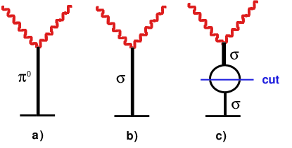
Figure 1: $\pi^{0}$ and $\sigma$ pole graphs.

linear polarization whereas the scalar meson couples to two photons with parallel planes of linear polarization. Except for this there are no further differences in the two $t$-channel contributions. The $\sigma$ meson pole contribution was originally used in [29] in connection with the prediction of differential cross sections for Compton scattering. Its relation to the QLL$\sigma$M was first described in [8]. Prior to this discovery [8] the calculation of the scalar $t$-channel contribution to nucleon Compton scattering had to rely on the available information on the two reactions $\gamma\to\sigma\to\pi\pi$ and $\pi\pi\to\sigma\to N\bar{N}$ where the $\sigma$ meson was taken into account through the $\pi\pi$ phase relation. This corresponds to the graph c) in Figure 1. Here the $\sigma$ propagator has to be cut into two pieces for the purpose of the calculation. This procedure has also been applied by BEFT [36] to make predictions for the $t$-channel contribution of the difference $(\alpha-\beta)^{t}$ of the electric and magnetic polarizability.

In more detail the procedures of calculating $(\alpha-\beta)^{t}$ from the graphs b) and c) in Figure 1 are given in Eqs. (28) and (29), respectively. Using the $\gamma\gamma\to\sigma\to N{\bar{N}}$ reaction the result

$$(\alpha-\beta)^{t}=\frac{{\cal M}(\sigma\to\gamma\gamma)\,g_{\sigma NN}}{2\pi\,m^{2}_{\sigma}}=15.2$$ (28)

(in units of 10^-4fm³) is obtained when inserting ${\cal M}(\sigma\to\gamma\gamma)=(5\alpha_{e})/(3\pi f_{\pi})$, $m_{\sigma}=666$ MeV and $g_{\sigma NN}=13.169\pm 0.057$ [37]. In case of graph c) in Figure 1 we restrict ourselves in the calculation of the $t$-channel absorptive part to intermediate states with two pions with angular momentum $J\leq 2$. Then the $t$-channel part of the BEFT sum rule [36] takes the form:

$$(\alpha-\beta)^{t} = \frac{1}{16\pi^{2}}\int^{\infty}_{4\,m^{2}_{\pi}}\frac{dt}{t^{2}}\frac{16}{4\,m^{2}-t}\left(\frac{t-4\,m^{2}_{\pi}}{t}\right)^{1/2}\Big{[}f^{0}_{+}(t)F^{0*}_{0}(t)$$ (29)

$$-\left(m^{2}-\frac{t}{4}\right)\left(\frac{t}{4}-m^{2}_{\pi}\right)f^{2}_{+}(t)F^{2*}_{0}(t)\Big{]},$$

where $f^{(0,2)}_{+}(t)$ and $F^{(0,2)}_{0}(t)$ are the partial-wave helicity amplitudes of the processes $N\bar{N}\to\pi\pi$ and $\pi\pi\to\gamma\gamma$ with angular momentum $J=0$ and $2$, respectively, and isospin $I=0$. Though the quantities entering into Eq. (29) have a clear-cut definition the calculation is not easy. This is reflected by the long history of different approaches to get reliable numbers for $(\alpha-\beta)^{t}$ based on this equation. A description of these approaches is given in [21].

Very recently [38] the experimental value of $(\alpha-\beta)^{t}$ has been used to make a prediction for the two-photon width $\Gamma(\sigma\to\gamma\gamma)$ of the $\sigma$ meson using Eq. (29), with the $\sigma$ meson being a pole at 441-i 272 MeV on the second second Riemann sheet. The result of this latter calculation is $\Gamma_{\rm pole}(\sigma\to\gamma\gamma)=(1.2\pm 0.4)$ keV which still is compatible with the range of data listed in Table 1 and, therefore, is in line with the suggestion made by Figure 1 that the pole representation leads to a good approximation of the scalar $t$-channel contribution.

5 Compton scattering and polarizabilities of the nucleon

The differential cross section for Compton scattering may be written in the form [39]

$$\frac{d\sigma}{d\Omega}=\Phi^{2}|T_{fi}|^{2}$$ (30)

with $\Phi=\frac{1}{8\pi m}\frac{\omega^{\prime}}{\omega}$ in the laboratory frame and $\Phi=\frac{1}{8\pi\sqrt{s}}$ in the c.m. frame. The quantity $m$ is the mass of the nucleon, $\omega$ the energy of the incoming photon, $\omega^{\prime}$ the energy of the outgoing photon in the laboratory frame and $\sqrt{s}$ the total energy. For the following discussion it is convenient to use the laboratory frame and to consider special cases for the amplitude $T_{fi}$. These special cases are the extreme forward $(\theta=0)$ and extreme backward $(\theta=\pi)$ direction where the amplitudes for Compton scattering may be written in the form [39]

$$\frac{1}{8\pi m}[T_{fi}]_{\theta=0}=f_{0}(\omega)\mbox{\boldmath$\epsilon$}^{\prime*}\cdot\mbox{\boldmath$\epsilon$}+g_{0}(\omega)i\,\mbox{\boldmath$\sigma$}\cdot(\mbox{\boldmath$\epsilon$}^{\prime*}\times\mbox{\boldmath$\epsilon$}),$$ (31)

$$\frac{1}{8\pi m}[T_{fi}]_{\theta=\pi}=f_{\pi}(\omega)\mbox{\boldmath$\epsilon$}^{\prime*}\cdot\mbox{\boldmath$\epsilon$}+g_{\pi}(\omega)i\,\mbox{\boldmath$\sigma$}\cdot(\mbox{\boldmath$\epsilon$}^{\prime*}\times\mbox{\boldmath$\epsilon$}).$$ (32)

In (31) $f_{0}(\omega)$ is the forward scattering amplitude with the two photons in parallel planes of linear polarization, $g_{0}(\omega)$ the forward scattering amplitude with the two photons in perpendicular planes of linear polarization, $f_{\pi}(\omega)$ the backward scattering amplitude with the two photons in parallel planes of linear polarization and $g_{\pi}(\omega)$ the backward scattering amplitude with the two photons in perpendicular planes of linear polarization.

Following Babusci et al. [39] the equations (31) and (32) can be used to define the electromagnetic polarizabilities and spin-polarizabilities as the lowest-order coefficients in an $\omega$-dependent development of the nucleon-structure dependent parts of the scattering amplitudes:

$$f_{0}(\omega) = -({e^{2}}/{4\pi\,m})\,q^{2}+{\omega}^{2}({\alpha}+{\beta})+{\cal O}({\omega}^{4}),$$ (33)

$$g_{0}(\omega) = \omega\left[-({e^{2}}/{8\pi\,m^{2}})\,{\kappa}^{2}+{\omega}^{2}{\gamma_{0}}+{\cal O}({\omega}^{4})\right],$$ (34)

$$f_{\pi}(\omega) = \left(1+({\omega^{\prime}\omega}/{m^{2}})\right)^{1/2}[-({e^{2}}/{4\pi\,m})\,q^{2}+\omega\omega^{\prime}({\alpha}-{\beta})+{\cal O}({\omega}^{2}{{\omega}^{\prime}}^{2})],$$ (35)

$$g_{\pi}(\omega) = \sqrt{\omega\omega^{\prime}}[({e^{2}}/{8\pi\,m^{2}})({\kappa}^{2}+4q{\kappa}+2q^{2})+\omega\omega^{\prime}{{\gamma_{\pi}}}+{\cal O}({\omega}^{2}{{\omega}^{\prime}}^{2})],$$ (36)

where $qe$ is the electric charge ($e^{2}/4\pi=1/137.04$), $\kappa$ the anomalous magnetic moment of the nucleon and $\omega^{\prime}=\omega/(1+\frac{2\omega}{m})$.

In the relations for $f_{0}(\omega)$ and $f_{\pi}(\omega)$ the first nucleon structure dependent coefficients are the photon-helicity non-flip $(\alpha+\beta)$ and photon-helicity flip $(\alpha-\beta)$ linear combinations of the electromagnetic polarizabilities $\alpha$ and $\beta$. In the relations for $g_{0}(\omega)$ and $g_{\pi}(\omega)$ the corresponding coefficients are the spin polarizabilities $\gamma_{0}$ and $\gamma_{\pi}$, respectively. The relations between the amplitudes $f$ and $g$ and the invariant amplitudes $A_{i}$ [39, 29] are

$$f_{0}(\omega)=-\frac{\omega^{2}}{2\pi}\left[A_{3}(\nu,t)+A_{6}(\nu,t)\right],\quad\quad\quad g_{0}(\omega)=\frac{\omega^{3}}{2\pi\,m}A_{4}(\nu,t),$$ (37)

$$f_{\pi}(\omega)=-\frac{\omega\omega^{\prime}}{2\pi}\left(1+\frac{\omega\omega^{\prime}}{m^{2}}\right)^{1/2}\left[A_{1}(\nu,t)-\frac{t}{4m^{2}}A_{5}(\nu,t)\right],$$ (38)

$$g_{\pi}(\omega)=-\frac{\omega\omega^{\prime}}{2\pi m}\sqrt{\omega\omega^{\prime}}\left[A_{2}(\nu,t)+\left(1-\frac{t}{4m^{2}}\right)A_{5}(\nu,t)\right],$$ (39)

$$\omega^{\prime}(\theta=\pi)=\frac{\omega}{1+2\frac{\omega}{m}},\,\,\nu=\frac{1}{2}(\omega+\omega^{\prime}),\,\,t(\theta=0)=0,\,\,t(\theta=\pi)=-4\omega\omega.^{\prime}$$ (40)

For the electric, $\alpha$, and magnetic, $\beta$, polarizabilities and the spin polarizabilities $\gamma_{0}$ and $\gamma_{\pi}$ for the forward and backward directions, respectively, we obtain the relations

$$\alpha+\beta=-\frac{1}{2\pi}\left[A^{\rm nB}_{3}(0,0)+A^{\rm nB}_{6}(0,0)\right],\quad\alpha-\beta=-\frac{1}{2\pi}\left[A^{\rm nB}_{1}(0,0)\right],$$

$$\gamma_{0}=\frac{1}{2\pi m}\left[A^{\rm nB}_{4}(0,0)\right],\quad\quad\quad\quad\quad\quad\quad\,\,\,\gamma_{\pi}=-\frac{1}{2\pi m}\left[A^{\rm nB}_{2}(0,0)+A^{\rm nB}_{5}(0,0)\right],$$ (41)

where $A_{i}^{\rm nB}$ are the non-Born parts of the invariant amplitudes.

5.1 Compton scattering and electromagnetic fields

Polarizabilities may be measured by simultaneous interaction of two photons with the nucleon. In case of static fields this may be written in the form

$$H^{(2)}=-\frac{1}{2}\,4\,\pi\,\alpha\,{\bf E}^{2}-\frac{1}{2}\,4\,\pi\,\beta\,{\bf H}^{2},$$ (42)

where the quantity $H^{(2)}$ is the energy change in the electric and magnetic fields due to the polarizabilities. The first part of the r.h.s. of Eq. (42) is realized in experiments where slow neutrons are scattered in the electric field of a heavy nucleus, leading to a measurement of the electric polarizability.

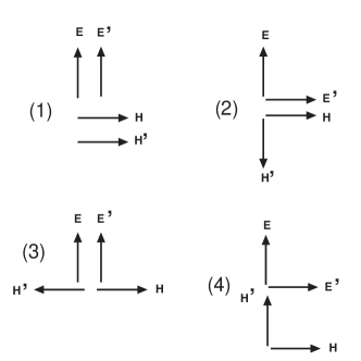
Figure 2: Compton scattering viewed as simultaneous interaction of two electric field vectors ${\bf E},{\bf E^{\prime}}$ and magnetic field vectors ${\bf H},{\bf H^{\prime}}$ for four different cases. (1) Helicity independent forward Compton scattering as given by the amplitude $f_{0}(\omega)$. (2) Helicity dependent forward Compton scattering as given by the amplitude $g_{0}(\omega)$. (3) Helicity independent backward Compton scattering as given by the amplitude $f_{\pi}(\omega)$. (4) Helicity dependent backward Compton scattering as given by the amplitude $g_{\pi}(\omega)$. Longitudinal photons can only provide two electric vectors with parallel planes of linear polarization as shown in the upper part of panel (1). In panels (2) and (4) the direction of rotation leading from ${\bf E}$ to ${\bf E}^{\prime}$ depends on the helicity difference $|\lambda_{p}-\lambda_{\gamma}|$.

Compton scattering in the forward and backward directions lead to more general combinations of electric and magnetic fields. This is depicted in Figure 2. Panel (1) corresponds to the amplitude $f_{0}(\omega)$, i.e. to Compton scattering in the forward direction with parallel electric and magnetic fields. This case can be compared with Eq. (42). Electromagnetic scattering of neutrons corresponds to the upper part of panel (1) where two electric vectors are shown. The cases described in panels (2) – (4) can be realized with real photons only. Panel (2) corresponds to helicity dependent Compton scattering in the forward direction as described by the amplitude $g_{0}(\omega)$. Panel (3) corresponds to the amplitude $f_{\pi}(\omega)$ and panel (4) to the amplitude $g_{\pi}(\omega)$. According to the definitions given in Eq. (41), panel (3) corresponds to the case where a $\sigma$ meson while attached to a constituent quark interacts with the two photons and panel (4) to the case where a $\pi^{0}$ meson while attached to a constituent quark interacts with the two photons.

We have argued that electromagnetic scattering of neutrons corresponds to the upper part of panel (1). Furthermore, we have argued that the reaction $\gamma\gamma\to\sigma\to N\bar{N}$ makes a contribution to the case of panel (3). At a first sight there may be a contradiction to the observation that electromagnetic scattering of neutrons and Compton scattering measure the same electric polarizability. The explanation that there is no contradiction is as follows. In terms of electric and magnetic fields the $\sigma$ meson always makes a contribution if the two field vectors are either parallel or antiparallel. However, with $\alpha(\sigma)=-\beta(\sigma)$ these two parts cancel in the case of panel (1) for real photons but do not cancel for virtual photons at low neutron velocities where magnetic fields are absent.

5.2 Composition of the Compton scattering amplitudes

The total Compton differential cross section is represented via the graphs of Figure 3.

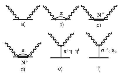
Figure 3: Graphs of processes contributing to Compton scattering by the nucleon³. a) Born terms, b) Compton scattering via nonresonant $1\pi$ excitation of the nucleon, c) Compton scattering via excitation of the resonant states of the nucleon, d) summary of other nonresonant or partly resonant excitation processes of the nucleon contributing to Compton scattering. The corresponding crossed graphs have been omitted. e) pseudoscalar $t$-channel exchange, f) scalar $t$-channel exchange. Regge pole exchanges contributing in the forward direction are not explicitly shown.

Compton scattering takes place via Born terms a) without internal excitation of the nucleon and non-Born terms b) to f) which make contributions to the polarizabilities. The graphs corresponding to the $s$-channel, viz. a) to d), have to be supplemented by crossed graphs which are not shown here. Graph f) is of special interest because it represents the scalar $t$-channel contribution. In addition to the contribution of the $\sigma$ meson there are small contributions of the $f_{0}(980)$ and $a_{0}(980)$ mesons.

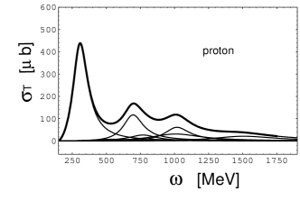
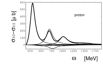
Figure 4: Resonant part of the total photo absorption cross section for $\sigma_{T}=\frac{1}{2}(\sigma_{1/2}+\sigma_{3/2})$ and $\sigma_{3/2}-\sigma_{1/2}$. Thick line: Sum of all resonances. Thin lines: Contributing single resonances.

Figure 4 gives an overview over the spin-independent (left panel) and spin-dependent (right panel) contributions to graph c) of Figure 3. The cross sections are dominated by the $P_{33}(1232)$, $D_{13}(1520)$ and $F_{15}(1680)$ resonances. The main difference between the spin-independent cross section (left panel) and the spin-dependent cross section (right panel) is the enhancement of the $P_{33}(1232)$ contribution by a factor 1.26 which can be traced back to the E2/M1 ratio of the $P_{33}(1232)$ resonance [20]. Without the multipolarity mixing the two resonance curves would be the same for the $P_{33}(1232)$ resonance.

Table 2: Predicted polarizabilities for the proton compared with experimental data. The unit is 10^-4fm³ (for details see [20])

	$\alpha_{p}$	$\beta_{p}$
$P_{33}(1232)$	$-1.1$	+8.3
other resonances	+1.1	+0.2
$E_{0+}$ nonresonant	+3.2	$-0.3$
other nonresonant	+1.3	+1.2
$\sigma$ $t$-channel	+7.6	$-7.6$
$f_{0}$, $a_{0}$ $t$-channel	$-0.1$	+0.1
sum	+12.0	+1.9
experiment	$+12.0\pm 0.6$	$+1.9\mp 0.6$

The nonresonant cross section corresponding to graph b) in Figure 3 has contributions from the single-pion $E_{0+}$, $(M,E)^{(1/2)}_{1+}$ and $M^{(3/2)}_{1-}$ CGLN amplitudes with the $E_{0+}$ contribution being the largest. The polarizabilities of the nucleon have been measured with high precision and compared with predictions from dispersion theory in several investigations. The most recent one is published in [20]. Therefore, it is not necessary to give an extensive coverage of the polarizabilities here but it is sufficient to present the essential results. The $s$-channel contributions $\alpha^{s}$ and $\beta^{s}$ of the electromagnetic polarizabilities have been calculated from the multipole content of the photoabsorption cross section whereas the $t$-channel contribution is given by the transition matrix element ${\cal M}(\sigma\to\gamma\gamma)$ of Eq. (12), the $\sigma$-nucleon coupling constant $g_{\pi NN}=g_{\sigma NN}=13.169\pm 0.057$ [37] and the $\sigma$-meson mass $m_{\sigma}=666$ MeV via $\alpha^{t}=-\beta^{t}={\cal M}(\sigma\to\gamma\gamma)\,g_{\sigma NN}/4\pi m^{2}_{\sigma}=7.6$. Predictions for partial contributions to the polarizabilities of the proton are given in Table 2. The purpose of Table 2 is to show that the experimental data are well understood in terms of excitation processes of the nucleon and that the $\sigma$-meson $t$-channel makes a dominant contribution.

From Table 2 the following conclusions may be drawn: (i) the prediction obtained for the two-photon width $\Gamma(\sigma\to\gamma\gamma)$ from the QLL$\sigma$M has been confirmed with a high level of precision through the excellent agreement of the experimental electric polarizability $\alpha_{p}$ of the proton with the corresponding predicted quantity. (ii) an error for the prediction of $\Gamma(\sigma\to\gamma\gamma)$ may be obtained from the experimental error of $\alpha_{p}$ being $\Delta\alpha_{p}/\alpha_{p}\approx 5\%$. Since the $\sigma$ meson contribution to the electric polarizability is by far the largest it is possible to relate the errors of $\alpha_{p}$ and $\Gamma(\sigma\to\gamma\gamma)$ to each other. Using $\Delta\Gamma(\sigma\to\gamma\gamma)/\Gamma(\sigma\to\gamma\gamma)\approx 2\Delta\alpha_{p}/\alpha_{p}\approx 10\%$ the error given in Eq. (16) is obtained.

6 Observation of the $\sigma$-meson contribution to the differential cross section for Compton scattering

The BEFT sum rule [36] may be derived from the non-Born (nB) part of the invariant amplitude

$${\tilde{A}}_{1}(s,u,t)\equiv A_{1}(s,u,t)-\frac{t}{4\,m^{2}}A_{5}(s,u,t)$$ (43)

by applying the fixed-$\theta$ dispersion relation for $\theta=\pi$

$${\rm Re}{\tilde{A}}^{\rm nB}_{1}=\frac{1}{\pi}{\cal P}\int^{\infty}_{s_{0}}\left(\frac{1}{s^{\prime}-s}+\frac{1}{s^{\prime}-u}-\frac{1}{s^{\prime}}\right){\rm Im}_{s}{\tilde{A}}_{1}(s^{\prime},u^{\prime},t^{\prime})\,ds^{\prime}$$

$$\quad\quad\quad\quad+\frac{1}{\pi}{\cal P}\int^{\infty}_{t_{0}}\,{\rm Im}_{t}{\tilde{A}}_{1}(s^{\prime},u^{\prime},t^{\prime})\frac{dt^{\prime}}{t^{\prime}-t}$$ (44)

with $su=m^{4}$. Then the difference of the electromagnetic polarizabilities is given by

$$\alpha-\beta=-\frac{1}{2\pi}{\rm Re}{\tilde{A}}^{\rm nB}_{1}(s=m^{2},u=m^{2},t=0)=(\alpha-\beta)^{s}+(\alpha-\beta)^{t}.$$ (45)

A calculation analogous to the derivation of the BEFT sum rule (see e.g. [21]) but for general $s$ and $t$ and for the pole representation of the $t$-channel part leads to a generalized BEFT sum rule in the form

$$(\alpha-\beta)^{s}(\omega)=\frac{1}{2\pi^{2}}{\cal P}\int^{\infty}_{\omega_{0}}\sqrt{1+2\frac{\omega^{\prime}}{m}}\,\,\,\frac{\omega^{\prime 3}+\omega^{\prime 2}(m/2)}{\omega^{\prime 3}+\omega^{\prime 2}a(\omega)+\omega^{\prime}b(\omega)+c(\omega)}\,\,\sigma_{f_{\pi}}(\omega^{\prime})\,\,\frac{d\omega^{\prime}}{\omega^{\prime 2}}$$ (46)

$$(\alpha-\beta)^{t}(\omega)=-\frac{1}{2\pi}\,\,\frac{{\cal M}(\sigma\to\gamma\gamma)\,g_{\sigma NN}}{t(\omega)-m^{2}_{\sigma}}$$ (47)

with $\sigma_{f_{\pi}}(\omega)=\sigma(\omega,E1,\,\,M2,\cdots)-\sigma(\omega,M1,\,\,E2,\cdots)$ and

$$a(\omega)=\frac{-4\omega^{2}+2m\omega+m^{2}}{2(m+2\omega)},\,\,\,b(\omega)=-\frac{2m\omega^{2}}{m+2\omega},\,\,\,c(\omega)=-\frac{m^{2}\omega^{2}}{2(m+2\omega)},\,\,\,t(\omega)=-4\frac{\omega^{2}}{1+2\frac{\omega}{m}}.$$ (48)

It should be noted that Eq. (47) follows from the reaction $\gamma\gamma\to\sigma\to N\bar{N}$ where $\sigma$ is a genuine $q\bar{q}$ state. This means that the $\sigma$ meson has a definite mass of $m_{\sigma}=666$ MeV as predicted by the QLL$\sigma$M. A complex mass parameter or a mass distribution are excluded as explained in the text following Eq. (27).

The generalized polarizabilities as defined in (46) and (47) are depicted in Figure 5. The solid curve starting at $(\alpha-\beta)(0)=-9.4$ represents the contribution of the $P_{33}(1232)$ resonance. The solid curve starting at $(\alpha-\beta)(0)=+3.5$ represents the contribution of the nonresonant $E_{0+}$ amplitude. The curves starting at $(\alpha-\beta)(0)=+15.2$ represent the $t$-channel contribution of the $\sigma$-meson calculated for different $\sigma$-meson masses. The upper curve (dark grey or red) has been calculated for $m_{\sigma}=800$ MeV, the middle curve (grey or green) for $m_{\sigma}=600$ MeV and the lower curve (light grey of blue) for $m_{\sigma}=400$ MeV. In principle also a contribution of the $D_{13}(1520)$ resonance has to be taken unto account. This contribution is not shown in order not to overload the figure. The effect of this contribution is to cancel the $E_{0+}$ contribution in the energy range from 400 to 700 MeV which is the most relevant part of the spectrum for the comparison with

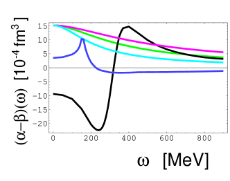
Figure 5: Difference of generalized polarizabilities $(\alpha-\beta)(\omega)$ versus photon energy $\omega$. Solid curve starting at $(\alpha-\beta)(0)=-9.4$: contribution of the $P_{33}(1232)$ resonance. Solid curve starting at $(\alpha-\beta)(0)=+3.5$: Contribution of the nonresonant $E_{0+}$ amplitude. Curves starting at $(\alpha-\beta)(0)=+15.2$: $t$-channel contribution of the $\sigma$-meson calculated for different $\sigma$-meson masses. Upper curve (dark grey or red): $m_{\sigma}=800$ MeV. Middle curve (grey or green): $m_{\sigma}=600$ MeV. Lower curve (light grey or blue): $m_{\sigma}=400$ MeV. Not shown is the contribution of the $D_{13}(1520)$ resonance which cancels the $E_{0+}$ contribution in the relevant energy range from 400 to 700 MeV.

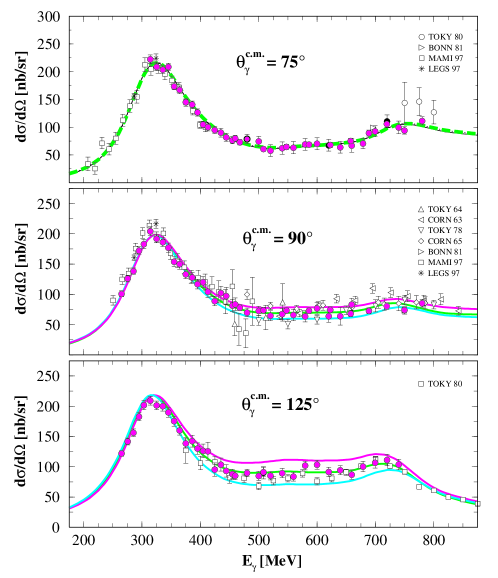
Figure 6: Differential cross sections for Compton scattering by the proton versus photon energy. The three panels contain data corresponding to the c.m.-angles of $75^{0}$, $90^{0}$ and $125^{0}$. The three curves are calculated for different mass parameters $m_{\sigma}=800$ MeV (upper, dark grey or red), 600 MeV (center, grey or green) and 400 MeV (lower, light grey or blue).

experimental data as discussed later. It is apparent that the contribution of the $\sigma$ meson enters via a constructive interference with the contribution of the $P_{33}(1232)$ resonance. This strongly enhances the effects of the $\sigma$ meson in the total differential cross section for Compton scattering at large scattering angles in the range between 400 and 700 MeV.

Differential cross sections for Compton scattering by the proton have been measured at the high duty-factor electron facility MAMI (Mainz) [40, 41]. In this experiment it was possible to cover the total energy range from 250 MeV to 800 MeV and angular range in the laboratory from $30^{\circ}$ to $150^{\circ}$ in one experimental run. The result of this experiment is shown in Figure 6. The experimental data collected in angular intervals are given for the c.m. scattering angles $75^{\circ}$, $90^{\circ}$ and $125^{\circ}$ and compared with predictions based on dispersion theory. As in Figure 5 the mass of the $\sigma$ meson has been varied using 800 MeV, 600 MeV and 400 MeV while keeping the quantity $(\alpha-\beta)(0)$ constant. From kinematical reasons effects of the $\sigma$ meson in the differential cross section for Compton are only expected in the backward direction and are largest at $\theta=180^{\circ}$. This is in agreement with the observations made in Figure 6. At $\theta^{\rm c.m.}=125^{\circ}$ there are three different curves visible in the energy range between 400 MeV and 700 MeV corresponding to the different $\sigma$ masses: 800 MeV (upper), 600 MeV (center) and 400 MeV (lower). This apparently is in a complete agreement with our expectation from Figure 5. This means that we have seen the contribution from the $\sigma$ meson pole in the experimental differential cross section. Furthermore, the mass we have determined is $m_{\sigma}\approx 600$ MeV in agreement with the prediction made by the QLL$\sigma$M for the reaction $\gamma\gamma\to\sigma\to N\bar{N}$, viz. $m_{\sigma}=666$ MeV. This mass corresponds to the location of the pole in the $t$-channel of Compton scattering as outlined above.

7 Discussion

In the present paper we have shown that the evaluation of the reaction $\gamma\gamma\to\sigma\to N{\bar{N}}$ with properties of the $\sigma$ meson as given by the QLL$\sigma$M leads to predictions for the electromagnetic polarizabilities of the nucleon being valid with a high level of precision. This strongly confirms the supposition that the $\sigma$ meson indeed enters into the polarizabilities via the $\gamma\gamma\to\sigma\to N{\bar{N}}$ process with the $\sigma$ meson having a mass of $m_{\sigma}=666$ MeV. An even more direct observation of the $\gamma\gamma\to\sigma\to N{\bar{N}}$ reaction has also been made through its large contribution to the differential cross section for Compton scattering by the proton in the energy range from $\omega=400$ MeV to 700 MeV where such a large contribution is expected. On the quark level this process may be understood as Compton scattering by the $\sigma$ meson while being a part of the constituent quark.

Prior to the discovery [29, 8] of the $\sigma$ meson pole representation of the scalar-isoscalar $t$-channel of Compton scattering with the $\sigma$-meson having a mass of $m_{\sigma}=666$ MeV, it was only possible to construct this quantity from a combination of the two reactions $\gamma\gamma\to\pi\pi$ and $\pi\pi\to N{\bar{N}}$ with the $\sigma$ meson being described via a pole on the second Riemann sheet at $\sqrt{s_{\sigma}}=(441-i\,272)$ MeV. Both procedures are correct and equivalent to each other. But certainly the calculation on the basis of Eq. (28) is easier to perform than the calculation on the basis of Eq. (29). A further result of the present investigation is that rather firm arguments are obtained for the two-photon width of the $\sigma$-meson being $\Gamma(\sigma\to\gamma\gamma)=(2.6\pm 0.3)$ keV, thus removing a large systematic uncertainty left over by different recent evaluations [13, 38, 32, 33, 34, 35] of the $\sigma$-meson pole at $\sqrt{s_{\sigma}}=(441-i\,272)$ MeV.

The $\sigma$ meson was originally introduced by Schwinger [1] in his general attempt to explain symmetry breaking including also the electro-weak (EW) sector. Later on it was shown by Gell-Mann–Levy [2] that the $\sigma$ meson may be used to explain the mass of the nucleon, whereas Higgs later on discussed the EW symmetry breaking in a form which nowadays is generally accepted [42] and which enters into the standard model (SM). Similarities between the $\sigma$ meson and the Higgs boson possibly may go beyond this interchange of names. Since the $\sigma$ meson is well understood on a quark level there have been attempts to use it as a guide for models of the Higgs boson (see e.g. [43, 44] and references therein). At present [45] the SM Higgs boson is excluded at 95% C.L. for a mass lower than 114.4 GeV and for a mass in the range $160<m_{H}<170$ GeV. This result is only valid for the SM Higgs boson and does not contain information about a non-SM Higgs boson [45].

It is interesting to note that in a new development of ChPT the possible role of the $f_{0}(600)$ meson has been discussed [46].

References

- [1] J. Schwinger, Ann Phys. 2, 407 (1957)
- [2] M. Gell-Mann, M. Levy, Nuovo Cimento 16, 705 (1960)
- [3] N.A. Törnqvist, arXiv:hep-ph/0204215.
- [4] F.E. Close, N.A. Törnqvist, J. Phys. G 28, R 249 (2002), arXiv:hep-ph/0204205
- [5] N.A. Törnqvist, Phys. Lett. B 619, 145 (2005), arXiv:hep-ph/0504204
- [6] M.R. Pennington, Int. J. Mod. Phys. A 21, 747 (2006), arXiv:hep-ph/0509265
- [7] R. Delbourgo, M.D. Scadron, Mod. Phys. Lett. A 10, 251 (1995), arXiv:hep-ph/9910242; Int. J. Mod. Phys. A 13, 657 (1998), arXiv:hep-ph/9807504
- [8] M. Schumacher, Eur. Phys. J. A 30, 413 (2006), Eur. Phys. J. A 32, 121 (2007) (E), arXiv:hep-ph/0609040; M.I. Levchuk, A.I. L’vov, A.I. Milstein, M. Schumacher, Proceedings of the Workshop on the Physics of Excited Nucleons, NSTAR2005, 389 (2005), arXiv:hep-ph/0511193
- [9] E. van Beveren, F. Kleefeld, G. Rupp, M.D. Scadron, Phys. Rev. D 79, 098501 (2009), arXiv:0811.2589 [hep-ph]
- [10] I. Caprini, G. Colangelo, H. Leutwyler, Phys. Rev. Lett. 96, 132001 (2006), arXiv:hep-ph/0512364
- [11] E. van Beveren, D.V. Bugg, F. Kleefeld, G. Rupp, Phys. Lett. B 641, 265 (2006), arXiv:hep-ph/0606022
- [12] Particle Data Group, C. Amsler, Phys. Lett. B 667, 1 (2008)
- [13] M.R. Pennington, Phys. Rev. Lett. 97, 011601 (2006), arXiv:hep-ph/0604212
- [14] M.R. Pennington, Mod. Phys. Lett. A22 (2007) 1439, arXiv:0705.3314 [hep-ph]
- [15] E. Klempt, A. Zaitsev, Phys. Rept. 454, 1 (2007), arXiv:0708.4016 [hep-ph]
- [16] M.R. Pennington, in: 11th International Conference on Meson-Nucleon Physics and the Structure of the Nucleon (MENU 2007), Julich, Germany 10-14 Sept. 2007, pp 106, arXiv:0711.1435 [hep-ph]
- [17] M. Schumacher, Eur. Phys. J. A 31, 327 (2007), arXiv:0704.0200 [hep-ph]
- [18] M. Schumacher, Eur. Phys. J. A 34, 293 (2007), arXiv:0712.1417 [hep-ph]
- [19] M. Schumacher, AIP Conference Proceedings 1030 (Workshop on Scalar Mesons and Related Topics Honoring Michael Scadrons’s 70th Birthday - SCADRON70), 129 (2008), arXiv:0803.1074 [hep-ph]; arXiv:0805.2823 [hep-ph]
- [20] M. Schumacher, Nucl. Phys. A 826, 131 (2009), arXiv:0905.4363 [hep-ph]
- [21] M. Schumacher, Progress in Particle and Nuclear Physics 55, 567 (2005), arXiv:hep-ph/0501167
- [22] D. Lurié, A.J. MacFarlane, Phys. Rev. B 136, 816 (1964)
- [23] T. Eguchi, Phys. Rev. D 14, 2755 (1976); 17, 611 (1978)
- [24] U. Vogl, W. Weise, Prog. Part. Nucl. Phys. 27, 195 (1991)
- [25] S.P. Klevansky, Rev. Mod. Phys. 64, 649 (1992)
- [26] V. de Alfaro, S. Fubini, G. Furlan, C. Rossetti, in Currents in Hadron Physics (North Holland, Amsterdam, 1973) Chapt. 5
- [27] T. Hatsuda, T. Kunihiro, Phys. Rep. 247, 221 (1994)
- [28] A.W. Thomas, W. Weise, The Structure of the Nucleon (WILEY-VCJ Berlin, 2000)
- [29] A.I. L’vov, V.A. Petrun’kin, M. Schumacher, Phys. Rev. C 55, 359 (1997)
- [30] A.I. L’vov, A.M. Nathan, Phys. Rev. C 59, 1064 (1999)
- [31] M. Nagy, M.D. Scadron, G.E. Hite, Acta Physica Slovaca 54, 427 (2004), arXiv:hep-ph/0406009
- [32] J. A. Oller, L. Roca, C. Schat, Phys. Lett. B 659, 201 (2008), arXiv:0708.1659 [hep-ph]
- [33] J.A. Oller, L. Roca, Eur. Phys. J. A 37, 15 (2008), arXiv:0804.0309 [hep-ph]
- [34] G. Mennessier, S. Narison, W. Ochs, Phys. Lett. B 665, 205 (2008), arXiv:0804.4452 [hep-ph]; Nucl. Phys. Proc. Suppl. 181-182, 238 (2008), arXiv:0806.4092 [hep-ph]
- [35] M.R. Pennington, T. Mori, S. Uehara, Y. Watanabe, Eur. Phys. J. C 56, 1 (2008), arXiv:0803.3389 [hep-ph]
- [36] J. Bernabeu, T.E.O. Ericson, C. Ferro Fontan, Phys. Lett. 49 B, 381 (1974); J. Bernabeu, B. Tarrach, Phys. Lett. 69 B, 484 (1977)
- [37] S.A. Coon, M.D. Scadron, Phys. Rev. C 23, 1150 (1981); D.V. Bugg, M.D. Scadron, arXiv:hep-ph/0312346; D.V. Bugg, Eur. Phys. J. C 33, 505 (2004)
- [38] J. Bernabeu, J. Prades, Phys. Rev. Lett. 100, 241804 (2008), arXiv:0802.1830 [hep-ph]; J. Prades, J. Bernabeu, in: 14th High-Energy Physics International Conference in Quantum Chromodynamics, Montpellier, France, 1-12 July 2008 (2008), arXiv:0809.2475 [hep-ph]
- [39] D. Babusci, G. Giordano, A.I. L’vov, G. Matone, A.M. Nathan, Phys. Rev. C 58, 1013 (1998)
- [40] G. Galler et al., Phys. Lett. B 501, 245 (2001)
- [41] S. Wolf et al., Eur. Phys. J. A 12, 231 (2001)
- [42] P.W. Higgs, Phys. Letters 12, 132 (1964); Phys. Rev. Lett. 13, 508 (1964); Phys. Rev. 145, 1156 (1966)
- [43] M.D. Scadron, R. Delbourgo, G. Rupp, J. Phys. G 32, 735 (2006), arXiv:hep-ph/0603196
- [44] G.L. Castro, J. Pestieau, Mod. Phys. Lett. A 10, 1155 (1996), arXiv:hep-ph/9504350; Z.Y. Fang, G.L. Castro, J.L. Lucio M., J. Pestieau, Mod. Phys. Lett. A 12, 1531 (1997), arXiv:hep-ph/9612430
- [45] K. Peters, Proceedings of the XXIX PHYSICS IN COLLISION, arXiv:0911.1469 [hep-ex], and private communication
- [46] V. Lensky, V. Pascalutsa, Eur. Phys. J. C DOI 10.1140/epjc/s10052-009-1183-z, arXiv:0907.0451 [hep-ph]