Bloch-Wannier theory of persistent current in a ring made of the band insulator: Exact result for one-dimensional lattice and estimates for realistic lattices

Abstract

It is known that a mesoscopic normal-metal ring pierced by magnetic flux supports persistent current. It was proposed recently that the persistent current exists also in a ring made of a band insulator, where it is carried by electrons in the fully occupied valence band. In this work, persistent currents in rings made of band insulators are analyzed theoretically. We first formulate a recipe which determines the Bloch states of a one-dimensional (1D) ring from the Bloch states of an infinite 1D crystal created by the periodic repetition of the ring. Using the recipe, we derive an expression for the persistent current in a 1D ring made of an insulator with an arbitrary valence band $\epsilon(k)$. To find an exact result for a specific insulator, we consider a 1D ring represented by a periodic lattice of $N$ identical sites with a single value of the on-site energy. If the Bloch states in the ring are expanded over a complete set of $N$ on-site Wannier functions, the discrete on-site energy splits into the energy band. At full filling, the band emulates the valence band of the band insulator and the ring is insulating. It carries a persistent current equal to the product of $N$ and the derivative of the on-site energy with respect to the magnetic flux. This current is not zero if one takes into account that the on-site Wannier function and consequently the on-site energy of each ring site depend on magnetic flux. To derive the current analytically, we expand all $N$ Wannier functions of the ring over the infinite basis of Wannier functions of the constituting infinite 1D crystal and eventually determine the crystal Wannier functions by a method of localized atomic orbitals. In terms of the crystal Wannier functions, the current at full filling arises because the electron in the ring with $N$ lattice sites is allowed to make a single hop from site $i$ to its periodic replicas $i\pm N$. In terms of the ring Wannier functions, the same current is due to the flux dependence of the Wannier functions basis, and the longest allowed hop is from $i$ to $i\pm{\rm Int}(N/2)$ only. Finally, we estimate the persistent current at full filling in a few realistic systems. In particular, the rings made of real band insulators (GaAs, Ge, InAs) with a fully filled valence band and empty conduction band are studied. The current decays with the ring length exponentially due to the exponential decay of the Wannier functions. In spite of that, it can be of measurable size.

I I. Introduction

It is known that a conducting ring pierced by a constant magnetic flux can support persistent electron current circulating around the ring Imry-book . The persistent current is well known to exist in a superconducting ring, and also in a normal-metal ring as long as it is mesoscopic (of size comparable or smaller than the electron coherence length). Early work dealing with persistent current and flux quantization in superconducting rings Byers also contains results relevant to the normal metal rings. Later it was mentioned Bloch that one can have circulating currents for free electrons in ballistic normal-metal rings, and the reference Buttiker proposed that persistent currents should exist in the disordered normal-metal rings. The persistent currents were indeed observed in the disordered normal-metal rings Levy ; Chandrasekhar ; Jariwala ; Bluhm ; Bleszynski as well as in ballistic conducting rings Mailly ; Rabaud . Details are reviewed in various papers Eckern ; Saminadayar ; Feilhauer2 .

One of us recently proposed Mosko that persistent current exists also in a ring made of a band insulator, where it is carried exclusively by Bloch electrons in the fully occupied valence band. The effect is interesting for two reasons Mosko . First, it seems to be the only effect manifesting electron transport in a fully occupied valence band. In a standard conductance measurement, the band insulator is biased by two metallic electrodes and one observes the tunneling of conduction electrons from metal to metal through the energy gap of the insulator. One does not observe the transport of valence band electrons in the insulator. Second, in the fully occupied valence band, Bloch electrons cannot be scattered by phonons or other electrons. Therefore, the electron coherence length should be huge even at room temperature if the valence band is separated from the conduction band by a large energy gap. The persistent current in the insulating ring should thus be observable up to high temperatures as a temperature-independent effect as long as excitations into the (empty) conduction band are negligible. By contrast, persistent currents in metallic rings are observable only at low temperatures. Bleszynski .

We report on a study of persistent currents in rings made of band insulators using the formalism of the Bloch and Wannier functions. It was partly motivated by a pioneering analysis Cheung of persistent currents in a 1D ring-shaped periodic lattice composed of the lattice sites with a single value of the on-site energy. The authors derived persistent current $I$ for spinless electrons at zero temperature assuming that they move along the lattice by means of the nearest-neighbor-site hopping. The result reads

$$I=-\frac{4\pi\Gamma_{1}}{N\phi_{0}}\frac{\sin{\frac{\pi}{N}N_{e}}}{\sin{\frac{\pi}{N}}}\sin{\left[\frac{2\pi}{N}\frac{\phi}{\phi_{0}}\right]},\quad-\frac{\phi_{0}}{2}\leq\phi<\frac{\phi_{0}}{2}\ ,$$ (1)

for odd $N_{e}$ and

$$I=-\frac{4\pi\Gamma_{1}}{N\phi_{0}}\frac{\sin{\frac{\pi}{N}N_{e}}}{\sin{\frac{\pi}{N}}}\sin{\left[\frac{\pi}{N}\left(\frac{2\phi}{\phi_{0}}-1\right)\right]},\quad 0\leq\phi<\phi_{0}\ ,$$ (2)

for even $N_{e}$, where $N_{e}$ is the electron number in the ring, $N$ is the number of the lattice sites, $\phi$ is the magnetic flux piercing the ring, $\phi_{0}\equiv h/e$ is the flux quantum, and $\Gamma_{1}$ is the hopping amplitude. Equations (1) and (2) show a nonzero current for a conductor ($N_{e}<N$). However, they show a zero current for an insulator ($N_{e}=N$), which contradicts our claim that persistent current exists also in an insulating ring.

Therefore, one of our goals is to give exact proof that a ring made of a band insulator does support a non-zero persistent current carried by the fully filled valence band. We also provide a simple tool allowing to estimate persistent currents in rings made of realistic band insulators. We finally present a derivation of an exact persistent current expression for a specific model insulator. This paper is structured as follows.

In Sect. II, we formulate a recipe which determines the Bloch states of a one-dimensional (1D) ring from the Bloch states of an infinite 1D crystal created by the periodic repetition of the ring. In Sect. III we use the recipe to derive an expression for the persistent current in a 1D ring made of a band insulator with an arbitrary valence band $\epsilon(k)$. The expression generally shows that the current is not zero, although it does turn to zero for a cosine-shaped energy band, which was used in the analysis with nearest-neighbor-site hopping Cheung .

To derive an exact result for a specific insulator, in Sect. IV we consider a 1D ring represented by a periodic lattice of $N$ identical sites with a single value of the on-site energy. If the Bloch states in the ring are expanded over a complete set of $N$ on-site Wannier functions, the discrete on-site energy splits into the energy band. At full filling, the band emulates the valence band of the band insulator and the ring is insulating. We find that it carries a persistent current equal to the product of $N$ and the derivative of the on-site energy with respect to the magnetic flux. An alternative explanation of why Eqs. (1) and (2) give zero current at full filling is that they do not take into account the flux-dependence of the on-site energy.

To get closer to an exact formula, in Sect. IV we expand all $N$ Wannier functions of the ring over the basis of Wannier functions of the constituting infinite 1D crystal. In terms of the crystal Wannier functions, the current at full filling arises because the electron in the ring with $N$ lattice sites is allowed to make a single hop from site $i$ to its periodic replicas $i\pm N$. Alternatively, in terms of the ring Wannier functions the same current is due to the flux dependence of the Wannier functions basis, and the longest allowed hop is from $i$ to $i\pm{\rm Int}(N/2)$ only.

In Sect. V we eventually derive the crystal Wannier functions by a method of localized atomic orbitals (LCAO) and express the persistent current at full filling by means of an exact formula. The formula is found to be in good agreement with a numerical LCAO calculation. The numerical data are provided for a 1D ring made of an artificial band insulator, namely for a GaAs ring subjected to a periodic potential emulating the insulating lattice.

In Sect. VI we estimate persistent currents in the rings made of real band insulators (GaAs, Ge, InAs) with a fully filled valence band and empty conduction band. The current at full filling decays with the ring length exponentially due to the exponential decay of the Wannier function tails. In spite of that, it can be of measurable size.

Our results are summarized in Sect. VII. We relate them briefly to the paper by Kohn Kohn1 , which defines the insulating state as a property of the many-body ground state, and which contains a remark implicitly admitting the existence of nonzero persistent current in insulating rings.

We note that some of the results of Sect. V were obtained in the conference contribution Moskova by means of a formally different approach. In another conference paper Nemeth-1 the persistent current at full filling was analyzed for a 1D ring with Kronig-Penney potential.

II II. Elementary theory and the general recipe

To review basic concepts, we consider the circular 1D ring with circumference $L$, pierced by magnetic flux $\phi$. The electrons in such ring are described by the Schrödinger equation

$$\left[\frac{1}{2m}(-i\hbar\frac{d}{dx}+\frac{e\phi}{L})^{2}+V(x)\right]\psi_{\phi}(x)=\varepsilon(\phi)\psi_{\phi}(x),$$ (3)

where $x$ is the electron position along the ring circumference, $m$ is the electron mass, $V(x)$ is an arbitrary potential applied along the ring, $\varepsilon(\phi)$ is the electron eigen-energy, and $\psi_{\phi}(x)$ is the electron wave function. Due to the ring geometry, $\psi_{\phi}(x)$ has to fulfill the periodic condition

$$\psi_{\phi}(x)=\psi_{\phi}(x+L).$$ (4)

We define the wave function $\varphi_{\phi}(x)$ by transformation

$$\varphi_{\phi}(x)=\exp\left(i\frac{2\pi}{L}\frac{\phi}{\phi_{0}}x\right)\psi_{\phi}(x).$$ (5)

Setting $\psi_{\phi}(x)=\exp(-i\frac{2\pi}{L}\frac{\phi}{\phi_{0}}x)\varphi_{\phi}(x)$ into (3) and (4) we obtain the Schrödinger equation

$$\left[-\frac{\hbar^{2}}{2m}\frac{d^{2}}{dx^{2}}+V(x)\right]\varphi_{\phi}(x)=\varepsilon(\phi)\varphi_{\phi}(x)$$ (6)

with the boundary condition

$$\varphi_{\phi}(x+L)=\exp(i2\pi\frac{\phi}{\phi_{0}})\varphi_{\phi}(x).$$ (7)

Here the magnetic flux enters only the boundary condition.

In the ring geometry, $V(x)$ obeys the periodic condition

$$V(x)=V(x+L),$$ (8)

which is the same as for the infinite 1D crystal with lattice constant $L$. Therefore, equation (6) with condition (8) is mathematically identical with the Schrödinger equation

$$\left[-\frac{\hbar^{2}}{2m}\frac{d^{2}}{dx^{2}}+V(x)\right]\varphi_{k}(x)=\varepsilon(k)\varphi_{k}(x),$$ (9)

where $V(x)$ is the infinite periodic potential with period $L$, obtained by the periodic repetition of the ring potential $V(x)$. Equation (9) has the well known Bloch solution

$$\varphi_{k}(x)=\exp(ikx)u_{k}(x),$$ (10)

where the function $u_{k}(x)$ fulfills the periodic condition

$$u_{k}(x)=u_{k}(x+L),$$ (11)

and $k$ is the electron wave vector from the interval $(-\infty,\infty)$. Clearly, the wave function (5) and Bloch solution (10) coincide for $k=\frac{2\pi}{L}\frac{\phi}{\phi_{0}}$. Let us discuss this coincidence in detail.

Consider first the ring with zero magnetic flux. To obtain the wave functions in such ring, it suffices to take the Bloch function (10) and to restrict it by the periodic condition

$$\varphi_{k}(x)=\varphi_{k}(x+L),$$ (12)

which is the condition (7) for $\phi=0$. Due to the condition (12), the wave vector $k$ becomes discrete:

$$k=\frac{2\pi}{L}n,\quad n=0,\pm 1,\pm 2,\ldots\,$$ (13)

Thus, in the ring with zero magnetic flux and specified potential $V(x)$, the eigen-function $\varphi_{n}(x)$ and eigen-energy $\varepsilon_{n}$ can be calculated simply by setting $k=\frac{2\pi}{L}n$ into the Bloch solutions $\varphi_{k}(x)$ a $\varepsilon(k)$, calculated for the same potential $V(x)$ repeated with period $L$ from $x=-\infty$ to $x=\infty$. This recipe can be generalized to nonzero magnetic flux as follows.

Arbitrary magnetic flux $\phi$ can be written in the form

$$\phi=n\phi_{0}+\phi^{,},$$ (14)

where $\phi^{,}$ is the reduced flux from the range $<-\frac{\phi_{0}}{2},\frac{\phi_{0}}{2})$ or alternatively from $<0,\phi_{0})$, and $n$ is one of the values $n=0,\pm 1,\pm 2,\ldots$. Setting (14) into (5) one can write (5) in the form

$$\varphi_{n,\phi^{,}}(x)=\exp\left(i\frac{2\pi}{L}\frac{\phi^{,}}{\phi_{0}}x\right)\psi_{n,\phi^{,}}^{,}(x),$$ (15)

where the function $\psi_{n,\phi^{,}}^{,}(x)\equiv\exp\left(i\frac{2\pi}{L}nx\right)\psi_{\phi}(x)$ obeys the periodic condition $\psi_{n,\phi^{,}}^{,}(x)=\psi_{n,\phi^{,}}^{,}(x+L)$. The boundary condition (7) now reads

$$\varphi_{n,\phi^{,}}^{,}(x+L)=\exp(i2\pi\frac{\phi^{,}}{\phi_{0}})\varphi_{n,\phi^{,}}^{,}(x).$$ (16)

Similarly, in the Bloch function theory it is customary to express the wave vector $k$ by means of the relation

$$k=\frac{2\pi}{L}n+k^{{}^{\prime}},$$ (17)

where $k^{{}^{\prime}}$ is the reduced wave vector from the first Brillouin zone and the integer $n$ plays the role of the energy band number. Using (17) we can write the Bloch function (10) as

$$\varphi_{n,k^{,}}(x)=\exp\left(ik^{,}x\right)u_{n,k^{,}}^{,}(x),$$ (18)

where the function $u_{n,k^{{}^{\prime}}}^{{}^{\prime}}(x)\equiv\exp\left(i\frac{2\pi}{L}nx\right)u_{k}(x)$ fulfills the periodic condition $u_{n,k^{{}^{\prime}}}^{{}^{\prime}}(x)=u_{n,k^{{}^{\prime}}}^{{}^{\prime}}(x+L)$. It is then easy to verify that

$$\varphi_{n,k^{,}}^{,}(x+L)=\exp(ik^{,}L)\varphi_{n,k^{,}}^{,}(x).$$ (19)

The equations (15) and (16) coincide with the equations (18) and (19), respectively, if

$$k^{{}^{\prime}}=\frac{2\pi}{L}\frac{\phi^{,}}{\phi_{0}},$$ (20)

or alternatively, if

$$k=\frac{2\pi}{L}(n+\frac{\phi^{,}}{\phi_{0}}).$$ (21)

One can thus formulate the following general recipe. In the ring with a known potential $V(x)$, the eigen-function $\varphi_{n,\phi^{,}}^{,}(x)\equiv\varphi_{\phi}(x)$ and eigen-energy $\varepsilon_{n}(\phi^{{}^{\prime}})\equiv\varepsilon(\phi)$ can be calculated by setting (20) or (21) into the Bloch solutions $\varphi_{n,k^{,}}(x)\equiv\varphi_{k}(x)$ a $\varepsilon_{n}(k^{,})\equiv\varepsilon(k)$, calculated for the same potential $V(x)$ repeated with period $L$ from $x=-\infty$ to $x=\infty$.

The general recipe holds for any potential $V(x)$ obeying the cyclic condition (8). It therefore holds also for any potential which additionally obeys the periodic condition

$$V(x)=V(x+a),$$ (22)

where $a=L/N$ and $N$ is the (integer) number of periods $a$ within the period $L$. This type of potential will be considered in the rest of the paper. Figure 1 illustrates how an infinite 1D crystal is created from a 1D ring with lattice period $a$ and length $L=Na$. Such crystal is still described by Schrödinger equation (9), except that now $V(x)=V(x+a)$ and consequently $u_{k}(x)=u_{k}(x+a)$. However, the condition $u_{k}(x)=u_{k}(x+L)$ holds as well because $V(x)=V(x+L)$. We can rederive the general recipe briefly, if we compare $u_{k}(x)=u_{k}(x+L)$ with $\psi_{\phi}(x)=\psi_{\phi}(x+L)$ and $\varphi_{k}(x)=\exp(ikx)u_{k}(x)$ with $\varphi_{\phi}(x)=\exp\left(i\frac{2\pi}{L}\frac{\phi}{\phi_{0}}x\right)\psi_{\phi}(x)$. We see that $\varphi_{\phi}(x)$ coincides with $\varphi_{k}(x)$ for $k=\frac{2\pi}{L}\frac{\phi}{\phi_{0}}$.

It remains to express the persistent current. The Bloch electron in state $(n,k^{{}^{\prime}})$ moves with velocity $v_{n}(k^{{}^{\prime}})=\frac{1}{\hbar}\frac{\partial{\varepsilon_{n}(k^{{}^{\prime}})}}{\partial{k^{{}^{\prime}}}}$. We set into the Bloch electron velocity the formula (20). We obtain the expression $v_{n}(\phi^{{}^{\prime}})=\frac{L}{e}\frac{\partial{\varepsilon_{n}(\phi^{{}^{\prime}})}}{\partial{\phi^{{}^{\prime}}}}$, which is the electron velocity in state $(n,\phi^{{}^{\prime}})$ in the ring. The current carried by the electron in state $(n,\phi^{{}^{\prime}})$ reads

$$I_{n}(\phi^{{}^{\prime}})=-\frac{ev_{n}(\phi^{{}^{\prime}})}{L}=-\frac{\partial{\varepsilon_{n}(\phi^{{}^{\prime}})}}{\partial{\phi^{{}^{\prime}}}}.$$ (23)

The total persistent current circulating in the ring is

$$I(\phi^{{}^{\prime}})=-\frac{\partial}{\partial{\phi^{{}^{\prime}}}}\sum_{n}\varepsilon_{n}(\phi^{{}^{\prime}}),$$ (24)

where we sum (at zero temperature) over all occupied states $n=0,\pm 1,\pm 2,\ldots$ up to the Fermi level. In the following text we use the formulas (23) and (24) with symbol $\phi^{{}^{\prime}}$ changed to $\phi$, where $\phi\in<-\frac{\phi_{0}}{2},\frac{\phi_{0}}{2})$ or alternatively $\phi\in<0,\phi_{0})$.

Figure 1: The top figure shows schematically the 1D ring composed of the periodic lattice with $N$ lattice sites ($N=3$), periodicity $a$, and length $L=Na$. For simplicity, the lattice potential of the ring is modeled by a square-well potential $V(x)$. The bottom figure depicts the infinite 1D periodic potential obtained by the periodic repetition of the ring potential.

III III. Persistent current in 1D ring made of a crystal with arbitrary valence band $\varepsilon(k)$

Consider first an infinite 1D crystal created from a 1D ring with the lattice period $a$ and length $L=Na$ as it is illustrated in Fig. 1. Let $\varepsilon_{v}(k)$ be the energy dispersion of the valence band of Bloch electrons in that crystal. The wave vector $k$ in $\varepsilon_{v}(k)$ is supposed to be from the Brillouin zone $<-\frac{\pi}{a},\frac{\pi}{a}>$. In what follows we skip the valence band index ($v$) for simplicity and we use notation $\varepsilon(k)$. We can express $\varepsilon(k)$ by means of the infinite Fourier expansion

$$\varepsilon(k) = a_{0}+a_{1}\cos(ka)+$$

$$a_{2}\cos(2ka)+\dots a_{N}\cos(Nka)+\dots,$$

where

$$a_{0}=\frac{1}{\pi/a}\int_{0}^{\pi/a}\varepsilon(k)dk$$ (26)

and

$$a_{j}=\frac{2}{\pi/a}\int_{0}^{\pi/a}\varepsilon(k)\cos(jka)dk,\quad j=1,2,\dots$$ (27)

Now we apply the general recipe from Sect. II. We set for $k$ in Eq. (LABEL:oneparticleenergyexpansion) the equation $k=\frac{2\pi}{Na}(n+\frac{\phi}{\phi_{0}})$. We obtain the expression for the ring energies $\varepsilon_{n}(\phi)$:

$$\varepsilon_{n}(\phi)\equiv\varepsilon(k_{n}(\phi))=\sum_{j=0}^{\infty}a_{j}\cos\left(k_{n}(\phi)\ ja\right)\ ,$$ (28)

where

$$k_{n}(\phi)\equiv\frac{2\pi}{Na}(n+\frac{\phi}{\phi_{0}})\ .$$ (29)

As shown in appendix A, expansion (28) can also be written in the form

$$\varepsilon_{n}(\phi)=\Omega_{0}+\sum_{j=1}^{M}\Bigl{\{}\Omega^{R}_{j}\cos\left(k_{n}(\phi)\ ja\right)+\Omega^{I}_{j}\sin\left(k_{n}(\phi)\ ja\right)\Bigr{\}}\ ,$$ (30)

where $M={\rm Int}(N/2)$ and the Fourier coefficients $\Omega$ are given by equations (102) and (103). Expressions (28) and (30) are mathematically equivalent, but expression (30) reveals an important difference from the Bloch energy (LABEL:oneparticleenergyexpansion). Generally, the Bloch energy (LABEL:oneparticleenergyexpansion) consists of an infinite number of Fourier terms, with the coefficients $a_{j}$ being independent on magnetic flux $\phi$. On the other hand, expression (30) shows that the Bloch energy in the ring can be expressed through a finite number of Fourier terms, with the Fourier coefficients $\Omega$ depending on $\phi$ [see Eqs. (102) and (103)].

In the rest of this section we use Eq. (28). The same results can be obtained by means of Eq. (30), but derivations are more cumbersome.

Setting Eq. (28) into Eq. (24) we obtain the persistent current

$$I(\phi) = \frac{2\pi}{N}\ \frac{1}{\phi_{0}}\ \sum_{j=1}^{\infty}j\ a_{j}$$ (31)

$$\times \Biggl{[}\cos\left(\frac{2\pi}{N}\frac{\phi}{\phi_{0}}\ j\right)\sum_{n}\sin\left(\frac{2\pi}{N}j\cdot n\right)$$

$$+ \sin\left(\frac{2\pi}{N}\frac{\phi}{\phi_{0}}j\right)\sum_{n}\cos\left(\frac{2\pi}{N}j\cdot n\right)\Biggr{]}\ .$$

If the ring contains $N_{e}$ spinless electrons and $N_{e}$ is odd, summation over $n$ in Eq. (31) includes the occupied states $n=0,\pm 1,\pm 2,\dots,\pm(N_{e}-1)/2$. After simple manipulations

$$I(\phi) = \frac{2\pi}{N}\ \frac{1}{\phi_{0}}\ \sum_{j=1}^{\infty}j\ a_{j}\sin\left(\frac{2\pi}{N}\frac{\phi}{\phi_{0}}\ j\right)$$ (32)

$$\times \left[2\sum_{n=0}^{(N_{e}-1)/2}\cos\left(\frac{2\pi}{N}j\cdot n\right)-1\right]\ .$$

Performing the summation over $n$ we arrive to the formula

$$I(\phi) = \frac{2\pi}{N}\ \frac{1}{\phi_{0}}\Biggl{[}\sum_{\begin{subarray}{c}j=1\\ \qquad j\neq N,2N,\dots\end{subarray}}^{\infty}ja_{j}\sin\left(\frac{2\pi}{N}\frac{\phi}{\phi_{0}}\ j\right)\frac{\sin\left(\frac{\pi}{N}jN_{e}\right)}{\sin\left(\frac{\pi}{N}j\right)}$$ (33)

$$+ N_{e}\sum_{j=N,2N,\dots}^{\infty}ja_{j}\sin\left(\frac{2\pi}{N}\frac{\phi}{\phi_{0}}j\right)\Biggr{]}\ ,$$

where $\phi\in<-\frac{\phi_{0}}{2},\frac{\phi_{0}}{2})$. Note that the first sum in (33) omits the terms $j=N,2N,3N,\dots$, included in the second sum.

If $N_{e}$ is even and $\phi\in<0,\phi_{0})$, we sum in Eq. (31) over the occupied states $n=0,\pm 1,\pm 2,\dots,\pm(N_{e}/2-1),-N_{e}/2$. Similar manipulations as before lead to the result

$$I(\phi) = \frac{2\pi}{N}\ \frac{1}{\phi_{0}}$$ (34)

$$\times \Biggl{[}\sum_{\begin{subarray}{c}j=1\\ \qquad j\neq N,2N,\dots\end{subarray}}^{\infty}ja_{j}\sin\left(\frac{\pi}{N}\left(\frac{2\phi}{\phi_{0}}-1\right)\ j\right)\frac{\sin\left(\frac{\pi}{N}jN_{e}\right)}{\sin\left(\frac{\pi}{N}j\right)}$$

$$+ N_{e}\sum_{j=N,2N,\dots}^{\infty}ja_{j}\sin\left(\frac{2\pi}{N}\left(\frac{\phi}{\phi_{0}}\right)j\right)\Biggr{]}\ ,$$

where $\phi\in<0,\phi_{0})$. The results (33) and (34) hold for the conducting ($N_{e}<N$) as well as insulating ($N_{e}=N$) rings.

For $N_{e}=N$ the first sum on the right hand side of Eqs. (33) and (34) becomes zero and both equations take the form

$$I(\phi)=-(2\pi/\phi_{0})\sum_{j=N,2N,\dots}^{\infty}ja_{j}\sin\left(\frac{2\pi}{N}\frac{\phi}{\phi_{0}}j\right),$$ (35)

where $\phi\in<-\frac{\phi_{0}}{2},\frac{\phi_{0}}{2})$ and $N$ can be even as well as odd. Equation (35) expresses the persistent current in a 1D ring made of a band insulator with an arbitrary valence band $\varepsilon_{k}$.

An important property of the formula (35) can be recognized without specifying the dispersion law $\varepsilon_{k}$. The dispersion $\varepsilon(k)$ is a periodic function of period $2\pi/a$. As long as it is analytic in the whole Brillouin zone $<-\frac{\pi}{a},\frac{\pi}{a}>$, the Fourier coefficients $a_{j}$ in the expansion (LABEL:oneparticleenergyexpansion) obey the inequality Pinsky

$$|a_{j}|\leq Ce^{-\xi j},$$ (36)

where $C$ and $\xi$ are positive constants. Equation (35) combined with inequality (36) shows that the persistent current in the insulating ring is in general not zero albeit it decreases with the ring length at least exponentially. In the next sections, we will demonstrate for various specific insulating rings the exponential decrease, and we will see that the current can be of measurable size in realistic systems.

The pioneer results (1) and (2) can be obtained from Eqs. (33) and (34) if we keep only the term $j=1$ and we put $a_{1}\equiv-2\Gamma_{1}$. Equations (1) and (2) predict for insulating rings ($N_{e}=N$) a zero persistent current, which contradicts equation (35). Origin of this contradiction is evident. Keeping only the term $j=1$ means that only the nearest-neighbor-site hopping is operative. This approach, also known as tight-binding approximation, simplifies the general dispersion law (LABEL:oneparticleenergyexpansion) to the cosine shaped dispersion $\varepsilon(k)\propto\cos(ka)$. However, equation (35) shows that nonzero persistent current in the insulating ring of length $N$ is (mainly) due to the Fourier coefficient $a_{N}$ which is in general not zero for a realistic dispersion law. We will see in the next section that $a_{N}$ physically represents the hopping amplitude for a single hop from site $i$ to its periodic replicas $i\pm N$.

IV IV. Persistent current in insulating 1D ring in the Wannier functions formalism

We consider again the 1D ring with lattice period $a$ and length $L=Na$, sketched in Fig. 1. Simultaneously, we consider the infinite 1D crystal obtained by the periodic repetition of the 1D ring, as it is illustrated in Fig. 1. For the sake of clarity we recall a few major points. First, the Bloch function $\varphi_{k}(x)$ and Bloch energy $\varepsilon(k)$ in the infinite crystal are described by Schrödinger equation

$$H\varphi_{k}(x)=\varepsilon(k)\varphi_{k}(x)\ ,$$

$$H=-\frac{\hbar^{2}}{2m}\frac{d^{2}}{dx^{2}}+V(x),\quad V(x)=V(x+a).$$ (37)

Second, according to the general recipe of Sect. II, the Bloch function and Bloch energy in the ring, $\varphi_{n,\phi}(x)$ and $\varepsilon_{n}(\phi)$, are given by equations

$$\varphi_{n,\phi}(x)=\varphi_{k=k_{n}(\phi)}(x),\quad\varepsilon_{n}(\phi)=\varepsilon(k=k_{n}(\phi))\ ,$$

$$k_{n}(\phi)\equiv\frac{2\pi}{Na}(n+\frac{\phi}{\phi_{0}})\ .$$ (38)

Third, the Bloch vector $k$ is assumed to be from the Brillioun zone $<-\frac{\pi}{a},\frac{\pi}{a}>$, or alternatively from $<0,\frac{2\pi}{a}>$. This means that $\varepsilon(k)$ is the dispersion of a single energy band and $\varphi_{k}(x)$ are the Bloch functions of that band. As before, the functions $\varphi_{k}(x)$ and $\varepsilon(k)$ do not involve any band index, and $\varepsilon(k)$ is supposed to represent the valence band of the crystal. Below we define the Wannier functions by restricting us to the Bloch states of that valence band.

IV.1 A. Wannier functions of the infinite crystal

We first define the Wannier functions for the crystal. According to a standard textbook definition, the Wannier function $W(x-la)$ at the lattice site $x=la$ is defined as

$$W(x-la)\equiv W_{l}(x)=\frac{a}{2\pi}\int_{-\frac{\pi}{a}}^{\frac{\pi}{a}}\ e^{-ikla}\Phi_{k}(x)dk\ ,$$ (39)

where $\Phi_{k}(x)$ is the Bloch function of the infinite crystal. We note that $\Phi_{k}(x)$ is the same Bloch function as $\varphi_{k}(x)$ in equation (37). The only difference is that $\Phi_{k}(x)$ is normalized as

$$\int_{0}^{a}\ \mid\Phi_{k}(x)\mid^{2}\ dx=1\$$ (40)

while the normalization of $\varphi_{k}(x)$ in the infinite crystal is unspecified. In the following text, $\Phi_{k}(x)$ represents the normalized Bloch function of the infinite crystal and the symbol $\varphi_{k}(x)$ with $k=k_{n}(\phi)$ represents the Bloch function of the ring. [In the ring $\varphi_{k}(x)$ is normalized by equation (48).]

Since the crystal is infinite, $k$ is a continuous variable and the Bloch functions fulfill the orthogonality condition

$$\int_{-\infty}^{\infty}\Phi_{k^{\prime}}(x)^{*}\Phi_{k}(x)\ dx=\frac{2\pi}{a}\delta(k^{\prime}-k)\ .$$ (41)

One can then easy verify the orthogonality condition for the Wannier functions,

$$\int_{-\infty}^{\infty}W_{l^{\prime}}^{*}(x)W_{l}(x)\ dx=\delta_{l,l^{\prime}}\ .$$ (42)

Finally, definition (39) can also be written in the inverted form

$$\Phi_{k}(x)=\sum_{l}\ e^{ikla}W_{l}(x)$$ (43)

where one sums over all lattice points of the (infinite) crystal.

We define the matrix elements $\Gamma_{j}$ by equations

$$\Gamma_{l^{\prime},l}=-\int_{-\infty}^{\infty}W_{l^{\prime}}(x)\hat{H}W_{l}(x)dx=\Gamma_{l-l^{\prime}}\ ,\ \ \ \Gamma_{j}\equiv\Gamma_{l-l^{\prime}},$$ (44)

where $l,l^{\prime}=0,\pm 1,\pm 2,\dots\pm\infty$ and it is taken into account that $\Gamma_{l^{\prime},l}$ depends only on the difference $j=l-l^{\prime}$. The Bloch energy $\epsilon(k)$ can be written as $\epsilon(k)=\langle\Phi_{k}|\hat{H}|\Phi_{k}\rangle/\langle\Phi_{k}|\Phi_{k}\rangle$. If we set for $\Phi_{k}$ equation (43), we easy find

$$\varepsilon(k)={\it\Gamma}_{0}+2\sum_{j=1}^{\infty}{\it\Gamma}_{j}\ \cos{jka}.$$ (45)

Comparison of Eq. (45) with Eq. (LABEL:oneparticleenergyexpansion) shows that $a_{j}=2\Gamma_{j}$. Obviously,

$$\Gamma_{j}=\frac{1}{\pi/2a}\int_{-\pi/a}^{\pi/a}\varepsilon(k)\cos(jka)dk,$$ (46)

which is an alternative form of equation (44).

Finally, setting $a_{j}=2\Gamma_{j}$ into the result (35) we get

$$I=-(4\pi/\phi_{0})\sum_{j=N,2N,\dots}^{\infty}j\Gamma_{j}\sin\left(\frac{2\pi}{N}\frac{\phi}{\phi_{0}}j\right)\ .$$ (47)

Equation (47) together with Eq. (44) express the persistent current in the insulating ring through the Wannier functions of the constituting infinite crystal. We defer discussion of these expressions to subsection C, where equation (47) is derived from the Wannier functions of the ring.

IV.2 B. Wannier functions of the ring

Let us define the Wannier functions of the ring. In the ring with $N$ lattice sites and a fixed value of magnetic flux only the discrete Bloch vectors $k_{n}(\phi)$ are allowed, where $k_{n}(0)\in<-\frac{\pi}{a},\frac{\pi}{a}>$ or alternatively $k_{n}(0)\in<0,\frac{2\pi}{a}>$. In both cases there are $N$ allowed values of $n$ (specified below), which means that the originally continuous band $\varepsilon(k)$ consists of $N$ discrete levels $\varepsilon_{n}(\phi)$. The eigen-functions of these levels represent a complete set of $N$ Bloch functions obeying the orthogonality condition

$$\int_{0}^{Na}\ \varphi_{{k}^{\prime}}^{*}(x)\varphi_{k}(x)\ dx=\delta_{{k},{k}^{\prime}}=\delta_{{n},{n}^{\prime}}\ ,$$ (48)

where $k=k_{n}(\phi)$. Consequently, in the 1D ring with $N$ lattice sites the Wannier function at site $x=la$ can be defined as

$$w(x-la)\equiv w_{l}(x)=\frac{1}{\sqrt{N}}\sum_{k}e^{-ikla}\varphi_{k}(x)\ ,$$ (49)

where $k=k_{n}(\phi)$ and summation over $k$ means the summation over the $N$ allowed values of $n$. Definition (49) coincides with definition (3.7) in Kohn’s paper Kohn1 , except that Kohn assumes $k=k_{n}(0)$.

In the following calculations we choose the Brillouin zone $k_{n}(0)\in<0,\frac{2\pi}{a}>$, for which the allowed $n$ are simply

$$n=0,1,\dots,N-1$$ (50)

without regards to the parity of $N$ and sign of $\phi$.

Using Eqs. (48) and (49) we can easy verify the orthogonality condition

$$\int_{0}^{Na}w_{l^{\prime}}(x)^{*}w_{l}(x)\ dx=\delta_{l^{\prime},l}\ .$$ (51)

Finally, definition (49) can also be written in the inverted form

$$\varphi_{k}(x)=\frac{1}{\sqrt{N}}\sum_{l=0}^{N-1}e^{ikla}w_{l}(x)\ .$$ (52)

In this paper the Wannier functions $w_{l}(x)$ are often called the ring Wannier functions while the Wannier functions $W_{l}(x)$ are called the crystal Wannier functions. The ring Wannier functions are magnetic-flux dependent, the crystal Wannier functions are not.

We note that the results obtained in the rest of this section can also be obtained by choosing $k_{n}(0)\in<-\frac{\pi}{a},\frac{\pi}{a}>$. In that case the allowed values of $n$ are

$$n=0,\pm 1,\pm 2,\dots,\pm(N-1)/2$$ (53)

for odd $N$, while for even $N$ one has

$$n=0,\pm 1,\pm 2,\dots,\pm(N/2-1),-N/2\quad\text{for $\phi>0$}$$ (54)

and

$$n=0,\pm 1,\pm 2,\dots,\pm(N/2-1),+N/2\quad\text{for $\phi<0$}.$$ (55)

Evidently, it is more straightforward to work with Eq. (50).

Now we express the persistent current at full filling in terms of the ring Wannier functions. We write $\varepsilon_{n}(\phi)$ in the form

$$\varepsilon_{n}(\phi)=\int_{0}^{Na}\varphi_{k_{n}(\phi)}^{\ast}(x)H\varphi_{k_{n}(\phi)}(x)dx\ .$$ (56)

We need to rewrite the right hand side of Eq. (56) in terms of the matrix elements

$$T_{l^{\prime},l}=\int_{0}^{Na}\ w^{*}_{l^{\prime}}(x)\ H\ w_{l}(x)\ dx\ ,$$ (57)

where $l,l^{\prime}=0,1,\dots N-1$. We set into Eq. (57) the equation (49). We find

$$T_{l^{\prime},l} = \frac{1}{N}\sum_{{n}^{\prime}}\sum_{n}e^{i{k_{n}}^{\prime}(\phi)l^{\prime}a}e^{-i{k_{n}(\phi)}la}$$

$$\times \int_{0}^{Na}\varphi^{*}_{{k_{n}}^{\prime}(\phi)}(x)H\varphi_{k_{n}(\phi)}(x)\ dx$$

$$= \frac{1}{N}e^{i\frac{2\pi}{N}\frac{\phi}{\phi_{0}}(l^{\prime}-l)}\sum_{n=0}^{N-1}e^{i\frac{2\pi}{N}n(l^{\prime}-l)}\varepsilon_{n}(\phi)\ .$$

Since $T_{l^{\prime},l}$ depends only on the difference between $l$ and $l^{\prime}$, we can write

$$T_{l^{\prime},l}=T_{l^{\prime}-l}\equiv T_{j}=\frac{1}{N}e^{i\frac{2\pi}{N}\frac{\phi}{\phi_{0}}j}\sum_{n=0}^{N-1}e^{i\frac{2\pi}{N}nj}\varepsilon_{n}(\phi)\ .$$ (59)

Inverting Eq. (59) we get

$$\varepsilon_{n}(\phi)=\sum_{j=0}^{N-1}\ e^{-ik_{n}(\phi)ja}T_{j}\ .$$ (60)

By means of Eq. (60), the ground state energy of the fully filled valence band is readily obtained in the form

$$E(\phi)=\sum_{n=0}^{N-1}\varepsilon_{n}(\phi)=N\cdot T_{0}(\phi)\ .$$ (61)

Finally, the persistent current at full-filling reads

$$I\ =\ -\frac{dE}{d\phi}\ =\ -N\frac{dT_{0}}{d\phi}\ .$$ (62)

One can see from Eq. (57) that the matrix element $T_{0}$ represents the on-site energy of the Wannier state $w_{l}(x)$. Since $w_{l}(x)$ depends on magnetic flux, so does $T_{0}$. This however means that the current (62) is in general not zero. We have thus arrived at the same conclusion as in the preceding section, where the persistent current in the insulating ring (Eq. 35) was derived from the Bloch states and general recipe.

IV.3 C. Ring Wannier functions in the basis of crystal Wannier functions

The result (47), or equivalently the result (35), can be obtained from the result (62), if the ring Wannier functions are expanded over the basis of the crystal Wannier functions. To show this we proceed as follows.

The Bloch functions of the ring are given by Eq. (38) and normalized as $\int_{0}^{Na}\ \varphi_{k}^{*}(x)\varphi_{k}(x)\ dx=1$, where $k=k_{n}(\phi)$ [see Eq. (48)]. The Bloch functions $\phi_{k}(x)$ coincide with $\varphi_{k}(x)$ except for the normalization constant. As they are normalized by means of Eq. (40), in the ring we have the relation

$$\varphi_{k}(x)=\frac{1}{\sqrt{N}}\phi_{k}(x)\ ,\quad\quad k=k_{n}(\phi)\ ,$$ (63)

We set for $\phi_{k}(x)$ in Eq. (63) the definition (43). Then we set Eq. (63) into the right hand side of Eq. (49). We obtain

$$w_{l}(x)=\frac{1}{N}\sum_{k}\sum_{l^{\prime}=-\infty}^{\infty}e^{-ik(l-l^{\prime})a}W_{l^{\prime}}(x)\ ,$$ (64)

where $k=k_{n}(\phi)$ and summation over $k$ means the summation over $n=0,1,\dots,N-1$. Using substitution $l^{\prime}=Nr+s$, where $s=0,1,\dots(N-1)$ and $r=0,\pm 1,\pm 2,\dots\pm\infty$, we further obtain

$$w_{l}(x) = \sum_{r=-\infty}^{\infty}\sum_{s=0}^{N-1}\ W_{Nr+s}(x)e^{i\frac{2\pi}{N}\frac{\phi}{\phi_{0}}(rN+s-l)}$$

$$\times \frac{1}{N}\sum_{n=0}^{N-1}e^{i\frac{2\pi}{N}n(s-l)}\ .$$

Eventually

$$w_{l}(x)=\sum_{r=-\infty}^{\infty}e^{i2\pi\frac{\phi}{\phi_{0}}r}\ W_{Nr+l}(x)\ .$$ (66)

Equation (66) expresses the ring Wannier function at the ring site $l$, $w_{l}(x)$, through the crystal Wannier functions $W_{l^{\prime}}(x)$. For $\phi=0$ equation (66) coincides with equation (5.9) in Kohn’s paper Kohn1 .

Setting Eq. (66) into Eq. (57) we obtain

$$T_{j}=\int_{0}^{Na}\ w^{*}_{j}(x)\ \hat{H}\ w_{0}(x)\ dx$$

$$= \sum_{r=-\infty}^{\infty}\sum_{r^{\prime}=-\infty}^{\infty}e^{i2\pi\frac{\phi}{\phi_{0}}(r-r^{\prime})}\int_{0}^{Na}W_{Nr^{\prime}+j}(x)\hat{H}W_{Nr}(x)dx$$

$$= \sum_{s=-\infty}^{\infty}e^{-i2\pi\frac{\phi}{\phi_{0}}s}\sum_{r^{=}-\infty}^{\infty}\int_{0-rNa}^{Na-rNa}\ W_{Ns+j}(x)\hat{H}W_{0}(x)dx$$

$$= \sum_{s=-\infty}^{\infty}e^{-i2\pi\frac{\phi}{\phi_{0}}s}\int_{-\infty}^{\infty}\ W_{Ns+j}(x)\hat{H}W_{0}(x)dx\ .$$

By means of the matrix elements $\Gamma_{j}$, equation (LABEL:Tgeneral1) can be written as

$$T_{j}=\sum_{s=-\infty}^{\infty}e^{-2\pi i\frac{\phi}{\phi_{0}}s}\Gamma_{sN+j}\ .$$ (68)

For $j=0$ equation (68) gives

$$T_{0}=\Gamma_{0}+2\sum_{s=1}^{\infty}\ \Gamma_{sN}\cos(2\pi\frac{\phi}{\phi_{0}}s)\ .$$ (69)

We substitute Eq. (69) into the right hand side of Eq. (62). We obtain the persistent current at full filling in the form

$$I=-\frac{4\pi N}{\phi_{0}}\sum_{s=1}^{\infty}\ s\ \Gamma_{sN}\ \sin(2\pi\frac{\phi}{\phi_{0}}s)\ ,$$ (70)

or equivalently in the form (47) which coincides with the result (35) for $a_{j}=2\Gamma_{j}$.

In the rest of this section we discuss the physical meaning of the coefficients $\Gamma_{N}$, $\Gamma_{2N}$, etc., appearing in expression (47). Since $a_{j}=2\Gamma_{j}$, the meaning of the coefficients $a_{N}$, $a_{2N}$, etc., is the same and does not need an extra discussion.

According to the definition (44), in the infinite 1D crystal the matrix element $\Gamma_{N}$ represents the hopping amplitude of a single hop from the Wannier state at site $l$ to the Wannier state at site $l+N$. In the ring with $N$ lattice sites the site $l+N$ is a periodic replica of site $l$, which means the same site. Appearance of $\Gamma_{N}$ in expression (47) therefore implies, that the electron in the ring with $N$ sites can make a single hop from the Wannier state at site $l$ to its periodic replica at site $l+N$. In other words, the electron hops from site $l$ to the same site by making one round around the ring, and $\Gamma_{N}$ is the hopping amplitude of the process. Note that we speak about hopping in the ring, but in terms of the Wannier states of the infinite crystal (c.f. Eq. 44).

Similarly, the coefficient $\Gamma_{2N}$ describes the process in which the electron hops from site $l$ to the same site by making two rounds around the ring. It follows from relation (36) and equation $a_{j}=2\Gamma_{j}$, that $\Gamma_{2N}$ is much smaller than $\Gamma_{N}$. Its contribution to the right hand side of Eq. (47) is therefore negligible. The meaning of the coefficients $\Gamma_{3N}$, $\Gamma_{4N}$, etc., is analogous and their contribution is negligible even more.

We can summarize the result (47) as follows. The persistent current in the insulating ring with $N$ lattice sites, derived in terms of the crystal Wannier functions, is due to the fact that the electron at the ring site $l$ is allowed to make a single hop from site $l$ to its periodic replicas $l\pm N$. (The sign minus is allowed as well due to the symmetry reason.)

The process in which an electron at the ring site $l$ hops from site $l$ to the same site by making one round around the ring may seem meaningless, because such process does not exist in the basis of the ring Wannier functions. In that basis the energy spectrum $\varepsilon_{n}(\phi)$ is given by equation (60). As shown in appendix B, equation (60) can be rewritten for odd $N$ as

$$\varepsilon_{n}(\phi)=\sum_{j=-\frac{N-1}{2}}^{\frac{N-1}{2}}\ e^{-i{k_{n}(\phi)}ja}T_{j}\ ,$$ (71)

and for even $N$ as

$$\varepsilon_{n}(\phi)=\sum_{j=-\frac{N}{2}+1}^{\frac{N}{2}}\ e^{-i{k_{n}(\phi)}ja}T_{j}\ ,$$ (72)

where $T_{-j}=T^{*}_{j}$. According to the definition (57), the matrix element $T_{j}$ represents the amplitude of hopping from the ring Wannier state $w_{l}(x)$ to the ring Wannier state $w_{l^{\prime}}(x)$, with $j=l-l^{\prime}$ being the hopping length. The maximum hopping length between the ring Wannier states, allowed by equations (71) and (72), is $j=\pm{\rm Int}(N/2)$ only, and the current in the insulating ring (Eq. 62) is due to the fact that the ring Wannier states depend on magnetic flux. Hopping from $l$ to $l\pm N$, $l\pm 2N$, etc., emerges after the ring Wannier states are expressed (see Eq. 64) through the flux-independent crystal Wannier states. This provides a different picture of the same physics.

V V. The LCAO approximation, application to the 1D lattice with rectangular potential wells

To evaluate the persistent current (Eq. 47) for a specific crystal lattice, we need to determine the crystal Wannier functions of the lattice. As an example we consider the ring-shaped 1D lattice in Fig. 2. The lattice is composed of the artificial 1D atoms with a single atomic level $\epsilon_{a}$. The atomic orbital $\varphi_{a}(x)$ and energy $\epsilon_{a}$ in the isolated atom positioned at $x=0$ obey the Schrödinger equation

$$\left[-\frac{\hbar^{2}}{2m}\frac{d^{2}}{dx^{2}}+v(x)\right]\varphi_{a}(x)\ =\ \epsilon_{a}\varphi_{a}(x)\ ,$$ (73)

where $v(x)$ is the atomic potential modeled as a rectangular potential well centered at $x=0$ (figure 2, left).

Figure 2: Left: One-dimensional model of a single isolated atom, described by equation (73). The atomic potential, $v(x)$, is modeled by the potential well of width $2d$, embedded between two infinitely-thick potential barriers of height $V_{0}$. Right: The potential $V(x)$ in a ring-shaped periodic lattice composed of $N$ one-dimensional atoms ($N=6$). The lattice period is $a$, the ring circumference is $L=Na$. In the numerical calculations of Sect. V, the parameters of the ring are chosen to emulate the GaAs ring with conduction electrons subjected to the periodic potential of $N$ quantum dots: the electron effective mass is $m=0.067m_{0}$, the period of the quantum-dot lattice is $a=40$nm, the ring length is $L=Na$, and the size and depth of the potential well (quantum dot) are $2d=15$nm and $V_{0}=18$meV, respectively. For these parameters the potential well supports one bound state, the ground state with energy $\varepsilon_{a}=-10.4$meV. The ground-state orbital $\varphi_{a}(x)$ is sketched schematically.

In accord with the general recipe of Sect. II, assume that the ring with $N$ atoms (figure 2, right) is periodically repeated as shown in figure 1. This repetition gives rise to the infinite 1D crystal with potential $V(x)$ which is periodic with period $a$ and ranges from $x=-\infty$ to $x=\infty$. Evidently, $V(x)$ is a sum of all isolated atomic potentials, that means

$$V(x)\ =\ \sum_{l=-\infty}^{\infty}\ v(x-la)\ ,$$ (74)

where $la$ is the position of the $l$-th lattice point. The Bloch function $\Phi_{k}(x)$ and Bloch energy $\epsilon(k)$ of the electron moving in such periodic potential can be expressed analytically in the approximation of localized atomic orbitals (LCAO). The Bloch function is approximated by the LCAO ansatz Ashcroft

$$\Phi_{k}(x)\ =\ C\sum_{l=-\infty}^{\infty}\ e^{ikla}\varphi_{a}(x-la)\ ,$$ (75)

where $\varphi(x-la)$ is the atomic orbital at the lattice point $la$ and $C$ is the normalization constant (given below). The Bloch energy $\epsilon(k)$ can be expressed as

$$\epsilon(k)=\langle\Phi_{k}|\hat{H}|\Phi_{k}\rangle/\langle\Phi_{k}|\Phi_{k}\rangle,$$ (76)

where

$$\hat{H}=-\frac{\hbar^{2}}{2m}\frac{d^{2}}{dx^{2}}+V(x),\ \ \ V(x)\ =\ \sum_{l=-\infty}^{\infty}\ v(x-la)\ .$$ (77)

If we use the LCAO ansatz (75), a simple textbook calculation Ashcroft gives the formula

$$\epsilon(k)=\epsilon_{a}-\frac{\gamma_{0}+2\sum_{j=1}^{\infty}\gamma_{j}\cos{(kja)}}{1+2\sum_{j=1}^{\infty}\alpha_{j}\cos{(kja)}},\$$ (78)

where

$$\alpha_{j}=\int_{-\infty}^{\infty}dx\varphi_{a}(x-ja)\varphi_{a}(x),$$ (79)

$$\gamma_{j}=-\int_{-\infty}^{\infty}dx\varphi_{a}(x-ja){V^{\prime}}(x)\varphi_{a}(x),\quad\gamma_{0}=\gamma_{j=0},$$ (80)

and

$${V^{\prime}}(x)=V(x)-v(x),$$ (81)

with $v(x)$ being the atomic potential at the lattice site $l=0$. In Appendix C we express $\alpha_{j}$ and $\gamma_{j}$ analytically for the model atomic lattice of Fig. 2.

Using the general recipe of section II, we obtain the spectrum of the ring, $\epsilon_{n}(\phi)$, directly from the Bloch energy (78). It reads

$$\epsilon_{n}(\phi)=\epsilon_{a}-\frac{\gamma_{0}+2\sum_{j=1}^{\infty}\gamma_{j}\cos{[k_{n}(\phi)ja]}}{1+2\sum_{j=1}^{\infty}\alpha_{j}\cos{[k_{n}(\phi)ja]}},$$ (82)

where $k_{n}(\phi)\equiv\frac{2\pi}{Na}(n+\frac{\phi}{\phi_{0}})$. One can substitute the spectrum (82) into the persistent current formula (24) and one can evaluate the sum on the right hand side of Eq. (24) numerically. We will refer to this approach as to the numerical LCAO approach. The approach provides a straightforward numerical evaluation of persistent current in insulating rings ($N_{e}=N$) as well as in conducting rings ($N_{e}<N$). It does not provide understanding of the effect, however, it is useful for verification of analytical results.

We mainly want to verify our result for insulating rings, the formula (47). For a meaningful comparison with the numerical LCAO approach, the hopping amplitude $\Gamma_{j}$ in the formula (47) has to be determined in the LCAO approximation.

We start by specifying the constant $C$ in the ansatz (75). Setting Eq. (75) into the normalization condition (40) we find

$$\frac{1}{\mid C\mid^{2}}=1+2\sum_{j=1}^{\infty}\alpha_{j}\cos jka\equiv N(k)\ .$$ (83)

The same result is obtained if we set Eq. (75) into the orthogonality condition (41).

The crystal Wannier functions are defined by equation (39). We set into equation (39) the ansatz (75) with $C=1/\sqrt{N(k)}$. We obtain the crystal Wannier function in the form Kohn2 ; Andreoni

$$W_{l}(x)=\sum_{l^{\prime}=-\infty}^{\infty}\ c_{l^{\prime}-l}\ \varphi_{a}(x-l^{\prime}a)\ ,$$ (84)

where

$$c_{n}=\frac{a}{2\pi}\int_{-\frac{\pi}{a}}^{\frac{\pi}{a}}\frac{\cos{(kna)}}{\sqrt{N(k)}}\ dk\ .$$ (85)

Expression (84) is the crystal Wannier function in the LCAO approximation. It is easy to verify that the expression (84) fulfills the orthogonality condition (41) exactly.

If we express the crystal Wannier functions in Eq. (44) by means of equation (84), we find that

$${\it\Gamma}_{j}=\sum_{n=-\infty}^{\infty}\sum_{n^{\prime}=-\infty}^{\infty}c_{n-j}\ c_{n^{\prime}}\left(\varepsilon_{a}\alpha_{n-n^{\prime}}-\gamma_{n-n^{\prime}}\right)\ .\$$ (86)

Equation (86) is the hopping amplitude $\Gamma_{j}$ in the LCAO approximation. An alternative form of Eq. (86) is the equation

$$\Gamma_{j} = \frac{a}{2\pi}\int_{-\pi/a}^{\pi/a}dk\cos(jka)$$

$$\times \left[\epsilon_{a}-\frac{\gamma_{0}+2\sum_{j^{\prime}=1}^{\infty}\gamma_{j^{\prime}}\cos{(kj^{\prime}a)}}{1+2\sum_{j^{\prime}=1}^{\infty}\alpha_{j^{\prime}}\cos{(kj^{\prime}a)}}\right]\ ,$$

obtained by setting the Bloch energy (78) into the Fourrier transformation (46).

We also note that the Bloch energy (78) is an alternative form of the expression (45) with coefficients $\Gamma_{j}$ given by equation (86), since both forms follow from the same LCAO approximation. Proof of coincidence of both forms is straightforward, but lengthy and therefore not shown.

The LCAO expression (86) together with expressions (85) and (83) are still complicated for analytical calculations. Fortunately, the expressions can be simplified, if we take into account that the coefficients $\alpha_{j}$ and $\gamma_{j}$ decay with increasing $j$ exponentially. Exponential decay is due to the fact that the atomic orbitals $\varphi_{a}$ are exponentially localized at the lattice sites, which is the case for any realistic orbital. If the localization is strong enough, then $1\gg\mid\alpha_{1}\mid\gg\mid\alpha_{2}\mid\gg\dots$ and $1\gg\mid\gamma_{1}\mid\gg\mid\gamma_{2}\mid\gg\dots$. In that limit the expressions (85) and (86) are calculated in appendix D. The results are

$$c_{n}\simeq(-\alpha_{1})^{n}\mid A_{n}\mid\ ,\ \ \ n\geq 0\ ,\ \ \ c_{-n}=c_{n}\ ,$$ (88)

where $A_{0}=1$ and

$$A_{n}=(-1)^{n}\frac{1}{2^{2n}}\ \binom{2n}{n}\simeq(-1)^{n}\frac{1}{\sqrt{\pi n}}\ ,\ \ n\geq 1\ ,$$ (89)

and

$${\it\Gamma}_{j}\simeq-\gamma_{1}(-\alpha_{1})^{(j-1)}\ ,\ \ \ \ j\geq 1.$$ (90)

Expressing $\Gamma_{j}$ in equation (47) by means of Eq. (90) and keeping only the term with $j=N$ we obtain the result

$$I(\phi)=-\ \frac{2\pi}{\phi_{0}}\ \gamma_{1}\ N\ (-\alpha_{1})^{(N-1)}\sin\left(2\pi\frac{\phi}{\phi_{0}}\right)\ .$$ (91)

The last equation is the persistent current in the insulating ring in the LCAO approximation. The following features of the result (91) are worth stressing.

For positive $\alpha_{1}$ equation (91) predicts the exponentially decaying current with alternating sign, $I(N)\sim(-\alpha_{1})^{(N-1)}$. Just this result holds for the ring in figure 2. Indeed, $\alpha_{1}$ is positive for a positive $\varphi_{a}(x)$ such like the ground state orbital in figure 2, which follows from definition (79) as well as from the final expression for $\alpha_{j}$ (appendix C).

For negative $\alpha_{1}$ the dependence $I(N)\sim(-\alpha_{1})^{(N-1)}$ implies the exponentially decaying current with fixed sign. For the square-well model in figure 2 the coefficient $\alpha_{1}$ is negative for the first excited bound state (not shown in the figure), because the atomic orbital of the state is an antisymmetric function of $x$ with respect to the well center. Thus, if the atomic level $\varepsilon_{a}$ and atomic orbital $\varphi_{a}(x)$ belong to the first excited bound state, the sign of the current is the same for any $N$.

Equations (1) and (2) show that the persistent current in the conducting ring ($N_{e}<N$) exhibits the alternating sign in dependence on the parity of $N_{e}$. This result is independent on the specific properties of the conduction band. If the ring is insulating ($N_{e}=N$), the result (91) shows that the sign of the current with respect to $N$ is either alternating or fixed, depending on the properties of the valence band. More precisely, this statement holds for the model ring in figure 2. We will see in the next section that the sign behavior can be even more complicated in rings made of the real band insulators.

Comparison of equation (91) with Eqs. (1) and (2) also shows another important difference between the insulating and conducting rings. In the former case the current decays with $N$ exponentially, in the latter case it decays like $1/N$.

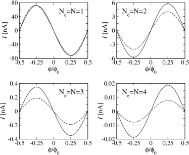
Figure 3: Persistent current in the insulating 1D ring as a function of magnetic flux for various ring lengths $N$. The ring is the periodic lattice with $N$ single-level potential wells (Fig. 2) which contains $N_{e}$ spinless electrons. It is insulating due to full filling ($N_{e}=N$). The full lines are the results of the LCAO formula (91) and the dashed lines are the results of the numerical LCAO approach. The ring parameters used in these calculations are specified in the caption of figure 2. The coefficients $\alpha_{j}$ and $\gamma_{j}$ in Eqs. (91) and (82) are given by expressions presented in appendix C.

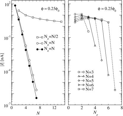
Figure 4: Persistent current in the same ring as in the preceding figure for magnetic flux $\phi=0.25\phi_{0}$. The left panel shows the dependence on $N$ for the insulating ring ($N_{e}=N$) and conducting ring at half filling ($N_{e}=N/2$). The right panel shows the dependence on $N_{e}$ for various values of $N$. In both panels, the data for $N_{e}=N$ shown by open symbols were obtained by means of the LCAO expression (91) and the data for partial filling ($N_{e}<N$) were obtained by means of expressions (1) and (2). The full circles in the left panel show the data for $N_{e}=N$, obtained using the numerical LCAO approach. Note that only the size of the current, $\mid I\mid$, is shown: for all presented data the sign of the current varies with varying parity of $N_{e}$.

Origin of all these differences is easy to see. Equations (1) and (2) depend only on the hopping amplitude $\Gamma_{1}$, while the result (91) is determined by the hopping amplitude $\Gamma_{N}$. The amplitude $\Gamma_{N}$ involves overlap of the Wannier functions $W_{l}(x)$ and $W_{l+N}(x)$. If we express the coefficient $c_{l^{\prime}-l}$ in equation (84) by means of equations (88) and (89), we obtain

$$W_{l}(x)\simeq\sum_{l^{\prime}=-\infty}^{\infty}\ \mid A_{\mid l^{\prime}-l\mid}\mid(-\alpha_{1})^{\mid l^{\prime}-l\mid}\mid\ \varphi_{a}(x-l^{\prime}a)\ .$$ (92)

If we keep $x=na$ and $l=0$ for simplicity, we obtain

$$W_{0}(na)\simeq\frac{1}{\sqrt{\pi\mid n\mid}}(-\alpha_{1})^{\mid n\mid}\varphi_{a}(0)\ ,\ \ \mid n\mid\geq 1\ .$$ (93)

It can be seen that the Wannier function decays with distance from site $l=0$ exponentially comment_Wannierfucntions and even shows the alternating sign for positive $\alpha_{1}$. All these properties are reflected by persistent current at full filling.

Finally, we calculate the persistent current quantitatively for the numerical parameters in figure 2. These parameters emulate the 1D GaAs ring modulated by a periodic lattice of $N$ quantum dots. In such lattice, the discrete energy level of the quantum dot splits into the energy band. Therefore, the ring behaves at full filling ($N_{e}=N$) like a band insulator and at partial filling ($N_{e}<N$) as a metal.

The figure 3 shows the persistent current in the insulating ring as a function of magnetic flux for various $N$. The results evaluated by means of the LCAO formula (91) are compared with the results obtained by the numerical LCAO approach. The numerical LCAO approach nicely confirms basic features of the formula (91) including the alternating sign of the current. The quantitative difference between the numerical and analytical LCAO data could be suppressed by choosing the ring with a more strongly localized atomic orbitals.

The dependence on the ring size is presented in figure 4. The left panel shows the persistent current as a function of $N$ in the insulating ring and in the conducting ring at half filling. The conducting ring shows for large $N$ the decay $I\propto 1/N$, in the insulating ring the current decays with $N$ exponentially. For example, the insulating ring with $N=5$ supports the persistent current as small as $\sim 0.001$nA. Such small persistent currents are detectable by sensitive techniques Bleszynski ; Bleszynski2 ; Bleszynski3 .

The right panel of figure 4 shows the transition from the conducting state to the insulating state at $N_{e}=N$, achieved by varying $N_{e}$ for fixed $N$. Experimentally, $N_{e}$ could be varied say by using a suitably designed metallic gate, while the quantum-dot lattice might be realized either by means of the periodic array of gates or by producing the 1D ring with a periodically alternating cross-section size.

VI VI. Estimates of persistent current in rings made of real band insulators

In the previous section, we have discussed the ring made of the artificial band insulator, namely the 1D GaAs ring with a few conduction electrons subjected to the periodic quantum-dot potential. Now we want to estimate persistent current in rings made of the real crystalline band insulators (with fully occupied valence band and empty conduction band). The problem is that such rings are three-dimensional and the 1D theory from the preceding text is not applicable directly.

Figure 5: The top figure shows the 3D ring (on the right hand side) created from the cubic 3D atomic lattice (on the left hand side) with the lattice period $a$. The ring of width $w$ is defined by two concentric circles with the center positioned at random. The resulting ring is a 3D cluster of atoms which can no longer be viewed as the 1D lattice with period $d$. The bottom figure shows the ring artificially linearized by means of elastic deformation. Repeating the linearized ring with period $L$ in the $x$ direction and with period $w$ in the $y$ direction, we obtain the infinite crystal. In the limit $L\gg w$ the effect of the elastic deformation has to disappear and the Bloch states in the obtained infinite crystal have to coincide with the electronic states in the real ring (top right sketch). This allows us to use the equations (94) and (95). We call this model the model of the linearized 3D cluster.

The problem is outlined in figure 5. The top right sketch in the figure is a 2D sketch of the 3D ring (or a hollow 3D cylinder) of width $w$, created from the cubic 3D lattice of atoms. Along such ring there is no periodicity with the lattice period $a$, there is only periodicity with $L$. However, the theory in Sects. III - V was developed for the 1D rings with periodicity $a$ along the ring circumference. The question is how to extend the 1D theory to be applicable to the ring-shaped 3D cluster of atoms sketched in the figure 5.

In principle, for $L\gg w$ it is reasonable to write the 3D version of equation (24) in the form

$$I(\phi)=-\frac{\partial}{\partial{\phi}}\sum_{n,k_{z}}\varepsilon_{n}(\phi,k_{y}=0,k_{z}),$$ (94)

with the spectrum of the ring, $\varepsilon_{n}(\phi,k_{y}=0,k_{z})$, determined as follows:

$$\varepsilon_{n}(\phi,k_{y}=0,k_{z})=\varepsilon(k_{x}=\frac{2\pi}{L}(n+\frac{\phi}{\phi_{0}}),k_{y}=0,k_{z}),$$ (95)

where $\varepsilon(k_{x},k_{y},k_{z})$ is the Bloch energy of the 3D crystal created by periodic repetition of the linearized 3D cluster (Fig.5). Note that the unit cell of the crystal is the linearized cluster. The Bloch energy $\varepsilon(k_{x},k_{y},k_{z})$ should therefore not be confused with the Bloch energy of the crystal with unit cell $a^{3}$. We call this approach the model of the linearized 3D cluster.

The model also allows to rewrite for 3D rings all equations of Sect. III. First of all, since the period $a$ along the ring no longer exists, it has to be replaced by the period $L$ (replace $a$ by $L$ and $N$ by unity). Second, the Bloch energy $\varepsilon(k_{x})$ has to be replaced by the Bloch energy $\varepsilon(k_{x},k_{y}=0,k_{z})$ just introduced. Third, the current (35) has to be summed over the occupied states $k_{z}$. Clearly, the model of the linearized 3D cluster allows to avoid a full 3D treatment of the ring-shaped 3D cluster. However, the model is still cumbersome for practical use because the Bloch spectrum $\varepsilon(k_{x},k_{y},k_{z})$ needs to be calculated for a nontrivial artificial crystal resulting from the periodic repetition of the linearized cluster.

Figure 6: The 3D ring of length $L$ and width $w$, created by elastic bending of the cubic 3D atomic lattice with lattice period $a$. In the limit $w\ll L$ the effect of the elastic bending has to disappear and the electronic states in such ring have to coincide with the Bloch states in the constituting 3D crystal as described in the text (equation 97). We call this model the model of the elastically bent 3D crystal. Obviously, the resulting 3D ring shows for $w\ll L$ an artificial periodicity with period $a$, which is not the case for the realistic 3D ring (fig. 5).

A more simple approach is to consider the artificial 3D ring obtained by elastic bending of the bulk crystal, as it is shown in figure 6. In this case we have instead of the formula (94) the formula

$$I(\phi)=-\frac{\partial}{\partial{\phi}}\sum_{n,k_{y},k_{z}}\varepsilon_{n}(\phi,k_{y},k_{z}),$$ (96)

where the energy spectrum $\varepsilon_{n}(\phi,k_{y},k_{z})$ is given by equation

$$\varepsilon_{n}(\phi,k_{y},k_{z})=\varepsilon(k_{x}=\frac{2\pi}{Na}(n+\frac{\phi}{\phi_{0}}),k_{y},k_{z}),$$ (97)

with $\varepsilon(k_{x},k_{y},k_{z})$ being the Bloch energy in the bulk crystal before it is bent. We call this approach the model of the elastically bent 3D crystal. In this model there is an artificial periodicity with period $a$ along the ring. In spite of this, the model can provide a reasonable quantitative information on how the persistent current in the 3D ring depends on the realistic band structure of the constituting bulk crystal. In the model, the persistent current at full filling is given by equations (47) and (46) modified as follows. The Bloch energy $\varepsilon(k_{x})$ in the Fourrier transformation (46) has to be replaced by the Bloch energy $\varepsilon(k_{x},k_{y},k_{z})$ and the current (47) should be summed over the occupied states $k_{y}$ and $k_{z}$. Practical calculations are relatively straightforward, because the Bloch spectrum of the bulk crystal, $\varepsilon(k_{x},k_{y},k_{z})$, is known for many insulators.

In what follows we apply the model of the elastically bent 3D crystal to the rings with thickness equal to the unit cell of the bulk crystal. The energy dispersion of the ring, $\varepsilon_{n}(\phi,k_{y}=0,k_{z}=0)$, is extracted from the bulk crystal dispersion $\varepsilon(k_{x},k_{y}=0,k_{z}=0)$, calculated by microscopic methods Chadi-Cohen ; Loehr . The obtained persistent current should be viewed as a minimum value estimate, because the thickness of realistic rings is much larger than the unit cell.

Figure 7: The panels in the right column show the valence bands of various band insulators like the GaAs, Ge, and InAs. Specifically, the $\epsilon(k)$ dispersion curves of the light-hole band (full line), double-degenerate heavy-hole band (dashed line), and lowest band (dotted line) are plotted for the $k$-values on the line ($L[-\pi/a,-\pi/a,-\pi/a],\Gamma[0,0,0],L[\pi/a,\pi/a,\pi/a]$). The panels in the left column show the hopping amplitude $\Gamma_{N}$, calculated separately for each band: the $\epsilon(k)$ dependence of the band is Fourier-transformed by using the equation (46). The full, dashed, a dotted lines show $\Gamma_{N}$ for the light-hole, heavy-hole, and lowest bands, respectively. When compared with $\Gamma_{N}$ of the light-hole and heavy-hole band , $\Gamma_{N}$ of the lowest band has opposite sign because of the opposite curvature of the $\epsilon(k)$ curve and the presented data should be multiplied by $-1$ as shown in the figure (but see the comment comment1 ).

Using standard methods Chadi-Cohen ; Loehr , in the figure 7 we numerically reproduce the well-known band structure of the band insulators like the GaAs, Ge, and InAs. Specifically, the figure summarizes the $\epsilon_{k}$ curves of the light-hole band, heavy-hole band and lowest band, calculated for the line ($L[-\pi/a,-\pi/a,-\pi/a],\Gamma[0,0,0],L[\pi/a,\pi/a,\pi/a]$) in the first Brillouin zone. We set each of these $\epsilon(k)$ curves numerically into the Fourier transformation (46) and we calculate for each band the hopping amplitude $\Gamma_{N}$. The resulting $\Gamma_{N}$ dependencies are shown in the figure 7.

By means of the figure 7 we estimate the persistent current as follows. We form the ring by elastic bending of the crystal. We choose the ring orientation for which the $k$ states on the line ($L[-\pi/a,-\pi/a,-\pi/a],\Gamma[0,0,0],L[\pi/a,\pi/a,\pi/a]$) are directed along the ring circumference. If the ring is one-dimensional (with thickness equal to a single unit cell of the crystal), the persistent current is given by the 1D formula (47) with the hopping amplitude $\Gamma_{N}$ given by numerical values in the figure 7. As expected, $\Gamma_{N}$ decays with increasing $N$ exponentially, however, for the light-hole band the decay is much slower than for other two bands. Therefore it is sufficient to calculate the persistent current in the light-hole band. The results are shown in the figure 7. We recall that these results represent the persistent current carried by electrons in the fully occupied valence band. The following features are worth to point out.

The persistent current in the insulating ring decreases with the increasing ring length exponentially, but a careful choice of the insulating material allows to achieve the persistent current of measurable value for a technologically realizable ring size. Indeed, the maximum ring lengths considered in the figure 8 are close to the value $\sim 120$nm, in principle achievable by modern nanotechnology. Concerning the amplitude of the persistent current, the value $\sim 0.0003$nA estimated for the InAs ring of length $\sim 120$nm is very small, but in principle detectable say by the experimental technique of Refs. Bleszynski ; Bleszynski2 ; Bleszynski3 . The considered insulators are ordered as GaAs, Ge and InAs for the persistent currents ordered increasingly. This suggests a simple rule: the smaller the light-hole effective mass the larger the persistent current.

We conclude with a few remarks showing that the above 1D estimates hold roughly also for the 3D rings. Similar calculations as in the figure 7 were performed for the $k$ values on the line ($X[-2\pi/a,0,0],\Gamma[0,0,0],X[2\pi/a,0,0]$). We have found the energies $\epsilon(k)$ and amplitudes $\Gamma_{N}$ (not shown) very similar to those in the figure 7, with the resulting persistent currents being of the same order of magnitude as those in the figure 8. Moreover, we have observed similar results when testing the $k$ values on the lines ($K,\Gamma,K$) and ($W,\Gamma,W$). The model of the elastically bent crystal thus provides roughly the same persistent current independently on the fact which crystalline axis is chosen to be directed along the ring circumference. This suggests that anisotropy of the valence band with respect to the $\vec{k}$ direction does affect the resulting persistent current dramatically. Therefore, the estimated values of the current should hold reasonably also for the realistic ring-shaped crystals similar to the ring sketched in figure 5.

Figure 8: Persistent current versus the ring length $N$ in the ring made of the real crystalline band insulator (GaAs, Ge, InAs). The persistent current is estimated by means of the 1D formula (47), where $\Gamma_{N}$ is the hopping amplitude of the electron in the light-hole band, calculated in the preceding figure. The lattice constants of the GaAs, Ge, and InAs crystals are $\sim 0.6$nm, i.e., the maximum ring lengths considered in the figure are $L=Na\sim 120$nm. The rings of such length could be realizable by means of advanced nanotechnology.

VII VII. Summary and concluding remarks

We have analyzed theoretically persistent currents in rings made of band insulators. We started by formulating a recipe which determines the Bloch states of a one-dimensional (1D) ring from the Bloch states of an infinite 1D crystal created by the periodic repetition of the ring. Using the recipe, we have derived an expression for the persistent current in a 1D ring made of an insulator with an arbitrary valence band $\epsilon(k)$.

To find an exact result for a specific insulator, we have considered a 1D ring represented by a periodic lattice of $N$ identical sites with a single value of the on-site energy. If the Bloch states in the ring are expanded over a complete set of $N$ on-site Wannier functions, the discrete on-site energy splits into the energy band. At full filling, the band emulates the valence band of the band insulator and the ring is insulating.

We have found that the ring carries a persistent current equal to the product of $N$ and the derivative of the on-site energy with respect to the magnetic flux. This current is not zero because the on-site Wannier function and consequently the on-site energy of each ring site depend on magnetic flux.

Further, we have expanded all $N$ Wannier functions of the ring over the basis of Wannier functions of the constituting infinite 1D crystal. In terms of the crystal Wannier functions, the current at full filling arises because the electron in the ring with $N$ lattice sites is allowed to make a single hop from site $i$ to its periodic replicas $i\pm N$. Alternatively, in terms of the ring Wannier functions the same current is due to the flux dependence of the Wannier functions basis, and the longest allowed hop is from $i$ to $i\pm{\rm Int}(N/2)$ only.

We have eventually derived the crystal Wannier functions in the LCAO approximation, and have expressed the persistent current at full filling by means of an exact formula. The validity of the formula was verified by comparison with the numerical LCAO approach. We have presented quantitative results for a 1D ring made of an artificial band insulator, namely for a GaAs ring subjected to a periodic potential emulating the insulating lattice.

Moreover, we have provided estimates for the rings made of real band insulators (GaAs, Ge, InAs) with a fully filled valence band and empty conduction band. The current at full filling decays with the ring length exponentially due to the exponential decay of the Wannier function tails. In spite of that, it can be of measurable size.

We have ignored the effect of nonzero temperature. We expect the persistent currents in rings made of the band insulators to be temperature-independent as long the thermal energy $k_{B}T$ is much smaller than the energy gap separating the valence band from the conduction band. For example, the energy gap in the InAs crystal is $\sim 400$meV. Hence, the zero-temperature values of the persistent current, predicted for the insulating InAs ring, could persist even at room temperature.

We have also ignored the electron-electron interaction. The many-body studies Mosko-PRB ; Nemeth-PRB suggest that in the 1D ring considered in this paper the repulsive electron-electron interaction would only renormalize the electron transmission through the potential barrier separating two potential wells. That means that the electron-electron interaction would not essentially change our results.

Finally, we relate our results to the paper by Kohn Kohn1 , which defines the insulating state as a property of the many-body ground state (see also the review by Resta Resta ). Kohn’s paper contains a discussion implicitly admitting the existence of a negligibly small persistent current in the insulating ring [see the discussion of equations (2.23) - (2.31) in that work]. Kohn points out the exponential localization of the electron states in the ring. However, he clearly states by writing his equation (2.30), that the current is zero only approximately. Just this negligibly small current is calculated in our paper. Surprisingly, it can be of measurable size.

VIII Acknowledgements

This work was supported by grants APVV-51-003505 and VVCE-0058-07 from the Grant Agency APVV and by grants VEGA-2/0633/09 and VEGA-2/0206/11 from the Grant Agency VEGA. We thank Pavol Quittner for important help with the mathematical derivation in Appendix D.

IX Appendix A: Derivation of equation (30) from equation (28)

We start by writing Eq. (28) as

$$\varepsilon_{n}(\phi)=\sum_{j^{\prime}=0}^{\infty}a_{j^{\prime}}\cos\left(k_{n}(\phi)\ j^{\prime}a\right)\ ,$$ (98)

Using substitution $j^{\prime}=Ns+j$, where $s=0,1,2,\dots$ and $j=0,1,\dots(N-1)$, we obtain

$$\varepsilon_{n}(\phi)=\sum_{j=0}^{N-1}\sum_{s=0}^{\infty}a_{sN+j}\cos\left[k_{n}(\phi)(sN+j)a\right].$$ (99)

Assuming that $N$ is odd we rewrite Eq. (99) as

$$\varepsilon_{n}(\phi) = \sum_{s=0}^{\infty}a_{sN}\cos\left[k_{n}(\phi)sNa\right]$$

$$+ \sum_{j=1}^{M}\sum_{s=0}^{\infty}a_{sN+j}\cos\left[k_{n}(\phi)(sN+j)a\right]$$

$$+ \sum_{j=M+1}^{N-1}\sum_{s=0}^{\infty}a_{sN+j}\cos\left[k_{n}(\phi)(sN+j)a\right]\ ,$$

where $M={\rm Int}(N/2)$. Equation (LABEL:e_k_n1) can be rewritten as

$$\varepsilon_{n}(\phi) = \sum_{s=0}^{\infty}a_{sN}\cos\left[k_{n}(\phi)sNa\right]$$

$$+ \sum_{j=1}^{M}\sum_{s=0}^{\infty}\Bigl{\{}a_{sN+j}\cos\left[k_{n}(\phi)(sN+j)a\right]\Bigr{.}$$

$$+ \Bigl{.}a_{(sN+N-j)}\cos\left[k_{n}(\phi)\left(sN+N-j\right)a\right]\Bigr{\}}\ .$$

Utilizing definition (29) we find from Eq. (IX) the result

$$\varepsilon_{n}(\phi)=\Omega_{0}+\sum_{j=1}^{M}\Bigl{\{}\Omega^{R}_{j}\cos\left(k_{n}(\phi)\ ja\right)+\Omega^{I}_{j}\sin\left(k_{n}(\phi)\ ja\right)\Bigr{\}}\ ,$$ (101)

where

$$\Omega_{0}(\phi)=\sum_{s=0}^{\infty}a_{sN}\ \cos(2\pi\frac{\phi}{\phi_{0}}s)\ ,$$

$$\Omega^{R}_{j}(\phi)=a_{j}+\sum_{s=1}^{\infty}\ \cos(2\pi\frac{\phi}{\phi_{0}}s)\left[a_{sN+j}+a_{sN-j}\right]\ ,$$

$$\Omega^{I}_{j}(\phi)=\sum_{s=1}^{\infty}\ \sin(2\pi\frac{\phi}{\phi_{0}}s)\left[a_{sN-j}-a_{sN+j}\right]\ .$$

(102)

We have sofar assumed odd $N$. For even $N$, derivation is similar and we find again the results (101) and (102), except that for $j=N/2$ we have instead of Eqs. (102) the equations

$$\Omega^{R}_{N/2}(\phi)=\sum_{s=0}^{\infty}\ a_{sN+N/2}\ \cos(2\pi\frac{\phi}{\phi_{0}}s)\ ,$$

$$\Omega^{I}_{N/2}(\phi)=-\sum_{s=1}^{\infty}\ a_{sN+N/2}\sin(2\pi\frac{\phi}{\phi_{0}}s)\ .$$

(103)

Equation (101) coincides with Eq. (30).

X Appendix B: Various forms of equation (60)

We first assume odd $N$. We can rewrite Eq. (60) as

$$\varepsilon_{n}(\phi)=T_{0}+\sum_{j=1}^{M}\ e^{-i{k_{n}(\phi)}ja}T_{j}+\sum_{j=M+1}^{N-1}e^{-i{k_{n}(\phi)}ja}T_{j},$$ (104)

where $M=\rm Int(N/2)$. Further,

$$\varepsilon_{n}(\phi) = T_{0}+\sum_{j=1}^{M}\ e^{-i{k_{n}(\phi)}ja}T_{j}+\sum_{j=1}^{M}e^{-i{k_{n}(\phi)}(N-j)a}T_{N-j}$$

$$= T_{0}+\sum_{j=1}^{M}\ e^{-i{k_{n}(\phi)}ja}T_{j}+e^{i{k_{n}(\phi)}ja}T^{*}_{j}\ ,$$

where we have used the definition (29) and relations

$$T^{*}_{j}=T_{-j}\ ,\quad\quad T_{N-j}=e^{i2\pi\frac{\phi}{\phi_{0}}}T^{*}_{j}\ ,$$ (106)

which follow from Eq. (59) for real $\varepsilon_{n}(\phi)$. For even $N$ we obtain in a similar way the equation

$$\varepsilon_{n}(\phi) = T_{0}+\sum_{j=1}^{M-1}\ e^{-i{k_{n}(\phi)}ja}T_{j}+e^{i{k_{n}(\phi)}ja}T^{*}_{j}$$

$$+ e^{-i{k_{n}(\phi)}\frac{N}{2}a}T_{\frac{N}{2}}\ .$$

Equations (LABEL:eigenenergy4) and (LABEL:eigenenergy42) can be written in the unified form

$$\varepsilon_{n}(\phi)=\Lambda_{0}+\sum_{j=1}^{M}\Bigl{\{}\Lambda^{R}_{j}\cos\left(k_{n}(\phi)\ ja\right)+\Lambda^{I}_{j}\sin\left(k_{n}(\phi)\ ja\right)\Bigr{\}}\ ,$$ (108)

where

$$\Lambda_{0}=T_{0}\ ,$$

$$\Lambda^{R}_{j}=(T_{j}+T^{\ast}_{j})\ ,$$

$$\Lambda^{I}_{j}=\frac{1}{i}(T_{j}-T^{\ast}_{j})\$$

(109)

for odd $N$ as well as even $N$, except that for even $N$ and $j=N/2$ we have instead of equations (109) the equations

$$\Lambda^{R}_{N/2}=\frac{1}{2}(T_{j}+T^{\ast}_{j})\ ,$$

$$\Lambda^{I}_{N/2}=\frac{1}{2i}(T_{j}-T^{\ast}_{j})\ .$$

(110)

Equation (108) is formally equivalent with Eq. (101). Coincidence of both equations becomes obvious if we realize that equations (109) and (110) coincide with Eqs. (102) and (103). To observe this coincidence, it is sufficient to express $T_{j}$ in equations (109) and (110) by means of expression (68), and to use the equations $a_{0}=\Gamma_{0}$ and $a_{j}=2\Gamma_{j}$.

XI Appendix C: Analytical formulas for $\alpha_{j}$ and $\gamma_{j}$

For the square-well potential in figure 1 the atomic orbitals $\varphi_{a}(x-la)$ can be found easy and the integrals (79) and (80) can be calculated analytically. For $j=1,2,\dots$ we obtain

$$\alpha_{j}\simeq\frac{\cos^{2}(Ad)}{1+Bd}e^{-B(ja-2d)}\left[\frac{-4\epsilon_{a}}{V_{0}}+B(ja-2d)\right]\ ,$$ (111)

$$\gamma_{j}\simeq V_{0}\frac{\cos^{2}(Ad)}{1+Bd}e^{-B(ja-2d)}\left[\frac{-2\epsilon_{a}}{V_{0}}+2dB(j-1)\right]\ ,$$ (112)

where

$$A=\sqrt{\frac{2m}{\hbar^{2}}\left(V_{0}+\epsilon_{a}\right)},\quad\quad B=\sqrt{\frac{2m}{\hbar^{2}}\left|\epsilon_{a}\right|}.$$ (113)

In addition, for $j=0$

$$\gamma_{0}=V_{0}\frac{\cos^{2}(Ad)}{1+Bd}e^{-2B(a-2d)}\frac{1-e^{-4Bd}}{1-e^{-2Ba}}\ .$$ (114)

Expressions (111) and (112) are not exact (we have skipped some exponentially small terms), but they are in excellent agreement with numerical integration of the integrals (79) and (80). As expected, the coefficients $\alpha_{j}$ and $\gamma_{j}$ decay with increasing $j$ exponentially. The simplest forms are

$$\gamma_{j}\simeq\gamma_{1}\ e^{-(j-1)Ba}\ ,\ \ \ \alpha_{j}\simeq\alpha_{1}\ e^{-(j-1)Ba}\ ,\ \ \ j\geq 1\ .$$ (115)

XII Appendix D: Approximate formulas for coefficients $c_{n}$ and $\Gamma_{j}$

Equation (85) defines $c_{n}$ by means of the integral which can be calculated analytically in a certain limit. In what follows the calculation is presented for positive $n$ because $c_{n}=c_{-n}$. We first express the normalization constant $\frac{1}{\sqrt{N(k)}}$ as

$$\frac{1}{\sqrt{N(k)}} = \left[1+2\sum_{j=1}^{\infty}\alpha_{j}\cos jka\right]^{-\frac{1}{2}}$$ (116)

$$= \sum_{s=0}^{\infty}\ A_{s}\left[2\sum_{j=1}^{\infty}\alpha_{j}\cos jka\right]^{s}\ ,$$

where

$$A_{s}=(-1)^{s}\frac{1}{2^{2s}}\ \binom{2s}{s}\ .$$ (117)

A closer inspection of the right hand side of Eq. (116) shows, that the equation (116) can be approximated as

$$\frac{1}{\sqrt{N(k)}}\simeq\sum_{s=0}^{\infty}\ A_{s}\left[2\alpha_{1}\cos ka\right]^{s}\ ,$$ (118)

if $\alpha_{j}$ falls with $j$ exponentially as in equation (115), and if $\alpha_{1}^{2}\gg\alpha_{2}$. We note that the latter condition takes the form $\alpha_{1}\gg\exp(-Ba)$ for $\alpha_{j}$ derived in the preceding appendix. In general, both conditions are fulfilled simultaneously if the localization of the atomic orbitals is strong enough in comparison with the lattice constant $a$.

We set the expansion (118) into the formula (85) and we perform the integration. We get

$$c_{n}\simeq\sum_{s=0}^{\infty}\ A_{s}\left[2\alpha_{1}\right]^{s}\ I_{n,s}\ ,$$ (119)

where

$$I_{n,s}=\frac{1}{\pi}\int_{-{\pi}}^{{\pi}}\cos(nx)\cos^{s}(x)dx\ .$$ (120)

It can be seen that

$$I_{n,s}=0\ ,$$ (121)

if $s<n$ or if $(s-n)$ is odd. It can also be seen that

$$I_{n,s}=\frac{2}{2^{n+2l}}\ \binom{n+2l}{l}\ ,$$ (122)

if $s=n+2l$, where $l=0,1,\dots$ .

We set equations (122) and (121) into the equation (119). We get an approximate expression for $c_{n}$,

$$c_{n}=\left(-\alpha_{1}\right)^{n}\sum_{l=0}^{\infty}\ A_{n+2l}\ \alpha_{1}^{2l}\ \binom{n+2l}{l}\ .$$ (123)

The last equation can be further rewritten as

$$c_{n} = \left(-\alpha_{1}\right)^{n}\left|A_{n}\right|\sum_{l=0}^{\infty}\ \frac{A_{n+2l}}{A_{n}}\ \alpha_{1}^{2l}\ \binom{n+2l}{l}$$ (124)

$$< \left(-\alpha_{1}\right)^{n}\left|A_{n}\right|\sum_{l=0}^{\infty}\alpha_{1}^{2l}\ \binom{n+2l}{l}\ ,$$

where the right hand side is a properly chosen upper limit (because $A_{n+2l}/A_{n}<1$).

If we use the relation

$$\sum_{l=0}^{\infty}(\alpha_{1}^{2})^{l}\binom{n+2l}{l}=\frac{1}{\sqrt{1-4\alpha_{1}^{2}}}\left(\frac{2}{1+\sqrt{1-4\alpha_{1}^{2}}}\right)^{n}\ ,$$ (125)

the inequality (124) reads

$$c_{n}<\left(-\alpha_{1}\right)^{n}\left|A_{n}\right|\frac{1}{\sqrt{1-4\alpha_{1}^{2}}}\left(\frac{2}{1+\sqrt{1-4\alpha_{1}^{2}}}\right)^{n}\ .$$ (126)

For $\alpha_{1}\ll 1/2$ it can be further approximated as

$$c_{n}<\left(-\alpha_{1}\right)^{n}\left|A_{n}\right|\left(1+\alpha_{1}^{2}\right)^{n}$$ (127)

We return again to the equation (123) and we replace its right hand side by a properly chosen lower limit:

$$c_{n} > \left(-\alpha_{1}\right)^{n}\left|A_{n}\right|\sum_{l=0}^{n}\binom{n}{l}\left(\alpha_{1}\right)^{2l}$$

$$> \left(-\alpha_{1}\right)^{n}\left|A_{n}\right|\left(1+\alpha_{1}^{2}\right)^{n}\ ,$$

where we have utilized the inequality

$$\frac{A_{n+2l}}{A_{n}}\binom{n+2l}{l}>\binom{n}{l}\ .$$ (129)

Notice now that the right hand sides of the inequalities (127) and (LABEL:wanier_coeficient_down) coincide. This implies that

$$c_{n}=\left(-\alpha_{1}\right)^{n}\left(1+\alpha_{1}^{2}\right)^{n}\left|A_{n}\right|\simeq\left(-\alpha_{1}\right)^{n}\left|A_{n}\right|\ .$$ (130)

Now we attempt to find an approximate expression for the coefficient ${\it\Gamma}_{j}$. Equation (86) can be rewritten by means of substitution $n^{\prime}-n=m$ as

$${\it\Gamma}_{j}=\sum_{m=-\infty}^{\infty}\ (\varepsilon_{a}\alpha_{m}-\gamma_{m})\sum_{n=-\infty}^{\infty}c_{n}c_{j+m+n}\ .$$ (131)

Since $c_{n}=c_{-n}$ , $\alpha_{n}=\alpha_{-n}$, and $\gamma_{n}=\gamma_{-n}$, we obtain

$${\it\Gamma}_{j} =\left(\varepsilon_{a}\alpha_{0}-\gamma_{0}\right)\Bigl{[}c_{0}c_{j}+\sum_{n=1}^{\infty}c_{n}\left(c_{j+n}+c_{j-n}\right)\Bigr{]}$$

$$+ \sum_{m=1}^{\infty}\left(\varepsilon_{a}\alpha_{m}-\gamma_{m}\right)\Bigl{[}c_{0}\left(c_{j+n}+c_{j-n}\right)\Bigr{.}$$

$$+ \Bigl{.}\sum_{n=1}^{\infty}c_{n}\left(c_{j+m+n}+c_{j+m-n}+c_{j-m+n}+c_{j-m-n}\right)\Bigr{]}\ .$$

Owing to the exponential dependence (130), the last equation can be simplified as

$$\Gamma_{j}\simeq\sum_{m=0}^{j}\left(\varepsilon_{a}\alpha_{m}-\gamma_{m}\right)\sum_{n=0}^{j-m}c_{n}c_{j-m-n}\ .$$ (133)

Setting for $c_{n}$ and $A_{n}$ the equations (130) and (117) we have

$$\Gamma_{j}\simeq\sum_{m=0}^{j}\left(\varepsilon_{a}\alpha_{m}-\gamma_{m}\right)\left(-\alpha_{1}\right)^{j-m}\ .$$ (134)

Expressing $\gamma_{n}$ and $\alpha_{n}$ by means of the equation (115) we further obtain

$$\Gamma_{j} \simeq \left(\varepsilon_{a}-\gamma_{0}\right)\left(-\alpha_{1}\right)^{j}$$

$$+ \sum_{m=1}^{j}\left(\varepsilon_{a}\alpha_{1}-\gamma_{1}\right)e^{-(m-1)Ba}\left(-\alpha_{1}\right)^{j-m}\ .$$

If $\alpha_{1}\gg\exp(-Ba)$, we can skip all terms with $m\geq 2$. Thus

$${\it\Gamma}_{j}\simeq\left(-\alpha_{1}\right)^{j-1}\left[-\gamma_{1}+\gamma_{0}\alpha_{1})\right]\simeq-\left(-\alpha_{1}\right)^{j-1}\ \gamma_{1}\ .$$ (136)

References

• (1) Y. Imry, Introduction to Mesoscopic Physics (Oxford University Press, Oxford, UK, 2002).
• (2) N. Byers and C.N. Yang, Phys. Rev. Lett. 7, 46 (1961).
• (3) F. Bloch, Phys. Rev. 137, A787 (1965); 166,415 (1968).
• (4) M. Büttiker, Y. Imry, and R. Landauer, Phys. Lett. A 96, 365 (1983).
• (5) L. P. Lévy, G. Dolan, J. Dunsmuir, and H. Bouchiat, Phys. Rev. Lett. 64, 2074 (1990).
• (6) V. Chandrasekhar, R. A. Webb, M. J. Brady, M. B. Ketchen, W. J. Gallagher, and A. Kleinsasser, Phys. Rev. Lett. 67, 3578 (1991).
• (7) E. M. Q. Jariwala, P. Mohanty, M. B. Ketchen, and R. A. Webb,  Phys. Rev. Lett. 86, 1594 (2001).
• (8) H. Bluhm, N. C. Koschnick, J. A. Bert, M. E. Huber, and K. A. Moler, Phys. Rev. Lett. 102, 136802 (2009).
• (9) A. C. Bleszynski-Jayich, W. E. Shanks, B. Peaudecerf, E. Ginossar, F. von Oppen, L. Glazman, and J. G. E. Harris, Science 326, 272 (2009).
• (10) D. Mailly, C. Chapelier, A. Benoit, Phys. Rev. Lett. 70, 2020 (1993).
• (11) W. Rabaud, L. Saminadayar, D. Mailly, K. Hasselbach, A. Benoît, B. Etienne,  Phys. Rev. Lett. 86, 3124 (2001).
• (12) U. Eckern, and P. Schwab, J. Low Temp. Phys. 126, 1291 (2002).
• (13) L. Saminadayar, C. Bauerle, and D. Mailly, Encycl. Nanosci. Nanotech. 3, 267 (2004).
• (14) J. Feilhauer and M. Moško, Phys. Rev. B 84, 085454 (2011).
• (15) M. Moško, unpublished (2006).
• (16) H.-F. Cheung, Y. Gefen, E. K. Riedel, W.-H. Shih, Phys. Rev. B 37, 6050 (1988).
• (17) W. Kohn, Phys. Rev. 133, A171 (1964).
• (18) A. Mošková, M. Moško, and A. Gendiar, Physica E, 1991 (2008).
• (19) R. Németh, M. Moško, Physica E 40, 1498 (2008).
• (20) M. A. Pinsky, Introduction to Fourier Analysis and Wavelets, (American Mathematical Society, 2002).
• (21) N. W. Ashcroft, and N. D. Mermin, Solid state physics, Sounders College Publishing, Ed. D. G. Crane, Cornell University, USA 1976.
• (22) W. Kohn, Phys. Rev. B 7, 4388 (1973).
• (23) W. Andreoni, Phys. Rev. B 14, 4247 (1976).
• (24) Precisely, equation (93) shows the decay ${\mid n\mid}^{-1/2}{\mid\alpha_{1}\mid}^{\mid n\mid}$. A purely exponential decay was predicted by W. Kohn, Phys. Rev. 115, 809 (1959). A very sophisticated estimates by L. He and D. Vanderbilt, Phys. Rev. Lett. 86, 5341 (2001), and by A. Bruno-Alfonso and D. R. Nacbar, Phys. Rev. B 75, 115428 (2007), predict (in our notations) the decay ${\mid n\mid}^{-3/4}{\mid\alpha_{1}\mid}^{\mid n\mid}$. For our purposes, exact nature of the power law prefactor is of minor importance.
• (25) A. C. Bleszynski-Jayich, W. E. Shanks, and J. G. E. Harris, Appl. Phys. Lett 92, 013123 (2008).
• (26) A. C. Bleszynski-Jayich, W. E. Shanks, R. Ilic, and J. G. E. Harris, J. Vac. Sci.Technol  26, 1412 (2008).
• (27) In fact, the details of the $\Gamma_{n}$ dependence of the lowest band are not essential for the resulting persistent current since the dominant contribution to the current is due to the light-hole band (see the text). We note only for completeness that in the GaAs and InAs the $\Gamma_{N}$ dependence of the lowest band exhibits the same sign for all $N$ except for a few isolated values of $N$ where the sign is opposite. We plot the whole $\Gamma_{N}$ curve of the lowest band with a fixed sign for simplicity. Due to this simplification the $\Gamma_{N}$ curve exhibits a few local minima: the $\Gamma_{N}$ values at these minima in fact do not have the same sign as the rest of the curve.
• (28) D.J. Chadi and M.L. Cohen, Phys. Status Solidi B 68, 405 (1975).
• (29) J. P. Loehr, and D. N. Talwar, Phys. Rev. B 55, 4353 (1997).
• (30) M. Moško, R. Németh, R. Krčmár, and M. Indlekofer, Phys. Rev. B 79, 245323 (2009).
• (31) R. Németh, M. Moško, R. Krčmár, A. Gendiar, K. M. Indlekofer, and L. Mitas, arXiv:0902.2225 (2009).
• (32) R. Resta, Eur. Phys. J. B 79, 121 (2011).