A simple strategy for renormalization: QED at one-loop level

Abstract

We demonstrate our simple strategy for renormalization with QED at one-loop level, basing on an elaboration of the effective field theory philosophy. No artificial regularization or deformation of the original theory is introduced here and hence no manipulation of infinities, ambiguities arise instead of infinities. Ward identities first come to reduce the number of ambiguities, the residual ones could in principle be removed by imposing physical boundary conditions. Renormalization group equations arise as ”decoupling theorems” in the underlying theory perspective. In addition, a technical theorem concerning routing of external momenta is also presented and illustrated with the self-energy and vertex function as examples.

I Introduction

All the presently known quantum field theories for practical use are beset with ultraviolet divergences to certain extent in perturbative frameworks. These divergences imply that such theories are not well defined at short distances before renormalization is carried out, at least within perturbative frameworks. The celebrated BPHZ program is the standard algorithm for renormalizationBPHZ1 ; BPHZ2 ; BPHZ3 that is widely employed by particle and field theorists, which can lead to a mathematically well-defined perturbative formulation of a field theory in the end. But the procedures involved are not easy to be endowed with a natural logic that would be readily to accept. In this connection, Epstein and Glaser (EG) had already shown that finite perturbation theory of quantum field theories can be obtained through constructive methods basing on causality conditionsEG1 ; EG2 where Feynman rules are only valid at tree level, which provides more mathematical rationales for conventional procedures like BPHZEGBP1 ; EGBP2 . Recently, other mathematical structures hidden in the perturbative formulation (especially in BPHZ) of quantum field theories has become a rapidly growing area of researchHopf1 ; Hopf2 ; Hopf3 , which implies that there are more regularities worth exploring under the veil of renormalization.

From more physical point of view, according to the effective theory philosophy, the appearance of ultraviolet divergences can be understood from the fact that the presently known formulation of a quantum field theory is necessarily an effective one with the sophisticated structures or parameters dominant at short distances or larger energy scales being ignored. Unfortunately, the sophisticated structures underlying the present formulation of quantum field theories are actually unavailable or not discovered yet. Nor could us simply guess about the exact answers. The divergences or the ill-defined objects are the prices we paid for such forced ignorance or simplification. This is the start of the effective field theory philosophy that is now widely accepted and applied by physicists. Fortunately, this effective field theory view also implies that the ignored short-distance details could at best affect the physical behaviors of effective field theories through local interactions or operators that could be parametrized as corrections to the actions of quantum field theories, which, after being absorbed into the normalization factors for effective field theory’s couplings and operators, leads to the renormalization of quantum (effective) field theories. Otherwise they would be ”captured” as explicit and active degrees of freedom.

In practical computations, one usually has to first introduce various regularization schemes and intermediate divergences to be removed later, which are supposed to imitate the roles played by the true underlying structures or parameters. Actually, with such operations, the perturbative expansion only takes rather formal meaning due to the presence of infinite counter-terms. Moreover, for the regularization schemes or deformations to be legitimate and useful, they must not harm the bulk structures of the original theory as well as being self-consistent. In particular, important symmetries and global properties like the topologies of spacetime and Hilbert space, unitarity and causality, etc., which serve as foundations for a quantum field theory, should be preserved as much as possible, at least no drastic or uncontrollable changes should be introduced. However, the status of the principles just stated are extremely hard to precisely or profoundly assess within any known regularization. As a matter of fact, the comprehensive and global structures of a well-defined quantum field theory have never been fully delineated, and we heavily rely on rather formal evaluations to deal with this very difficult issue. Sometimes, to pursue efficiency, even the logical foundations of the theory would be severely mutilatedvisser . Thus, we only accumulate our faiths in one regularization method through intensive tests against experiment data. Up till now, there exists no regularization that could be satisfactorily in service in all contexts, each has certain shortcomings that will fail somewhere, or alternatively, no one could prove to work everywhere. For example, the celebrated dimensional regularization works excellently for standard model, especially for the strong interaction, but not for supersymmetric theories at allthooft1 ; thooft2 ; thooft3 ; thooft4 ; thooft5 ; thooft6 ; thooft7 ; thooft8 . Of course, other schemes also have their own shortcomings, for a comprehensive discussions of the advantages and disadvantages of various existing regularization methods, please refer to Ref.WuYL . This is also an indirect reflection of our ignorance of the grand structures or contents of quantum field theories in depth. Therefore, most regularization schemes are actually used in a superficial or formal sense, only appearing in the intermediate stages of calculations. After the artificial and transient excursion to parametrize our ignorance of the underlying short-distance physics, we ”return” to our ”original” quantum field theories with the deformations removed somehow. This practice is quite established within perturbative regimes for many physically interested quantities or operators. Nevertheless, the ultimate theoretical values for such doings still remain to be seen, at least in nonperturbative regimes.

On account of the above reasonings, it is definitely desirable or worthwhile to explore of any approach or procedure that would introduce no or as less as possible deformation of the bulk aspects of a quantum field theory and the associated infinities or divergences. For physicists, it is also more convenient to work with Feynman rules and Feynman diagrams that are physically intuitive and well defined at tree level in such a manner that the radiative corrections or loop diagrams could be computed without introducing too much mathematical auxiliaries. Actually, as will be demonstrated and argued below, there may exist an approach or strategy that seems to be free of the problems mentioned above or satisfy the requirements just enumerated. It is actually based on an elaboration of the effective field theory philosophytalk10 ; talk11 ; talk2 ; 981 ; 982 , introducing no artificial deformations, and more pleasantly, no ultraviolet infinities and the associated subtraction of infinities. Only local ambiguities for each loop integral may occur as a parametrization of our ignorance, which, as in the last step of renormalization, are to be fixed through appropriate boundary conditions. We feel all these virtues should make our strategy a simple and natural approach to start with. It has already been partially employed in a number of field theoretical issuesActa951 ; Acta952 ; PRD65 ; PRC71 ; SciChn .

From this report on, we wish to launch serial works to demonstrate, explain and further develop our strategy, with our ultimate goals targeting at a consistent and efficient program. In the course of these works, we will illustrate through concrete examples that many technical subtleties such as external momenta routing (or shift of integration variables) and overlapping divergent diagrams do not cause any trouble. From our demonstrations, one could find that our strategy could be well applied beyond the standard perturbative framework in terms of Feynman diagrams, see the applications in nonperturbative problemsPRC71 ; SciChn , unlike those principally devised for and limited to relativistic perturbative formulation. Another virtue of our approach is that we may examine important issues such as symmetry status of the radiative corrections (perturbative or nonperturbative) without being stuck to some specific prescription that might lead us to wrong conclusions or judgementActa951 ; Acta952 ; PRD65 . For perturbative amplitudes, our strategy could reproduce the EG approach’s results. In fact, our physically motivated strategy share the following consensus with the mathematically motivated EG approach: the perturbative quantum field theories are not unambiguously defined in the short distances, some elementary Feynman or loop diagrams contain local ambiguous terms that could only be fixed through appropriate boundary conditions. In this report, we employ the simple and well-known objects in quantum electrodynamics (QED) for a clear and pedagogical illustration of the ”naturalness” and simplicity of the principles and perspective that are adopted in our approach. In a sense, we wish to motivate an elaboration of the effective field theories philosophy with respect to renormalization of all quantum processes.

The organization of this report is as follows: We describe our strategy in Sec. II along with some technical issues. In Sec. III, we compute the elementary one-loop amplitudes or Feynman graphs (that are ill defined in QED) using natural differential equations following from the existence of a complete underlying theory. The Ward identities between the vertex and self-energy diagrams will be demonstrated as a valid constraint and the four-photon (light by light scattering) diagrams will be shown to be finite as an additional consequence of gauge invariance. In Sec. IV, we consider how to impose appropriate boundary conditions to fix the ambiguities, how this step is linked to the conventional procedures, and related issues. We will also answer the origin of renormalization group equations in Sec. IV. The whole presentation is summarized in Sec. V, where some conceptual issues will also be addressed.

II Descriptions of our strategy

Our strategy is in fact to determine the ill-defined (or undefined) loop amplitudes through solving natural differential equations together with imposition of physical boundary conditions. In terms of Feynman diagrams, this is to ”calculate” divergent diagrams using convergent ones. To proceed, we denote a superficially divergent or ill-defined diagram and its underlying theory version with the same symbol $\Gamma$ which should be a function of external momenta $[p]$, couplings and masses $[g]$ and the underlying parameters $\{\sigma\}$ (which will be usually hidden to avoid heavy formulae) that render the diagram finite or mathematically meaningful. As the underlying parameters $\{\sigma\}$ must be very small in ”size”, an ill-defined diagram should be determined through the ”decoupling” limit of the version with the underlying parameters. Not knowing the details of the underlying theory, a natural and yet legitimate operation about the underlying theory version of an ill-defined diagram is to differentiate it with respect to external momenta $[p]$ for enough times so that the resulting loop integration could be computed in terms of the conventional Feynman rules of quantum field theories:

$$\partial^{\omega_{\Gamma}+1}_{p}\Gamma([p],[g])=\tilde{\Gamma}^{(\omega_{\Gamma}+1)}([p],[g]),$$ (1)

with $\omega_{\Gamma}$ being the superficial divergence degree of diagram $\Gamma$ and $\tilde{\Gamma}^{(\omega_{\Gamma}+1)}$ denoting the well-defined diagrams generated by the operation $\partial^{\omega_{\Gamma}+1}_{p}$. Then we solve the above differential equation to arrive at a finite expression of $\Gamma$ that contains a polynomial in terms of external momenta $[p]$ with ambiguous coefficients. So, the general solution for the ill-defined diagram $\Gamma$ reads:

$$\Gamma([p],[g])=\tilde{\Gamma}([p],[g])+\Gamma^{\text{Poly}}_{[\omega_{\Gamma}]}([p],[g],[c]).$$ (2)

Here, $[c]$ denotes the integration constants collectively. As last step of our strategy, the ambiguities are removed through imposing reasonable symmetries AND appropriate boundary conditionsSter . It is obvious that in our strategy, no artificial deformation is introduced at all.

As our method rely on operations with respect to external momenta, there may be concerns about the issue of external momenta routing. Below we will show that:

Theorem of Routing II.1

The routing of external momenta in a loop diagram does not matter at all in our strategy, i.e., different routings will at most yield a reparametrization of the ambiguous polynomials.

The routing of external momenta has been first addressed in Refs.981 and 982 more than a decade ago. Here, we give a more concrete formulation of the remarks given there. There may be two kind of routings: (a) one keeps the distribution of external momenta at vertices intact; (b) the other amounts to relabeling the external momenta at vertices: $[p]\rightarrow[p^{\prime}]$, or a redefinition of the external momenta at vertices. First, we prove it for one-loop amplitudes.

Proof. Case (a): As the underlying theory version is well-defined, one could perform a integration variable transformation so that a different routing is exactly resulted, thus,

$$\Gamma([p],[g];\{\sigma\})_{\text{rt1}}=\Gamma([p],[g];\{\sigma\})_{\text{rt2}},$$ (3)

with the underlying parameters $\{\sigma\}$ being now explicitly included for illustration. That is, this variable transformation should not alter the evaluation. Now apply the differentiation with respect to the external momenta $\partial^{\omega_{\Gamma}}_{[p]}$ on Eq.(3), we end up with the following equality:

$$\partial^{\omega_{\Gamma}}_{[p]}\Gamma([p],[g];\{\sigma\})_{\text{rt1}}=\partial^{\omega_{\Gamma}}_{[p]}\Gamma([p],[g];\{\sigma\})_{\text{rt2}}.$$ (4)

Taking the ”low-energy” limit so that $\{\sigma\}$ become ”decoupled”, we have:

$$\text{Limit}_{\{\sigma\}} \left\{\partial^{\omega_{\Gamma}}_{[p]}\left[\Gamma([p],[g];\{\sigma\})_{\text{rt1}}-\Gamma([p],[g];\{\sigma\})_{\text{rt2}}\right]\right\}$$

$$= \partial^{\omega_{\Gamma}}_{[p]}\left[\Gamma([p],[g])_{\text{rt1}}-\Gamma([p],[g])_{\text{rt2}}\right]=0.$$ (5)

That means different routings differ at most by an polynomial $\Gamma^{\text{Poly}}$ that would be annihilated by $\partial^{\omega_{\Gamma}}_{[p]}$:

$$\Gamma^{\text{Poly}}([p],[g])\equiv\Gamma([p],[g])_{\text{rt1}}-\Gamma([p],[g])_{\text{rt2}},$$ (6)

which could well be absorbed into the ambiguous polynomials in $\Gamma$ (to be fixed later through physical boundaries) as a reparametrization of the expression.

Case (b): In this case the operation about external momenta should also not alter the amplitude provided the integration is done in underlying theory:

$$\Gamma([p],[g];\{\sigma\})=\Gamma([p^{\prime}],[g];\{\sigma\}).$$ (7)

Now apply the differentiation with respect to the external momenta $[p]_{0}$ that are in a subset shared by $[p]$ and $[p^{\prime}]$ to Eq.(7), we have,

$$\partial^{\omega_{\Gamma}}_{[p]_{0}}[\Gamma([p],[g];\{\sigma\})-\Gamma([p^{\prime}],[g];\{\sigma\})]=0.$$ (8)

Then we can take the ”decoupling” limit and perform the loop integrations in the two routing, just as in case (a). Again, the net difference between the two routings is at most a polynomial with respect to $[p]_{0}$ that could again be absorbed into the ambiguous part, after we return to the original label of external momenta, the same expression for $\Gamma$ should be restored.

The multi-loop diagrams could be treated in similar fashiontalk10 ; talk11 ; talk2 ; 981 ; 982 : First, differentiate the diagram with respect to the momenta that are external to the overall diagram to annihilate the overall divergences; Second, consider each individual sub-diagram that is divergent and differentiate it with respect to the momenta that are external to this sub-diagram to annihilate the ”overall” divergences of the sub-diagram; Third, continue this operation till the smallest sub-diagrams are thus differentiated; Fourth, carry out all the resulting loop integrations and integrate back indefinitely with respect to the corresponding momenta that are external to the corresponding loops; The final outcome will be a finite expressions in terms of momenta and masses external to the whole diagram, containing ambiguities associated each individual divergent or ill-defined loops. This operation naturally dissolves the overlapping divergences that are notoriously difficult to deal with in conventional treatments, thanks to the work by Caswell and Kennedycaswell . Since the treatment should be done loop by loop, thus, the theorem of routing applies to each loop integration as well and finally to the whole diagram. Q.E.D.

This theorem would allow us to choose any routing we like or that is convenient. Obviously, simple routing of external momenta would yield simplicity in calculations.

III QED at one-loop level

We will work with the following standard covariant gauge QED in 3+1-dimensional spacetime:

$${\mathcal{L}}_{\text{QED}}={\bar{\psi}}(i/\!\!\!\!D-m)\psi-\frac{1}{4}F_{\mu\nu}F^{\mu\nu}-\frac{1}{2\xi}(\partial_{\mu}A^{\mu})^{2},$$ (9)

with $\xi$ being the dimensionless gauge parameter. Our metric convention reads

$$g_{\mu\nu}=g^{\mu\nu}=\left(+,-,-,-\right).$$ (10)

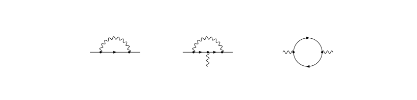
Figure 1: The elementary one-loop diagrams in QED

At one-loop level, only the following five elementary vertex functions are superficially UV divergent and hence have to be renormalized: the self-energy $\Sigma$, the electron-photon vertex $\Lambda_{\mu}$, the vacuum polarization $\Pi_{\mu\nu}$, the three- and four-point photon vertices. The Feynman diagrams for the first three vertices are given in Fig.1. The three-point photon vertex is zero due to Furry’s theorem, while, as will be shown below, the four point photon vertex is actually definite in our approach due to gauge invariance.

We first consider the vertex functions listed in Fig.1 whose Feynman integrals read,

$$-i\Sigma^{(1)}(p)\equiv(-ie)^{2}\int\frac{d^{4}l}{(2\pi)^{4}}\frac{i\left[(1-\xi)\frac{l^{\kappa}l^{\tau}}{l^{2}}-g^{\kappa\tau}\right]}{l^{2}+i\epsilon}\gamma_{\kappa}\frac{i}{/\!\!l+/\!\!\!p-m+i\epsilon}\gamma_{\tau};$$ (11)

$$\Lambda^{(1)}_{\mu}(p,\tilde{p})\equiv(-ie)^{2}\int\frac{d^{4}l}{(2\pi)^{4}}\frac{i\left[(1-\xi)\frac{l^{\kappa}l^{\tau}}{l^{2}}-g^{\kappa\tau}\right]}{l^{2}+i\epsilon}\gamma_{\kappa}\frac{i}{/\!\!l+/\!\!\!p-m+i\epsilon}$$

$$\quad\quad\quad\quad\quad\quad\times\gamma_{\mu}\frac{i}{/\!\!l+/\!\!\!\tilde{p}-m+i\epsilon}\gamma_{\tau};$$ (12)

$$i\Pi^{(1)}_{\mu\nu}(q)\equiv(-ie)^{2}\int\frac{d^{4}l}{(2\pi)^{4}}(-1)\texttt{Tr}\left[\gamma_{\mu}\frac{i}{/\!\!l-m+i\epsilon}\gamma_{\nu}\frac{i}{/\!\!l+/\!\!\!q-m+i\epsilon}\right],$$ (13)

where $p,\tilde{p}$ and $q$ denote the external momenta for electron and photon respectively. The superficial divergence degrees for the three diagrams are well-known: $\omega(\Sigma^{(1)})=1$, $\omega(\Lambda^{(1)}_{\mu})=0$, $\omega(\Pi^{(1)}_{\mu\nu})=2$. Note the routing of the external momenta are so chosen that they flow through the fermionic internal lines, which will yield convenience for calculations and a clear diagrammatic interpretation of the operation associated with the differentiation with respect to external momenta, see below. We will consider other routings for the self-energy and the vertex diagrams in the Appendix A.

III.1 Differential equations for divergent integrals

Below, we treat these superficially divergent integrals with the strategy described above, according to which the three differential equations are,

$$\partial_{p_{\alpha}}\partial_{p_{\beta}}\Sigma^{(1)}(p)=\Sigma^{(1);\alpha\beta}(p),$$ (14)

$$\partial_{p_{\alpha}}\Lambda^{(1)}_{\mu}(p,\tilde{p})=\Lambda^{(1);\alpha}_{\mu}(p,\tilde{p}),$$ (15)

$$\partial_{q_{\alpha}}\partial_{q_{\beta}}\partial_{q_{\gamma}}\Pi^{(1)}_{\mu\nu}(q)=\Pi^{(1);\alpha\beta\gamma}_{\mu\nu}(q),$$ (16)

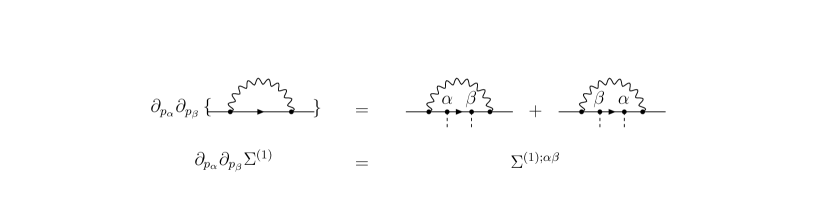
Figure 2: The graphical representation of Eq.(14).

where the right hand sides (RHS) of these differential equations are convergent Feynman diagrams, their corresponding loop integrals are listed in Appendix A. Actually, in terms of Feynman diagram the RHS of Eqs.(14,15,16) are just obtained through insertion of photon probes with zero momentum, provided that the external momentum flows through internal fermion lines, cf. Fig.2 for an example.

The loop integration on the RHS of Eqs.(14,15,16) can now be straightforwardly carried out:

$$-i\Sigma^{(1);\alpha\beta}(p)= \frac{8ie^{2}}{(4\pi)^{2}}\int^{1}_{0}\!\!\!z^{3}dz\left\{\frac{(z/\!\!\!p-2m)p^{\alpha}p^{\beta}}{z(zp^{2}-m^{2})^{2}}-\frac{g^{\alpha\beta}(/\!\!\!p-\frac{2m}{z})+\gamma^{\{\alpha}p^{\beta\}}}{2z(zp^{2}-m^{2})}\right.$$ (17)

$$\left.+(1-\xi)\left[\frac{(p^{2}-m^{2})/\!\!\!pp^{\alpha}p^{\beta}}{(zp^{2}-m^{2})^{3}}-\frac{(p^{2}-m^{2})(g^{\alpha\beta}/\!\!\!p+\gamma^{\{\alpha}p^{\beta\}})}{4z(zp^{2}-m^{2})^{2}}\right.\right.$$

$$\left.\left.-\frac{(6/\!\!\!p-2m)p^{\alpha}p^{\beta}}{4z(zp^{2}-m^{2})^{2}}+\frac{g^{\alpha\beta}(/\!\!\!p-\frac{m}{2})+\gamma^{\{\alpha}p^{\beta\}}}{2z^{2}(zp^{2}-m^{2})}\right]\right\},$$

$$\Lambda^{(1);\alpha}_{\mu}(p,\tilde{p})= -\frac{e^{2}}{(4\pi)^{2}}\int_{0}^{1}\!\!\!dy\int_{0}^{1-y}\!\!\!dz\left\{-\frac{4z\gamma_{\mu}(p-P)^{\alpha}}{\Delta}+\frac{2z(p-P)^{\alpha}\mathcal{G}_{\mu}}{\Delta^{2}}\right.$$ (18)

$$\left.+\gamma^{\sigma}\frac{(1-z)\gamma^{\alpha}\gamma_{\mu}(/\!\!\!\tilde{p}+m-/\!\!\!P)-z(/\!\!\!p+m-/\!\!\!P)\gamma_{\mu}\gamma^{\alpha}}{\Delta}\gamma_{\sigma}\right.$$

$$\left.+(1-\xi)(1-y-z)\left[\frac{4z(p-P)^{\alpha}\mathcal{F}_{1;\mu}}{\Delta^{3}}\right.\right.$$

$$\left.\left.+\frac{[z\gamma^{\alpha}(/\!\!\!p+m-/\!\!\!P)+(1-z)/\!\!\!P\gamma^{\alpha}]\gamma_{\mu}(/\!\!\!\tilde{p}+m-/\!\!\!P)/\!\!\!P}{\Delta^{2}}\right.\right.$$

$$\left.\left.+\frac{z/\!\!\!P(/\!\!\!p+m-/\!\!\!P)\gamma_{\mu}[(/\!\!\!\tilde{p}+m-/\!\!\!P)\gamma^{\alpha}-\gamma^{\alpha}/\!\!\!P]}{\Delta^{2}}\right.\right.$$

$$\left.\left.+\frac{2z(p-P)^{\alpha}\mathcal{F}_{2;\mu}}{\Delta^{2}}+\frac{3z\gamma_{\mu}/\!\!\!\tilde{p}\gamma^{\alpha}+3z\gamma^{\alpha}/\!\!\!p\gamma_{\mu}+3/\!\!\!P\gamma^{\alpha}\gamma_{\mu}}{\Delta}\right.\right.$$

$$\left.\left.+\frac{/\!\!\!\tilde{p}\gamma_{\mu}\gamma^{\alpha}+12z(p-2P)^{\alpha}\gamma_{\mu}+(6z-2)mg^{\alpha}_{\mu}}{\Delta}\right]\right\},$$

$$i\Pi^{(1);\alpha\beta\gamma}_{\mu\nu}(q)= \frac{2^{4}ie^{2}}{(4\pi)^{2}}\int^{1}_{0}\!\!\!z^{4}(1-z)^{4}dz\left\{\frac{g_{\mu}^{\{\alpha}q^{\beta}g^{\gamma\}}_{\nu}+q_{\{\mu}g_{\nu\}}^{\{\alpha}g^{\beta\gamma\}}-2g_{\mu\nu}g^{\{\alpha\beta}q^{\gamma\}}}{z^{2}(1-z)^{2}(m^{2}-z(1-z)q^{2})}\right.$$ (19)

$$\left.+\frac{q_{\{\mu}g_{\nu\}}^{\{\alpha}q^{\beta}q^{\gamma\}}-12g_{\mu\nu}q^{\alpha}q^{\beta}q^{\gamma}+(q_{\mu}q_{\nu}-p^{2}g_{\mu\nu})g^{\{\alpha\beta}q^{\gamma\}}}{z(1-z)(m^{2}-z(1-z)q^{2})^{2}}\right.$$

$$\left.+\frac{8(q_{\mu}q_{\nu}-q^{2}g_{\mu\nu})q^{\alpha}q^{\beta}q^{\gamma}}{(m^{2}-z(1-z)q^{2})^{3}}\right\},$$

$$P\equiv zp+y\tilde{p},\ \Delta\equiv(y+z)m^{2}+P^{2}-zp^{2}-y\tilde{p}^{2},$$

$$\mathcal{G}_{\mu}\equiv \gamma^{\sigma}(/\!\!\!p+m-/\!\!\!P)\gamma_{\mu}(/\!\!\!\tilde{p}+m-/\!\!\!P)\gamma_{\sigma},$$

$$\mathcal{F}_{1;\mu}\equiv /\!\!\!P(/\!\!\!p+m-/\!\!\!P)\gamma_{\mu}(/\!\!\!\tilde{p}+m-/\!\!\!P)/\!\!\!P,$$

$$\mathcal{F}_{2;\mu}\equiv /\!\!\!\tilde{p}\gamma_{\mu}/\!\!\!p+3\gamma_{\mu}/\!\!\!\tilde{p}/\!\!\!P+3/\!\!\!P/\!\!\!p\gamma_{\mu}+(m^{2}-6P^{2})\gamma_{\mu}+2m(3P_{\mu}-p_{\mu}-\tilde{p}_{\mu}).$$ (20)

Here symmetrization about Greek indices grouped in the bracket $\{\cdots\}$) is frequently used for brevity. The three definite functions then determine the original loop amplitudes up to certain degree of ambiguity. Next, we proceed to solving the differential equations using the above definite functions.

III.2 Solutions

Evidently, the direct integrating back with respect to external momenta would be cumbersome. Instead of doing so, we may first extract the differentiation with respect to external momenta in the following manner,

$$-i\Sigma^{(1);\alpha\beta}(p)= \partial_{p_{\alpha}}\partial_{p_{\beta}}\left\{\frac{ie^{2}}{(4\pi)^{2}}\int_{0}^{1}\!\!\!dz\left[[(1-2z-\xi)/\!\!\!p+(3+\xi)m]\ln(m^{2}-zp^{2})\right.\right.$$ (21)

$$\left.\left.-(1-\xi)\frac{z(p^{2}-m^{2})/\!\!\!p}{m^{2}-zp^{2}}\right]\right\},$$

$$\Lambda^{(1);\alpha}_{\mu}(p,\tilde{p})= \partial_{p_{\alpha}}\left\{-\frac{e^{2}}{(4\pi)^{2}}\int_{0}^{1}\!\!\!dy\int_{0}^{1-y}\!\!\!dz\left[2\gamma_{\mu}\ln\Delta+\frac{\mathcal{G}_{\mu}}{\Delta}+(1-\xi)(1-y-z)\right.\right.$$ (22)

$$\left.\left.\times\left(-6\gamma_{\mu}\ln\Delta+\frac{\mathcal{F}_{1;\mu}}{\Delta^{2}}+\frac{\mathcal{F}_{2;\mu}}{\Delta}\right)\right]\right\},$$

$$i\Pi^{(1);\alpha\beta\gamma}_{\mu\nu}(q)= \partial_{q_{\alpha}}\partial_{q_{\beta}}\partial_{q_{\gamma}}\left\{-\frac{8ie^{2}}{(4\pi)^{2}}(q_{\mu}q_{\nu}-g_{\mu\nu}q^{2})\int^{1}_{0}\!\!\!dzz(1-z)\right.$$ (23)

$$\left.\times\ln(m^{2}-z(1-z)q^{2})\right\},$$

then the solutions could be readily found as:

$$-i\Sigma^{(1)}(p) =\frac{ie^{2}}{(4\pi)^{2}}\left\{\int_{0}^{1}\!\!\!dz\left[[(1-2z-\xi)/\!\!\!p+(3+\xi)m]\ln(m^{2}-zp^{2})\right.\right.$$ (24)

$$\quad\left.\left.-\frac{(1-\xi)z(p^{2}-m^{2})/\!\!\!p}{m^{2}-zp^{2}}\right]+C_{\psi}/\!\!\!p+C_{m}\right\},$$

$$\Lambda^{(1)}_{\mu}(p,\tilde{p}) =-\frac{e^{2}}{(4\pi)^{2}}\left\{\int_{0}^{1}\!\!\!dy\int_{0}^{1-y\!\!\!}dz\left[2\gamma_{\mu}\ln\Delta+\frac{\mathcal{G}_{\mu}}{\Delta}+(1-\xi)(1-y-z)\right.\right.$$ (25)

$$\left.\left.\times\left(-6\gamma_{\mu}\ln\Delta+\frac{\mathcal{F}_{1;\mu}}{\Delta^{2}}+\frac{\mathcal{F}_{2;\mu}}{\Delta}\right)\right]+C_{\perp}\gamma_{\mu}\right\},$$

$$i\Pi^{(1)}_{\mu\nu}(q) =-\frac{8ie^{2}}{(4\pi)^{2}}\left[(q_{\mu}q_{\nu}-g_{\mu\nu}q^{2})\int^{1}_{0}\!\!\!dzz(1-z)\ln(m^{2}-z(1-z)q^{2})\right.$$ (26)

$$\quad\left.+C_{A}q_{\mu}q_{\nu}+\tilde{C}_{A}g_{\mu\nu}q^{2}+C_{\{\mu}q_{\nu\}}+C_{\mu\nu}+g_{\mu\nu}C_{\Pi;0}\right],$$

with $[C_{\cdots}]$ ($C_{\mu\nu}$ is traceless, $C^{\mu}_{\mu}=0$) being the corresponding integration constants that are ambiguous at present stage. They are uniquely defined only in the underlying formulation that is well defined at short distances, but in the effective theory, i.e., QED, they are free constants to be determined through appropriate boundary conditionsSter .

Actually, for photon vacuum polarization, Lorentz invariance could remove the constants $C_{\mu},C_{\mu\nu}$. The presence of $C_{\Pi;0}$ would violate gauge invariance, i.e, making the photon massive. To ensure gauge invariance, we must impose $C_{A}+\tilde{C}_{A}=C_{\Pi;0}=0$. For self-energy, both $C_{\psi}$ and $C_{m}$ preserve Lorentz invariance, but are gauge dependent. In our previous reports, the constants $[C_{\cdots}]$ are termed as ”agent” constants as they should be consequences of taking the ”decoupling” limit of $\{\sigma\}$. To further determine the residual constants, we must resort to more constraints from symmetries and finally from physical boundary conditions, which will be pursued in the following section. Before imposing boundary conditions, the net outcomes of conventional renormalization programs are also ambiguities, the true reflection of ill-definedness. The same is also true in EG approach. However, our strategy leads to the same outcome with neither complicated (also unnecessary) manipulation of infinities nor modification of Feynman rules at loop levels, hence, it is simple. So, the real problem is ambiguity (rather than divergence) to be fixed through appropriate boundary conditions.

Here, some more technical remarks are in order: (1) In the differential equation approach, any spurious violation of symmetries due to local ambiguities in the loop amplitudes could be easily removed. Therefore, the physical breakdown of symmetries (i.e., anomalies) must come from definite properties of the loop diagrams. Actually, it is shown in our previous studies that chiral and trace anomaliesanomaly1 ; anomaly2 ; anomaly3 ; trace1 ; trace2 ; trace3 ; trace4 ; trace5 ; trace6 do originate from the existence of definite or nonlocal terms like $(k_{\mu}k_{\nu}/{k^{2}})\check{\Gamma}$ in certain divergent integralsActa951 ; Acta952 ; thesis ; plb393 . After contraction with $k^{\mu}$ or $g^{\mu\nu}$, they give rise to local operators: (a) $k^{\mu}\cdot(k_{\mu}k_{\nu}/{k^{2}})\check{\Gamma}=k_{\nu}\check{\Gamma}$ (chiral anomaly)Acta951 ; Acta952 ; thesis , (b) $g^{\mu\nu}\cdot(k_{\mu}k_{\nu}/{k^{2}})\check{\Gamma}=\check{\Gamma}$ (trace anomaly)plb393 ; thesis . In contrast to spontaneous breaking of global symmetries where massless poles appear at tree level as consequences, certain massless poles show up in loop amplitudes as origins of the quantum mechanical violation of canonical symmetries. (2) Amusingly, this perspective of anomalies also imply that there may exist properties in divergent integrals that are both definite (nonlocal) and unexpected from canonical deductions. Therefore, such divergent diagrams contain more about quantum field theoriesthooft-diagram1 ; thooft-diagram2 . These properties might be viewed as indirect but definite links to underlying theory. (3) The differential equations used here also imply some structural relations between the Feynman diagrams. Actually, in QED, as there is no pure gauge boson loops, all the differentiations with respect to external momenta effectively amount to inserting the elementary QED vertex, or external photon with zero momentum. The final result amounts to the Ward identity in differential form. It will be interesting to see what will happen in more complicated theories with pure gauge boson loops, like non-Abelian theories. (4) Technically, one could not obtain a polynomial/local term from convolution of non-polynomial/nonlocal functions. A mathematically natural way to yield a polynomial/local term is to perform certain limit operation. To our interest, this mathematical scenario corroborates the underlying theory scenario: The computation should be followed by the ”low-energy” limit due to the wide separation of scales, then some local terms arise from the ”low-energy” limit, indicating the existence of underlying structures. Conventionally, a regularization is introduced as a rough substitute of the underlying structures and is taken to zero in the final stage after removing the ”dusts” (infinities) brought about by the regularization. In our strategy, we simply appreciate the existence of the underlying structures and then solve the differential equations that must be satisfied by the limiting objects.

III.3 Comparing with Dimensional Regularization

Now we list out the results from dimensional scheme for a comparison. Our conclusion is that at one-loop level the only difference between the two approaches lies in the local part, which is in fact prescription dependent. The definite (nonlocal) part must be prescription independent and hence physical. The two approaches are equivalent if one takes the local part in dimensional scheme as ambiguous. From this equivalence one could devise a simple method for computation: do the calculations in dimensional regularization, then replace the local part with ambiguous polynomials of the corresponding degree. However, this equivalence is only valid after sub-divergences are subtracted in case of multi-loop diagrams ctp38 .

The results from dimensional scheme read,

$$-i\Sigma^{(1)}(p;\epsilon)= \frac{ie^{2}}{(4\pi)^{2}}\left\{\int_{0}^{1}\!\!\!dz\left[[(1-2z-\xi)/\!\!\!p+(3+\xi)m]\ln\frac{m^{2}-zp^{2}}{4\pi\mu^{2}}\right.\right.$$ (27)

$$\left.\left.-\frac{(1-\xi)z(p^{2}-m^{2})/\!\!\!p}{m^{2}-zp^{2}}\right]+\left(\epsilon^{-1}-\gamma_{E}+\frac{1}{2}\right)(/\!\!\!p-4m)\right.$$

$$\left.-(1-\xi)\left(\epsilon^{-1}-\gamma_{E}+1\right)(/\!\!\!p-m)\right\}+o(\epsilon),$$

$$\Lambda^{(1)}_{\mu}(p,\tilde{p};\epsilon)= -\frac{e^{2}}{(4\pi)^{2}}\left\{\int_{0}^{1}\!\!\!dy\int_{0}^{1-y}\!\!\!dz\left[2\gamma_{\mu}\ln\Delta+\frac{\mathcal{G}_{\mu}}{\Delta}+(1-\xi)(1-y-z)\right.\right.$$ (28)

$$\left.\left.\times\left(-6\gamma_{\mu}\ln\Delta+\frac{\mathcal{F}_{1;\mu}}{\Delta^{2}}+\frac{\mathcal{F}_{2;\mu}}{\Delta}\right)\right]\right.-\epsilon^{-1}+\gamma_{E}+2$$

$$\left.+(1-\xi)\left(\epsilon^{-1}-\gamma_{E}-\frac{5}{6}\right)\gamma_{\mu}\right\}+o(\epsilon),$$

$$i\Pi^{(1)}_{\mu\nu}(q;\epsilon)= -\frac{8ie^{2}}{(4\pi)^{2}}\left[(q_{\mu}q_{\nu}-g_{\mu\nu}q^{2})\int^{1}_{0}\!\!\!dzz(1-z)\ln\frac{m^{2}-z(1-z)q^{2}}{4\pi\mu^{2}}\right]$$ (29)

$$+\frac{4ie^{2}}{3(4\pi)^{2}}\left(\epsilon^{-1}-\gamma_{E}\right)(q_{\mu}q_{\nu}-g_{\mu\nu}q^{2})+o(\epsilon).$$

We note that in terms of the above parametrization, the following correspondence between the agent constants and the local constants in dimensional regularization could be easily established:

$$\ C_{\psi}\leftrightarrow C_{\psi}(\epsilon)\equiv\xi\left(\epsilon^{-1}-\gamma_{E}+1+\ln\left(4\pi\mu^{2}\right)\right)-\frac{1}{2},$$

$$\frac{C_{m}}{m}\leftrightarrow\frac{C_{m}(\epsilon)}{m}\equiv-(3+\xi)\left(\epsilon^{-1}-\gamma_{E}+\ln\left(4\pi\mu^{2}\right)\right)-1-\xi,$$

$$\ C_{\perp}\leftrightarrow C_{\perp}(\epsilon)\equiv-\xi\left(\epsilon^{-1}-\gamma_{E}-\frac{5}{6}+\ln\left(4\pi\mu^{2}\right)\right)+\frac{7}{6},$$

$$\ C_{A}\leftrightarrow C_{A}(\epsilon)\equiv-\frac{1}{6}\left(\epsilon^{-1}-\gamma_{E}+\ln\left(4\pi\mu^{2}\right)\right).$$ (30)

Obviously, the dimensional regularized results exactly agree with ours obtained from Eqs.(14,15,16) after replacing the divergent constants by the agent constants following the correspondence (III.3). In other words, the dimensional regularization results (after or before subtraction) could be seen as a particular solution to our differential equations at one-loop level. At multi-loop level, the dimensional results will also satisfy such differential equations loop by loop after all the corresponding sub-divergences are removedctp38 .

III.4 Reducing ambiguities with Ward identities

Since gauge invariance is encoded in the Ward identities among various vertices, it is natural to ask if these identities are satisfied for the loop amplitudes computed in our approach. Specifically, we wish to examine the status of the following Ward identity for self-energy and vertex function,

$$\partial_{p^{\mu}}\Sigma^{(1)}(p)=-\Lambda^{(1)}_{\mu}(p,p),$$ (31)

in our approach.

To proceed, we make use of the results in dimensional regularization and look at the Feynman gauge components, i.e., those remain when $\xi=1$, the rest components will be delegated to Appendix B. Carrying out the parametric integrations, we have,

$$-i\Sigma^{(1)}(p;\epsilon) =\frac{ie^{2}}{(4\pi)^{2}}\left\{\left[\epsilon^{-1}-\gamma_{E}+1-\ln\frac{m^{2}}{4\pi\mu^{2}}+\delta+(\delta^{2}-1)\ln\frac{\delta-1}{\delta}\right]/\!\!\!p\right.$$ (32)

$$\quad\left.-\left[\epsilon^{-1}-\gamma_{E}+\frac{3}{2}-\ln\frac{m^{2}}{4\pi\mu^{2}}+(\delta-1)\ln\frac{\delta-1}{\delta}\right]4m\right\}$$

$$=\frac{ie^{2}}{(4\pi)^{2}}\left\{\left[C_{\psi}(\epsilon)\|_{\xi=1}+\frac{1}{2}-\ln m^{2}+\delta+(\delta^{2}-1)\ln\frac{\delta-1}{\delta}\right]/\!\!\!p\right.$$

$$\quad\left.-\left[\frac{C_{m}(\epsilon)}{4m}\|_{\xi=1}+1-\ln m^{2}+(\delta-1)\ln\frac{\delta-1}{\delta}\right]4m\right\},$$

$$\Lambda^{(1)}_{\mu}(p,p;\epsilon) =\frac{e^{2}}{(4\pi)^{2}}\left\{\left[\epsilon^{-1}-\gamma_{E}+1-\ln\frac{m^{2}}{4\pi\mu^{2}}+\delta+(\delta^{2}-1)\ln\frac{\delta-1}{\delta}\right]\gamma_{\mu}\right.$$ (33)

$$\quad\left.-2\left[2\left(\delta\ln\frac{\delta-1}{\delta}+1\right)(\delta/\!\!\!p-2m)+/\!\!\!p\right]\frac{p_{\mu}}{p^{2}}\right\}$$

$$=\frac{e^{2}}{(4\pi)^{2}}\left\{\left[-C_{\perp}(\epsilon)\|_{\xi=1}+3-\ln m^{2}+\delta+(\delta^{2}-1)\ln\frac{\delta-1}{\delta}\right]\gamma_{\mu}\right.$$

$$\quad\left.-2\left[2\left(\delta\ln\frac{\delta-1}{\delta}+1\right)(\delta/\!\!\!p-2m)+/\!\!\!p\right]\frac{p_{\mu}}{p^{2}}\right\},$$

with $\delta\equiv\frac{m^{2}}{p^{2}}$. The constants $C_{\psi}(\epsilon),C_{\perp}(\epsilon)$ have been defined in the correspondence (III.3). Now differentiating $\Sigma^{(1)}(p;\epsilon)$ with respect to $p^{\mu}$, it is trivial to verify the Ward identity (31) in dimensional regularization:

$$-i\partial_{p^{\mu}}\Sigma^{(1)}(p;\epsilon) =\frac{ie^{2}}{(4\pi)^{2}}\left\{\left[\epsilon^{-1}-\gamma_{E}+1-\ln\frac{m^{2}}{4\pi\mu^{2}}+\delta+(\delta^{2}-1)\ln\frac{\delta-1}{\delta}\right]\gamma_{\mu}\right.$$ (34)

$$\quad\left.-2\left[2\left(\delta\ln\frac{\delta-1}{\delta}+1\right)(\delta/\!\!\!p-2m)+/\!\!\!p\right]\frac{p_{\mu}}{p^{2}}\right\}$$

$$=i\Lambda^{(1)}_{\mu}(p,p;\epsilon).$$

It is easy to see that in dimensional regularization this Ward identity is ensured by the following relation,

$$C_{\psi}(\epsilon)\|_{\xi=1}+C_{\perp}(\epsilon)\|_{\xi=1}=\frac{5}{2}.$$

In general gauge, we have (Cf. Appendix B):

$$C_{\psi}(\epsilon)+C_{\perp}(\epsilon)=\frac{4+11\xi}{6}.$$ (35)

Evidently, replacing $C_{\psi}(\epsilon),C_{\perp}(\epsilon)$ with $C_{\psi},C_{\perp}$, one enters our approach. Thus the Ward identity (31) could hold in our approach only when the agent constants $C_{\psi}$ and $C_{\perp}$ satisfy the same relation as that between $C_{\psi}(\epsilon)$ and $C_{\perp}(\epsilon)$:

$$C_{\psi}+C_{\perp}=\frac{4+11\xi}{6}.$$ (36)

That means, gauge invariance constrains the agent constants $C_{\psi}$ and $C_{\perp}$ according to Eq.(36). Obviously, such constraints are just welcome in our approach to reduce the ambiguities. Of course, at higher orders, such constraints must be also consistently imposed. At one-loop level, there is in principle no obstacle to remove the local violations of any symmetries. As removal of the local ambiguities never affects the nonlocal and hence definite part, any physical anomaly must be originated from definite and hence prescription-independent sources. As mentioned above, at least for chiral and trace anomalies, this is indeed the case: a type of mass-independent and definite terms is the true source of quantum mechanical violations of the canonical chiral and scale transformationsActa951 ; Acta952 ; thesis ; plb393 .

Therefore, due to Lorentz and gauge invariance, we are left with three ambiguous constants to fix: $C_{\psi}$, $C_{m}$ and $C_{A}$. This statement is, however, a little bit cursory before the finiteness of the rest superficially divergent diagrams, i.e., the three- and four-photon vertex functions, is established. Below we turn to these diagrams. Since the three-photon vertex does not contribute to cross sections or physical observables according to Furry’s theorem, we only need to verify the finiteness of the four-photon vertex, that is, there is no ultraviolet ambiguity in this vertex function which is again ensured by gauge invariance.

III.5 Finiteness of the four-photon vertex

To verify that the four-photon vertex is free of ambiguity, it suffices to show that the most divergent piece in each individual diagram cancel out against each other due to gauge invariance.

The external momenta and polarizations of the four external photon are arranged in the following manner: $(p_{1},\mu),(p_{2},\nu),(p_{3},\rho),(p_{4},\sigma)$ with $p_{4}=-p_{1}-p_{2}-p_{3}$ due to conservation of the four dimensional momentum, i.e., $p_{1}$ always enters at vertex $\mu$, $p_{2}$ at $\nu$, etc. The four-photon vertex consists of six inequivalent individual Feynman diagrams that differ from each other by the arrangement of the relative positions of the external photons along the internal fermion loop. It is convenient to fix the position of the first photon of $(p_{1},\mu)$ and let the other photons move to obtain the rest inequivalent loop diagrams. The notations for the four-photon vertex and the six individual diagrams are as follows,

$$\Gamma_{\mu\nu\rho\sigma}(p_{1},p_{2},p_{3},p_{4}) = \Gamma_{1;\mu\nu\rho\sigma}(p_{1},p_{2},p_{3},p_{4})+\Gamma_{2;\mu\rho\nu\sigma}(p_{1},p_{3},p_{2},p_{4})$$ (37)

$$+\Gamma_{3;\mu\nu\sigma\rho}(p_{1},p_{2},p_{4},p_{3})+\Gamma_{4;\mu\sigma\rho\nu}(p_{1},p_{4},p_{3},p_{2})$$

$$+\Gamma_{5;\mu\sigma\nu\rho}(p_{1},p_{4},p_{2},p_{3})+\Gamma_{6;\mu\rho\sigma\nu}(p_{1},p_{3},p_{4},p_{2}).$$

The Feynman integral for $\Gamma_{1;\mu\nu\rho\sigma}$ reads,

$$i\Gamma_{1;\mu\nu\rho\sigma}= (-ie)^{4}\int\frac{-d^{4}l}{(2\pi)^{4}}\texttt{Tr}\left(\frac{i}{/\!\!l-m+i\epsilon}\gamma_{\mu}\frac{i}{/\!\!l+/\!\!\!p_{1}-m+i\epsilon}\gamma_{\nu}\right.$$ (38)

$$\times\left.\frac{i}{/\!\!l+/\!\!\!p_{1}+/\!\!\!p_{2}-m+i\epsilon}\gamma_{\rho}\frac{i}{/\!\!l+/\!\!\!p_{1}+/\!\!\!p_{2}+/\!\!\!p_{3}-m+i\epsilon}\gamma_{\sigma}\right).$$

By rearranging the external momenta and the elementary vertices, one could readily obtain the integrals for the rest five diagrams. Since the superficial divergence degree of such diagrams is 0, then it suffices to verify that the logarithmic divergence is absent in the sum of the six diagrams in order that gauge invariance is preserved. Obviously, it suffices to do computation with $\Gamma_{1;\mu\nu\rho\sigma}$ as others could be obtained by permutations of the vertices $(p_{1},\mu),(p_{2},\nu),\cdots$.

Differentiating the integral in Eq.(38) with respect to $p_{1;\alpha}$, the resulting integral becomes definite and gives,

$$\partial_{p_{1;\alpha}}i\Gamma_{1;\mu\nu\rho\sigma} =\frac{8ie^{4}}{(4\pi)^{2}}T_{1;\mu\nu\rho\sigma}\int_{0}^{1}\!\!\!dx\int_{0}^{x}\!\!\!dy\int_{0}^{y}\!\!\!dz\partial_{p_{1;\alpha}}\ln\tilde{\Delta}_{1}+\partial_{p_{1;\alpha}}i\check{\Gamma}_{1;\mu\nu\rho\sigma},$$ (39)

$$T_{1;\mu\nu\rho\sigma} \equiv g_{\mu\nu}g_{\rho\sigma}-2g_{\mu\rho}g_{\nu\sigma}+g_{\mu\sigma}g_{\nu\rho},$$ (40)

$$\tilde{\Delta}_{1} \equiv m^{2}-(x-x^{2})p_{1}^{2}-(y-y^{2})p_{2}^{2}-(z-z^{2})p_{3}^{2}$$ (41)

$$\quad-2y(1-x)p_{1}p_{2}-2z(1-x)p_{1}p_{3}-2z(1-y)p_{2}p_{3},$$

where the $\check{\Gamma}_{1;\mu\nu\rho\sigma}$ denotes the definite parts after integrating back with respect to $p_{1;\alpha}$ and is not concerned here. Next, integrating back with respect to $p_{1;\alpha}$, the diagram $\Gamma_{1;\mu\nu\rho\sigma}$ could be parametrized as follows:

$$i\Gamma_{1;\mu\nu\rho\sigma}=\frac{8ie^{4}}{(4\pi)^{2}}T_{1;\mu\nu\rho\sigma}\int_{0}^{1}\!\!\!dx\int_{0}^{x}\!\!\!dy\int_{0}^{y}\!\!\!dz\ln\frac{\tilde{\Delta}_{1}}{C_{1;4\gamma}}+\check{\Gamma}_{1;\mu\nu\rho\sigma},$$ (42)

where an integration constant $C_{1;4\gamma}$ is shown explicitly, which is exactly the ambiguity that corresponds to the logarithmic divergence of the integral in Eq.(38). The results for other diagrams are given in Appendix C. For later convenience, we integrate by parts with respect to the Feynman parametric integration to arrive at the following expressions for $\Gamma_{1;\mu\nu\rho\sigma}$,

$$i\Gamma_{1;\mu\nu\rho\sigma}=\frac{4ie^{4}}{3(4\pi)^{2}}T_{1;\mu\nu\rho\sigma}\ln\frac{m^{2}}{C_{1;4\gamma}}+\tilde{\Gamma}_{1;\mu\nu\rho\sigma},$$ (43)

where the definite terms arising from this operation have been absorbed into $\check{\Gamma}_{1;\mu\nu\rho\sigma}$ and collectively denoted as $\tilde{\Gamma}_{1;\mu\nu\rho\sigma}$, cf. Appendix D.

Now, in order that the ill-defined piece in the full amplitude vanish

$$i\Gamma_{\mu\nu\rho\sigma}\|_{\texttt{ill-defined}} =\frac{4ie^{4}}{3(4\pi)^{2}}\left[\sum_{k=1}^{6}T_{k;\mu\nu\rho\sigma}\ln\frac{m^{2}}{C_{k;4\gamma}}\right]=0,$$ (44)

with $\sum_{k=1}^{6}T_{k;\mu\nu\rho\sigma}=0$, the constant $C_{k;4\gamma}$ must be identical for each $k$ (say, $C_{k;4\gamma}=\bar{C}_{4\gamma},\forall k$). Otherwise, gauge invariance will be violated. Thus, similar as the case of vacuum polarization for two-photon vertex, gauge invariance also remove the ambiguities in the four-photon vertex function.

In fact, after setting all the external momenta to zero, we will end up with the same ill-defined integral in all the six diagrams:

$$\int\frac{d^{4}l}{(2\pi)^{4}}\frac{l_{a}l_{b}l_{c}l_{d}}{(l^{2}-m^{2})^{4}}=-\frac{i}{24(4\pi)^{2}}[g_{ab}g_{cd}+\cdots]\ln\frac{m^{2}}{\bar{C}_{4\gamma}}.$$ (45)

Thus it is natural to deem that the constants $C_{k;4\gamma}$ are identical in any reasonable prescription.

In dimensional regularization, one would find the following correspondence in each of the six diagrams:

$$\ln\frac{m^{2}}{C_{k;4\gamma}}\leftrightarrow-\epsilon^{-1}+\gamma_{E}+\ln\frac{m^{2}}{{4\pi\mu^{2}}},$$

which means the full four-photon vertex is finite in dimensional regularization due to the mechanism demonstrated above.

III.6 Brief summary of differential equation approach to QED at one-loop level

Now, we have treated all the superficially divergent or ill-defined loop diagrams of QED at one-loop level, without resorting to any artificial deformation of spacetime and symmetries or any form of cutoffs. At one-loop level, only three local ambiguities remain to be fixed in QED: $C_{\psi}$, $C_{m}$ and $C_{A}$ that appear in self-energy $\Sigma$, vertex $\Lambda_{\mu}$ and vacuum polarization $\Pi_{\mu\nu}$, respectively. This is a natural conclusion following from Lorentz and gauge invariance and the existence of a complete underlying theory.

In particular, from our treatment, one could naturally infer that, any fundamental theory that is well defined and underlies the presently known QED must also yield the same or equivalent functional expressions as given here after taking the ”decoupling” limit, the only difference is that the unknown agent constants could be unambiguously computed in such underlying theory. Therefore, in the underlying theory perspective, the QED processes defined by the elementary Feynman diagrams (in covariant gauge) represented by Fig.1 must take the following form,

$$-i\Sigma^{(1)}(p)= \frac{ie^{2}}{(4\pi)^{2}}\left\{\int_{0}^{1}\!\!\!dz\left[[(1-2z-\xi)/\!\!\!p+(3+\xi)m]\ln\frac{m^{2}-zp^{2}}{\mu^{2}_{\text{UD}}}\right.\right.$$ (46)

$$\left.\left.-\frac{(1-\xi)z(p^{2}-m^{2})/\!\!\!p}{m^{2}-zp^{2}}\right]+c^{0}_{\psi}/\!\!\!p+c^{0}_{m}m\right\},$$

$$\Lambda^{(1)}_{\mu}(p,\tilde{p})= -\frac{e^{2}}{(4\pi)^{2}}\left\{\int_{0}^{1}\!\!\!dy\int_{0}^{1-y}\!\!\!dz\left[2\gamma_{\mu}\ln\Delta+\frac{\mathcal{G}_{\mu}}{\Delta}+(1-\xi)(1-y-z)\right.\right.$$ (47)

$$\left.\left.\times\left(-6\gamma_{\mu}\ln\Delta+\frac{\mathcal{F}_{1;\mu}}{\Delta^{2}}+\frac{\mathcal{F}_{2;\mu}}{\Delta}\right)\right]+\left(\frac{4+11\xi}{6}-c^{0}_{\psi}\right)\gamma_{\mu}\right\},$$

$$i\Pi^{(1)}_{\mu\nu}(q)= \frac{8ie^{2}(g_{\mu\nu}q^{2}-q_{\mu}q_{\nu})}{(4\pi)^{2}}\left[\int^{1}_{0}\!\!\!dzz(1-z)\ln\frac{m^{2}-z(1-z)q^{2}}{\mu^{2}_{\text{UD}}}+c^{0}_{A}\right],$$

where we have explicitly ”separated out” a dimensional constant $\mu_{\text{UD}}$ from all the constants $C_{\cdots}$ to balance the dimension in the logarithmic parts, the residual parts are purely dimensionless numbers, each denoted as $c^{0}_{\cdots}$. This way of parametrizing the constants will be more precise and useful for the following discussions.

We should also note that, in the underlying theory perspective, all the constants or parameters that appear in the Lagrangian should be defined from the ”decoupling” limit of the underlying theory also as ”agents”. In our view, these ”agents” in lagrangian are only elementary from the perspective of (effective) field theories, not necessary so in the perspective of underlying theory. As the agent constants appear in the local part of the elementary vertex functions within perturbative framework, the Lagrangian constants would mix with these local terms containing the agent constants in the corresponding vertex functions. This is in fact the origin of renormalization group equations in our approach, without resorting to the conventional renormalization theory, see, Sec. IV for a brief discussion.

IV Removing ambiguities and ”renormalization” scheme

Now we turn to determining the ambiguous agent constants. Obviously, the conventional renormalization schemes would be reproduced provided that the ambiguous constants as well as mass and couplings are fixed through the conventional renormalization conditions. An appropriate choice of the whole set $\{m,e;\mu,c^{0}_{\cdots}\}$ defines a renormalization prescription or scheme. So, our simple strategy is compatible with the conventional renormalization programs. In principle, any scheme can be employed provided the same scattering matrix elements or the same physical observables could be obtained. This freedom just leads to the renormalization group in the general sense of Stückelberg-PetermanSP . Fixing the dimensionless constants in a scheme and letting the scale $\mu_{\text{UD}}$ vary, one could obtain the renormalization group equations in the narrow sense.

To proceed, the following parametrization would be used useful,

$$\Sigma^{(1)}(p) =A^{(1)}(p^{2})/\!\!\!p+B^{(1)}(p^{2})m,$$ (49)

$$\bar{u}(p)\Lambda^{(1)}_{\mu}u(\tilde{p}) =\bar{u}(p)\gamma_{\mu}u(\tilde{p})F^{(1)}(k^{2})+\frac{i\bar{u}(p)\sigma_{\mu\nu}k^{\nu}u(\tilde{p})}{2m}G^{(1)}(k^{2}),$$ (50)

$$\Pi^{(1)}_{\mu\nu}(q) =-\Pi^{(1)}(q^{2})(g_{\mu\nu}q^{2}-q_{\mu}q_{\nu}),$$ (51)

$$A^{(1)}(p^{2}) \equiv-\frac{\alpha}{4\pi}\left[\xi\left(\left(\delta^{2}-1\right)\ln\frac{\delta-1}{\delta}+\delta-\ln\frac{m^{2}}{\mu^{2}_{\text{UD}}}\right)+\frac{1}{2}+c^{0}_{\psi}\right],$$ (52)

$$B^{(1)}(p^{2}) \equiv\frac{\alpha}{4\pi}\left[(3+\xi)\left((\delta-1)\ln\frac{\delta-1}{\delta}+1-\ln\frac{m^{2}}{\mu^{2}_{\text{UD}}}\right)-c^{0}_{m}\right],$$ (53)

$$F^{(1)}(k^{2}) \equiv\frac{\alpha}{4\pi}\left[2\text{arccoth}[\theta_{k}]\left[\left(1+\ln\frac{\lambda_{\gamma}}{m^{2}}\right)\left(\theta_{k}+\frac{1}{\theta_{k}}\right)+\theta_{k}\right]+2\right.$$ (54)

$$\left.\quad-{\Xi}(k^{2};1-\xi)-\ln\frac{m^{2}}{\mu^{2}_{\text{UD}}}-c^{0}_{\perp}\right],$$

$$G^{(1)}(k^{2}) \equiv\frac{\alpha}{2\pi}\left(\theta_{k}-\frac{1}{\theta_{k}}\right)\text{arccoth}[\theta_{k}],$$ (55)

$$\Pi^{(1)}(q^{2}) \equiv\frac{\alpha}{3\pi}\left[\theta_{q}\left(\theta_{q}^{2}-3\right)\text{arccoth}[\theta_{q}]-\theta_{q}^{2}-\ln\frac{m^{2}}{\mu^{2}_{\text{UD}}}+\frac{8}{3}-6c^{0}_{A}\right],$$ (56)

$$\delta =\frac{m^{2}}{p^{2}},\ k=p-\tilde{p},\ \theta_{x}\equiv\sqrt{1-\frac{4m^{2}}{x^{2}}}.$$ (57)

Note that the vertex function is sandwiched between on-shell states $[u(\tilde{p}),\bar{u}(p)]$ of electron. Obviously, the scalar factors $A^{(1)},B^{(1)},F^{(1)}$ and $\Pi^{(1)}$ contain ultra-violet ambiguities (depending on $c^{0}_{\psi},c^{0}_{m},c^{0}_{\perp}$ and $c^{0}_{A}$, respectively). Moreover, the first three factors are also gauge dependent and infrared singular when the external momenta are on mass shell. In $F^{(1)}$, we have explicitly put in a photon mass squared ($\lambda_{\gamma}$) to regulate the infrared singularity, with ${\Xi}$ denoting the terms proportional to $1-\xi$. In contrast, the scalar factor $G^{(1)}$ is both ultra-violet and infrared finite and also gauge independent. Its value at zero momentum transfer ($k^{2}=0$) gives the well-known anomalous magnetic moment of electron at one-loop level:

$$G^{(1)}(0)=\frac{\alpha}{2\pi}.$$

IV.1 Various boundary conditions for vertex function

Now we impose various conditions on the elementary vertices (here, $\Sigma^{(1)},\Lambda^{(10}_{\mu},\Pi^{(1)}_{\mu\nu}$). In doing so, both the tree level parameters ($m,e$) and the agent constants must be understood as scheme-dependent so that the observables computed using these parameters and vertices are physical and independent of schemes. The lagrangian or tree level mass or coupling needs not be just the physical one, which may differ by a ”(re)normalization” constant in the conventional terminology. In our strategy, such ”(re)normalization” constants could also be introduced but are nevertheless ultra-violet finite. Actually, as is already pointed out in Ref.weinbergvol1 : ”the renormalization of mass and field has nothing directly to do with the presence of infinities, and would be necessary even in a theory in which all momentum space integrals are convergent”.

IV.1.1 On-shell conditions

First, let us consider the so-called on-shell conditions in Feynman gauge, which read,

$$\Sigma^{(1)}\|_{/\!\!\!p=m}=0,\ \partial_{/\!\!\!p}\Sigma^{(1)}\|_{/\!\!\!p=m}=0,\ \Lambda^{(1)}_{\mu}\|_{/\!\!\!p=/\!\!\!\tilde{p}=m}=0,\ \Pi^{(1)}\|_{q^{2}=0}=0.$$ (58)

Using the expressions given above, we could find that:

$$\Sigma^{(1)}\|_{/\!\!\!p=m} =\frac{\alpha}{4\pi}\left(-3\ln\frac{m^{2}}{\mu^{2}_{\text{UD}}}+\frac{5}{2}-c^{0}_{\psi}-c^{0}_{m}\right)m,$$

$$\partial_{/\!\!\!p}\Sigma^{(1)}\|_{/\!\!\!p=m} =\frac{\alpha}{4\pi}\left(\ln\frac{m^{2}}{\mu^{2}_{\text{UD}}}-2\ln\frac{\lambda_{\gamma}}{m^{2}}-\frac{7}{2}-c^{0}_{\psi}\right),$$

$$\Lambda^{(1)}_{\mu}\|_{/\!\!\!p=/\!\!\!\tilde{p}=m} =\frac{\alpha}{4\pi}\left(-\ln\frac{m^{2}}{\mu^{2}_{\text{UD}}}+2\ln\frac{\lambda_{\gamma}}{m^{2}}+\frac{7}{2}+c^{0}_{\psi}\right)\gamma_{\mu},$$

$$\Pi^{(1)}\|_{q^{2}=0} =\frac{\alpha}{3\pi}\left(-\ln\frac{m^{2}}{\mu^{2}_{\text{UD}}}-6c^{0}_{A}\right),$$ (59)

where $c^{0}_{\psi}+c^{0}_{\perp}=5/2$ has been used. Note that all the infrared singularities have been regularized with a photon mass, and $m$ now denotes the physical mass for electron. According to conventional programs, the coupling $e$ or $\alpha=e^{2}/(4\pi)$ appearing in these conditions is understood to be the physical one.

Then the on-shell conditions could be fulfilled provided the constants $[c^{0}_{\cdots}]$ take the following values:

$$c^{0}_{\psi}=\ln\frac{m^{2}}{\mu^{2}_{\text{UD}}}-2\ln\frac{\lambda_{\gamma}}{m^{2}}-\frac{7}{2}=\frac{5}{2}-c^{0}_{\perp},$$

$$c^{0}_{m}=-4\ln\frac{m^{2}}{\mu^{2}_{\text{UD}}}+2\ln\frac{\lambda_{\gamma}}{m^{2}}+6,\quad c^{0}_{A}=-\frac{1}{6}\ln\frac{m^{2}}{\mu^{2}_{\text{UD}}}.$$ (60)

In this manner, all the ambiguities are gone in the vertices, including the scale $\mu_{\text{UD}}$:

$$A^{(1)}_{os}(p^{2}) \equiv-\frac{\alpha}{4\pi}\left[\left(\delta^{2}-1\right)\ln\frac{\delta-1}{\delta}+\delta-3-2\ln\frac{\lambda_{\gamma}}{m^{2}}\right],$$ (61)

$$B^{(1)}_{os}(p^{2}) \equiv\frac{\alpha}{4\pi}\left[4(\delta-1)\ln\frac{\delta-1}{\delta}-2-2\ln\frac{\lambda_{\gamma}}{m^{2}}\right],$$ (62)

$$F^{(1)}_{os}(k^{2}) \equiv\frac{\alpha}{4\pi}\left[2\text{arccoth}[\theta_{k}]\left[\left(1+\ln\frac{\lambda_{\gamma}}{m^{2}}\right)\left(\theta_{k}+\frac{1}{\theta_{k}}\right)+\theta_{k}\right]\right.$$ (63)

$$\quad\left.-4-2\ln\frac{\lambda_{\gamma}}{m^{2}}\right]$$

$$\Pi^{(1)}_{os}(q^{2}) \equiv\frac{\alpha}{3\pi}\left[\theta_{q}\left(\theta_{q}^{2}-3\right)\text{arccoth}[\theta_{q}]-\theta_{q}^{2}+\frac{8}{3}\right].$$ (64)

The on-shell scheme works for field theories without unstable fields as elementary quantum degrees of freedom. The tree level mass is identified as the physical pole mass. But for complicated theories like electroweak with unstable sectors, the on-shell scheme runs into trouble, see Ref.unstable1 ; unstable2 ; unstable3 ; unstable4 ; unstable5 ; unstable6 ; unstable7 ; unstable8 ; unstable9 ; unstable10 .

IV.1.2 ”Minimal” conditions

In analogy to the famous ”Minimal Subtraction”, one may define a scheme where $[c^{0}_{\cdots}]$ are removed so that only the $\sim\ln\mu^{2}$ pieces are left over, which will lead to the well-known mass-independent running behavior. We will denote this scheme as ”Ms”, which may also be interpreted as ”Minimal specification”.

Since $c^{0}_{\psi}$ and $c^{0}_{\perp}$ can not be zero at the same time due to gauge invariance, we choose the following:

$$c^{0}_{\psi}+\frac{1}{2}=c^{0}_{m}=c^{0}_{A}=0,\quad c^{0}_{\perp}=3.$$ (65)

Then the prescription-dependent scalar factors would take the following neater forms (in Feynman gauge):

$$A^{(1)}_{Ms}(p^{2}) \equiv-\frac{\alpha}{4\pi}\left[\left(\delta^{2}-1\right)\ln\frac{\delta-1}{\delta}+\delta-\ln\frac{m^{2}}{\mu^{2}_{Ms}}\right],$$ (66)

$$B^{(1)}_{Ms}(p^{2}) \equiv\frac{\alpha}{\pi}\left[(\delta-1)\ln\frac{\delta-1}{\delta}+1-\ln\frac{m^{2}}{\mu^{2}_{Ms}}\right],$$ (67)

$$F^{(1)}_{Ms}(k^{2}) \equiv\frac{\alpha}{4\pi}\left[2\text{arccoth}[\theta_{k}]\left[\left(1+\ln\frac{\lambda_{\gamma}}{m^{2}}\right)\left(\theta_{k}+\frac{1}{\theta_{k}}\right)+\theta_{k}\right]\right.$$ (68)

$$\quad\left.-1-\ln\frac{m^{2}}{\mu^{2}_{Ms}}\right],$$

$$\Pi^{(1)}_{Ms}(q^{2}) \equiv\frac{\alpha}{3\pi}\left[\theta_{q}\left(\theta_{q}^{2}-3\right)\text{arccoth}[\theta_{q}]-\theta_{q}^{2}+\frac{8}{3}-\ln\frac{m^{2}}{\mu^{2}_{Ms}}\right].$$ (69)

Here the subscript ”$Ms$” for mass $m$ and coupling $e$ are omitted to avoid heavy symbolism and the scale $\mu_{\text{UD}}$ is now replaced by $\mu_{Ms}$. Of course, the concrete values for $m$ and $e$ in this scheme need to be determined in terms of physical values of mass using appropriate physical observablesSter . In this prescription, the scalar factors $A$ and $B$ at general off-shell momenta are not beset with infrared singularities in contrast to the on-shell prescription.

IV.1.3 Boundary conditions at vanishing off-shell momenta

One could also impose boundary conditions at off-shell momenta. Among these off-shell prescriptions, the zero momenta case is much simpler for QED with massive fermion. In Feynman gauge, we have:

$$\Sigma^{(1)}\|_{/\!\!\!p=0} =\frac{\alpha}{4\pi}\left(-4\ln\frac{m^{2}}{\mu^{2}_{\text{UD}}}-c^{0}_{m}\right)m,$$

$$\partial_{/\!\!\!p}\Sigma^{(1)}\|_{/\!\!\!p=0} =\frac{\alpha}{4\pi}\left(\ln\frac{m^{2}}{\mu^{2}_{\text{UD}}}-c^{0}_{\psi}\right),$$

$$\Lambda^{(1)}_{\mu}\|_{/\!\!\!p=/\!\!\!\tilde{p}=0} =\frac{\alpha}{4\pi}\left(-\ln\frac{m^{2}}{\mu^{2}_{\text{UD}}}+\frac{5}{2}-c^{0}_{\perp}\right)\gamma_{\mu},$$

$$\Pi^{(1)}\|_{q=0} =\frac{\alpha}{3\pi}\left(-\ln\frac{m^{2}}{\mu^{2}_{\text{UD}}}-6c^{0}_{A}\right),$$ (70)

so they vanish if

$$c^{0}_{\psi}=\ln\frac{m^{2}}{\mu^{2}_{\text{UD}}}=\frac{5}{2}-c^{0}_{\perp},\ c^{0}_{m}=-4\ln\frac{m^{2}}{\mu^{2}_{\text{UD}}},\ c^{0}_{A}=-\frac{1}{6}\ln\frac{m^{2}}{\mu^{2}_{\text{UD}}}.$$ (71)

Then the scalar factors read:

$$A^{(1)}_{zm}(p^{2}) \equiv-\frac{\alpha}{4\pi}\left[\left(\delta^{2}-1\right)\ln\frac{\delta-1}{\delta}+\delta+\frac{1}{2}\right],$$ (72)

$$B^{(1)}_{zm}(p^{2}) \equiv\frac{\alpha}{\pi}\left[(\delta-1)\ln\frac{\delta-1}{\delta}+1\right],$$ (73)

$$F^{(1)}_{zm}(k^{2}) \equiv\frac{\alpha}{4\pi}\left[2\text{arccoth}[\theta_{k}]\left[\left(1+\ln\frac{\lambda_{\gamma}}{m^{2}}\right)\left(\theta_{k}+\frac{1}{\theta_{k}}\right)+\theta_{k}\right]-\frac{1}{2}\right],$$ (74)

$$\Pi^{(1)}_{zm}(q^{2}) \equiv\frac{\alpha}{3\pi}\left[\theta_{q}\left(\theta_{q}^{2}-3\right)\text{arccoth}[\theta_{q}]-\theta_{q}^{2}+\frac{8}{3}\right].$$ (75)

The nice point of off-shell conditions at zero momenta (hence the subscript ”$zm$”) is that, the infrared singularities do not show up in the scalar factors at general off-shell momenta, just like in the ”$Ms$” prescription. Such conditions possess an intuitive interpretation: at zero momenta, quantum fluctuations are suppressed, and an electron would serve as a classical static source of electromagnetic field, with the tree level coupling ”$e$” being pertinent to static or Coulomb charge somehow.

IV.1.4 Physical boundary conditions in terms of observables

In principle, boundary conditions may be imposed upon many other field-theoretical objects that are constructed with elementary vertex functions or Green function. It would be better to work with the observables that could be readily confronted with physical data and depend on the elementary parameters (masses, couplings, and agent constants) in an as simple as possible manner, sparing the intermediate renormalization.

For example, one may proceed as below in QED: First, physical values are assigned to the Lagrangian parameters (masses and couplings), the agent constants are treated as unknown or arbitrary; Second, appropriate observables are selected that could be readily expressed in terms of Feynman diagrams that definitely contain the agent constants; Finally, the agent constants could be fixed in terms of the physical parameters and data of these observables. In formulae,

$$(1) \quad\{m,e;[C_{\cdots}]\}\Rightarrow\{m^{\text{(phy)}},e^{(\text{phy})};[C^{(\text{phy})}_{\cdots}]\},$$

$$(2) \quad Q_{n}\left(m^{(\text{phy})},e^{(\text{phy})};[C^{(\text{phy})}_{\cdots}]\right)=Q^{\texttt{(data)}}_{n},\ n=1,2,\cdots$$ (76)

$$\Rightarrow C^{(\text{phy})}_{\cdots}=f_{\cdots}\left([Q^{\texttt{(data)}}_{n}];m^{(\text{phy})},e^{(\text{phy})}\right).$$

The set of observables to be employed for this purpose should fulfill some natural requirements such as simplicity and analyticity with respect to their dependence upon mass, coupling and the agent constants, well-definedness in the infrared, etc. In principle, even theories like quantum chromodynamics (QCD) that are elusive of physical pole masses of elementary quantum fields can be treated in this manner, where the physical contents of the lagrangian or tree level masses and couplings becomes a nontrivial issue. Such imposition of physical boundary conditions is general and natural from underlying theory perspective. Actually, this is exactly what is done in literature for the determination of the ”physical” coupling of strong interaction, see, e.g., Ref.Ster , chapter 12.

IV.1.5 A remark on boundary conditions

In order that the same observables are obtained, different choices of ”intermediate” boundary conditions or prescriptions for vertex functions must be related to each other somehow, or more specifically, the transformations across different prescriptions defined by the boundary conditions should in principle be feasible, at least within perturbation theory. In conventional programs, this is the so-called scheme dependence in perturbation theory, where different renormalization conditions or prescriptions, differ by a set of finite renormalization constants, and the observables computed in different prescriptions should agree with each other to the perturbation order computed. This is in fact encoded in the renormalization group equation in the sense of Stückelberg-Peterman as mentioned in the very beginning of this section. Furthermore, a general prescription would also contain an arbitrary scale as ”renormalization point”. The variation of this arbitrary scale within the specified prescription should not affect observables, which would in effect lead to renormalization group equations that are themselves prescription- or scheme-dependent.

The above statements make perfect sense within perturbative framework. However, things might become complicated in nonperturbative contexts. As an simple example, we refer to our previous workPRD65 , where it is shown that some scheme in incompatible with dynamical symmetry breaking of massless $\lambda\phi^{4}$ theory in nonperturbative context. Strictly speaking, any intermediate boundary conditions or prescriptions to be employed must be in the same ”orbit” as the physical boundaries. This in turn requires a complete solution of the full theory of quantum fields, which is presently out of our reach. So, scheme dependence is a real issue for quantum field theories beyond perturbative regime.

IV.1.6 Influences of infrared divergences

It is well-known that QED is beset with infrared divergences. For on-shell scheme, infrared divergences show up already in the boundary conditions for the loop amplitudes, as is evident above. Simply speaking, infrared singularity arises because Fock states could not work well in presence of massless particles. Thus introducing certain extent of coherence, the infrared divergences in QED could be removed by use of Bloch-Nordsieck theoremBN , which has been described in detail in many standard field theory textbooks, e.g., Ster ; peskin ; weinbergvol1 . At one loop level, one regularize the infrared singularities in the loop diagrams somehow (here in this report, in terms of a fictitious photon mass) and they will cancel out against those from real diagrams in physical observables.

Of course, for more complicated non-Abelian gauge theories, severe infrared divergences are present and their treatments are more involved. Nevertheless, as our approach do not alter anything in the infrared, so all the conventional methods for dealing with infrared singularities or similar singularities except the ultraviolet ones may well apply. As is clear from our above discussions, one may work with a set of renormalization conditions that are not plagued by infrared singularities to avoid further complications, this could be done with conditions or ”boundaries” defined at off-shell momenta where everything is infrared finiteKPQ1 ; KPQ2 , e.g., at zero four-momenta as illustrated above.

IV.2 Lagrangian perspective

In this subsection, we reexamine the issue in terms of lagrangian or action, which allows us to examine a number of issues in a more transparent manner. Such effort is also helpful to resolve some conceptual difficulties that have been ”afflicting” the conventional practices.

IV.2.1 Brief review of conventional programs

The conventional program of renormalization starts with a bare lagrangian:

$$\mathcal{L}(\psi_{B},A_{B}^{\mu};m_{B},e_{B})={\bar{\psi}}_{B}(i/\!\!\!\!D_{B}-m_{B})\psi_{B}-\frac{1}{4}F_{B;\mu\nu}F_{B}^{\mu\nu}-\frac{1}{2\xi_{B}}(\partial_{\mu}A_{B}^{\mu})^{2},$$ (77)

with $D^{\mu}_{B}=\partial^{\mu}-ie_{B}A_{B}^{\mu}$. Then all the 1PI vertices $\left(\Gamma^{n}_{B}([p_{1},\cdots,p_{n}],m_{B},e_{B})\right)$ are renormalized through the following renormalization rescaling,

$$\psi_{B}=Z_{\psi}^{1/2}\psi,\ A_{B}^{\mu}=Z_{A}^{1/2}A^{\mu},\ m_{B}=\frac{Z_{m}}{Z_{\psi}}m,\ e_{B}=(Z_{A})^{-1/2}e,\ \xi_{B}=Z_{A}\xi,$$ (78)

and

$$\mathcal{L}(\psi_{B},A_{B}^{\mu};m_{B},e_{B}) =Z_{\psi}{\bar{\psi}}i/\!\!\!\!D\psi-Z_{m}m{\bar{\psi}}\psi-\frac{Z_{A}}{4}F_{\mu\nu}F^{\mu\nu}-\frac{1}{2\xi}(\partial_{\mu}A^{\mu})^{2}$$ (79)

$$=\mathcal{L}(\psi,A^{\mu};m,e)+\Delta\mathcal{L}(\psi,A^{\mu};Z_{\psi}-1,Z_{m}-1,Z_{A}-1),$$

so that

$$\Gamma^{(n)}_{B}([p_{1},\cdots,p_{n}],m_{B},e_{B})=Z^{-n_{\psi}/2}_{\psi}Z^{-n_{A}/2}_{A}\Gamma^{(n)}([p_{1},\cdots,p_{n}],m,e).$$ (80)

Here, $\Delta\mathcal{L}$ serves to provide all the necessary counter-terms for canceling out any divergences in the loop diagrams. As the BPHZ algorithm is equivalent to the above program, below, we will refer to both as conventional approaches or programs. One caveat is that the formalism for such programs is only established within the realm of perturbation and hence must be so implemented.

IV.2.2 Underlying theory perspective

Now, let us reexamine the same issue from underlying theory perspective. It is convenient to work with the path integral formulation. In terms of a underlying theory description, the generating functional for the QED processes would formally take the following form:

$$Z(J_{\mu},\eta,\bar{\eta};\{\sigma\})= \int\!\!d\mu[\phi_{\text{UT}}]\exp\left\{i\int\!\!d^{4}x\left[\mathcal{L}_{\text{UT}}([\phi_{\text{UT}}],\{\sigma\})\right.\right.$$ (81)

$$\left.\left.+J_{\mu}O^{\mu}_{A}(\{\sigma\})+O_{\bar{\psi}}(\{\sigma\})\eta+\bar{\eta}O_{\psi}(\{\sigma\})\right]\right\},$$

where $[\phi_{\text{UT}}]$ is used to label all the necessary degrees of freedom, and $O^{\mu}_{A},O_{\bar{\psi}},O_{\psi}$ denotes the photon and electron field parameters in the UT description which may well be composite ones.

At ”lower” scales where QED become prominent or effective processes, all the typical higher energy modes are actually integrated out, resulting in a well-defined functional in terms of dominant or effective degrees,

$$Z(J_{\mu},\eta,\bar{\eta};\{\sigma\})= \int\!\!dA^{\mu}d\bar{\psi}d\psi\exp\left\{i\int\!\!d^{4}x\left[\mathcal{L}_{\text{eff}}(\psi,A_{\mu};\{\sigma\})\right.\right.$$ (82)

$$\left.\left.+J_{\mu}A^{\mu}+\bar{\psi}\eta+\bar{\eta}\psi\right]\right\},$$

with $\int\!d^{4}x\mathcal{L_{\text{eff}}}(\psi,A_{\mu};\{\sigma\})$ being the effective action generated from the integrating-out. Taking the ”decoupling limit” ($\breve{\mathcal{P}}_{\texttt{\scriptsize LE}}$) naïvely on the effective lagrangian would yield to a classical lagrangian of QED,

$$\breve{\mathcal{P}}_{\texttt{\scriptsize LE}}[\mathcal{L}_{\text{eff}}(\psi,A_{\mu};\{\sigma\})]=\mathcal{L}_{\text{QED}}(\psi,A_{\mu}),$$ (83)

which in turn leads to ill-defined path integral as the limit operation and the functional integration does not commute. Obviously, the details taken away with the limit operation,

$$\delta\mathcal{L}(\psi,A_{\mu};\{\sigma\})\equiv \mathcal{L}_{\text{eff}}(\psi,A_{\mu};\{\sigma\})-\breve{\mathcal{P}}_{\texttt{\scriptsize LE}}[\mathcal{L}_{\text{eff}}(\psi,A_{\mu};\{\sigma\})]$$

$$= \mathcal{L}_{\text{eff}}(\psi,A_{\mu};\{\sigma\})-\mathcal{L}_{\text{QED}}(\psi,A_{\mu}),$$

is just what we are missing for a well defined path integral. Therefore, we must include it into the path integral,

$$Z(J_{\mu},\eta,\bar{\eta};\{\sigma\})= \int\!\!dA^{\mu}d\bar{\psi}d\psi\exp\left\{i\int\!\!d^{4}x\left[\mathcal{L}_{\text{QED}}(\psi,A_{\mu})+\delta\mathcal{L}(\psi,A_{\mu};\{\sigma\})\right.\right.$$ (84)

$$\left.\left.+J_{\mu}A^{\mu}+\bar{\psi}\eta+\bar{\eta}\psi\right]\right\}.$$

Evidently, in conventional programs, $\delta\mathcal{L}$ is implemented through regularization and subtraction that are encoded in $\Delta\mathcal{L}$. For certain interactions, the job of $\Delta\mathcal{L}$ could be ”autonomously” done using operators appearing in the classical lagrangian, leading in effect to the ”renormalization” of these operators. Such autonomous cases are conventionally termed as renormalizable, while the rest as un-renormalizable. As a ”realization” or substitute of $\delta\mathcal{L}$, $\Delta\mathcal{L}$ must also take the responsibility to clear all the side effects like ultraviolet infinities associated with a regularization. Only in this sense, the manipulation of infinities (through counter terms) may be justifiable, and the bare lagrangian may serve as a symbolic and rough representation of the underlying theory: $\mathcal{L}_{\text{eff}}(\psi,A_{\mu};\{\sigma\})$, which definitely contains the sophisticated underlying quantum details that could not be simply described in terms of ”bare” objects that are originally coined in classical field theory.

As we could at best obtain the parametric form of the ”decoupling” effects of $\{\sigma\}$, there may be certain arbitrariness in our choice of $\mathcal{L}_{\text{QED}}=\breve{\mathcal{P}}_{\texttt{\scriptsize LE}}[\mathcal{L}_{\text{eff}}]$ (that is actually unknown to us yet) as our ”starting” lagrangian for calculations or the in the separation of it out of $\mathcal{L}_{\text{eff}}$:

$$\mathcal{L}_{\text{eff}}=\tilde{\mathcal{L}}_{\text{QED}}+\tilde{\delta}\mathcal{L}(\cdots;\{\sigma\})=\mathcal{L}_{\text{QED}}+\delta\mathcal{L}(\cdots;\{\sigma\}),$$

where $\tilde{\mathcal{L}}_{\text{QED}}$ and $\mathcal{L}_{\text{QED}}$ would at most differ by a series of local operators (for renormalizable theories, by a finite ”renormalization” of the lagrangian) that could be absorbed into $\delta\mathcal{L}(\cdots;\{\sigma\})$:

$$\delta\mathcal{L}(\cdots;\{\sigma\})=\delta_{\text{var}}\mathcal{L}_{\text{QED}}+\tilde{\delta}\mathcal{L}(\cdots;\{\sigma\}),\quad\delta_{\text{var}}\mathcal{L}_{\text{QED}}\equiv\tilde{\mathcal{L}}_{\text{QED}}-\mathcal{L}_{\text{QED}}.$$

Obviously, any sensible prescription of $\breve{\mathcal{P}}_{\texttt{\scriptsize LE}}[\mathcal{L}_{\text{eff}}]$ should necessarily include a reference scale that are widely separated from the underlying ones. This natural appearance of a reference scale just corresponds to and hence remove the mystery around the dimensional transmutation phenomenon in the conventional programs.

IV.3 Origin of renormalization group equations

We note that renormalization group (RG) and RG equations (RGE) appear in terms of intermediate renormalization reparametrization, for which a lucid discussion can be found in Ref.muta . If we could proceed with all parameters being physical, there seems to be no room for it. However, as discussed above, even starting with a physical parametrization, one could still arrive at an arbitrary prescription, provided the prescription is related to the physical one via proper transformations. In this short subsection, we will not repeat the derivation of RGE in a specific scheme defined by the corresponding boundary conditions as is done in conventional programs, instead, we briefly show that the RGE like equations could be generically derived as a ”decoupling” theorem in terms of underlying structures even if the parameters are determined by physical boundary conditionsPLB6251 ; PLB6252 ; PLB6253 .

First let us look at the scaling law of QED in terms of underlying theory. For any 1PI $n$-point vertex function $\Gamma^{(n)}$, the scaling law would read,

$$\Gamma^{(n)}([\lambda p],[\lambda m,e];\{\lambda^{d_{\sigma}}\sigma\})=\lambda^{d_{\Gamma^{(n)}}}\Gamma^{(n)}([p],[m,e];\{\sigma\}),$$ (85)

with $d_{\cdots}$ denoting the canonical scaling dimension (equals to the mass dimension) of the corresponding parameter. The differential form of this scaling law reads,

$$\left\{\sum_{p}p\cdot\partial_{p}+m\partial_{m}+\sum_{\sigma}d_{\sigma}\sigma\partial_{\sigma}-d_{\Gamma^{(n)}}\right\}\Gamma^{(n)}([p],[m,e];\{\sigma\})=0.$$ (86)

Now applying the ”decoupling” limit to this differential equation, we have,

$$\left\{\sum_{p}p\cdot\partial_{p}+m\partial_{m}+\sum_{i}d_{C_{i}}C_{i}\partial_{C_{i}}-d_{\Gamma^{(n)}}\right\}\Gamma^{(n)}([p],[m,e];[C_{i}])=0,$$ (87)

with

$$\sum_{i}d_{C_{i}}C_{i}\partial_{C_{i}}\Gamma^{(n)}=\breve{\mathcal{P}}_{\texttt{\scriptsize LE}}\left(\sum_{\sigma}d_{\sigma}\sigma\partial_{\sigma}\Gamma^{(n)}\right)$$ (88)

denoting the contributions arising from the ”decoupling” limit operation.

Note that, in whatever prescription for the agent constants $[C_{i}]$, the scaling of these constants would just elicit insertion of appropriate local operators with respect to each loop where agent constants show up:

$$\sum_{i}d_{C_{i}}C_{i}\partial_{C_{i}}\Gamma^{(n)}=\sum_{a}\delta_{O_{a}}\check{I}_{O_{a}}\Gamma^{(n)},$$ (89)

where $\check{I}_{O_{a}}$ denotes the insertion of a local operator $O_{a}$ that corresponds to a vertex whose 1PI loop corrections contain local ambiguities with $\delta_{O_{a}}$ being the associated coefficients. At least at one-loop level in QED, only logarithmic ambiguities will be really contributing to these ”decoupling” effects that are anomalous in terms of the canonical contents of quantum field theories. Thus, $\delta_{O_{a}}$ is the primitive ”anomalous dimension” of operator $O_{a}$. A closer analysis will tell that among the operators $[O_{a}]$, there must be kinetic ones for which the above variations would induce an extra finite ”renormalization” of certain field operators, the rest must be characterizing interactions for which the variations would give rise to beta functions of their couplingsPLB6251 ; PLB6252 ; PLB6253 . So, Eq.(89) is our primitive form of renormalization group equations for a general prescription, which could be naturally interpreted as a ”decoupling theorem” of the underlying structures that regulate the ultra-violet regions of our quantum field theories. Obviously, imposing different boundary conditions would lead to different form of $\sum_{i}d_{C_{i}}C_{i}\partial_{C_{i}}$ and $\sum_{a}\delta_{O_{a}}\check{I}_{O_{a}}$.

In fact, one could recast the scaling law of Eq.(87) into the following concise form

$$\{p\cdot\partial_{p}-d_{\Gamma^{(n)}}\}\Gamma^{(n)}([p],[m,e];[C_{i}]) ={\hat{I}}_{i\tilde{\Theta}}\Gamma^{(n)}([p],[m,e];[C_{i}])$$ (90)

$$=\Gamma^{(n)}_{i\tilde{\Theta}}([0;p],[m,e];[C_{i}]),$$

with ${\hat{I}}_{i\tilde{\Theta}}\equiv-m\partial_{m}-\sum_{i}d_{C_{i}}C_{i}\partial_{C_{i}}$ denoting the insertion of the full trace of the stress tensor $\tilde{\Theta}^{\mu\nu}$ that contains trace anomalies due to renormalization. This equation is just an alternative form of the Callan-Symanzik equation, from which some low-energy theorems of QCD follow as immediate corollariesJPA40 .

V Discussions and summary

Before closing our presentation, we wish to make the following remarks about our simple strategy for renormalization: (1) As we introduce no artificial deformation of all the canonical structures or symmetries, hence not affecting spacetime dimension and Dirac algebra, thus our strategy could be applied to any field theory, such as supersymmetric and chiral field theories. (2) Since our ignorance about the underlying theory is parametrized in a general manner, the effects of regularization upon field theory and corresponding physics could be examined in a general manner. In particular, the physical origin of field theoretical properties like anomalies could be unambiguously identified and disentangled with the regularization effects in this strategy, surpassing the traditional interpretations that rely on effects of regularization. (3) Various operations such as external momenta routing and shift of loop variables are allowed in our simple strategy, sparing many subtleties associated these operations in the conventional approaches. Hence, one could better focus on more physical issues in calculations or identify true physical origins of various phenomena within field theoretical contexts. (4) In theoretical perspective, our approach is also useful in exploring whether or to what extent the underlying structures are compatible with the canonical symmetries or properties of quantum field theories, such as Lorentz invariance, various gauge symmetries, unitarity and so on. From a more practical viewpoint, our approach or similar strategies allows us to examine how our ignorance about underlying structures could be safely treated with the helps of these canonical symmetries. Obviously, more works need to be done both in the construction and applications of efficient programs using the simple strategy and in the exploration of various issues that are intricate with respect to the issue of regularization and renormalization.

In summary, we demonstrated in details with QED at one-loop level how a simple strategy for renormalization could work without introducing any specific form of regularization and manipulations of ultra-violet infinities. Some technical operations like loop variable shifting or momenta routing that are subtle issues in conventional programs are shown to be of no problem. In this simple strategy, ambiguities arise instead of infinities, which could be further reduced by imposing appropriate Ward identities. For the Lorentz and gauge invariant QED at one-loop level, it is shown in a prescription-independent manner that there are only three ambiguities to be fixed using appropriate boundary conditions. The conventional renormalization programs were also analyzed from the underlying theory perspective with the rationale of manipulation of ultra-violet infinities being explicated. Finally, the renormalization-group-like equations arise generically as ”decoupling theorems” of the underlying structures.

Appendix A

In this appendix, we list the convergent integrals that appear in the RHS of Eqs.(14,15,16),

$$-i\Sigma^{(1);\alpha\beta}(p)= (-ie)^{2}\int\frac{d^{4}l}{(2\pi)^{4}}\frac{i\left[(1-\xi)\frac{l^{\kappa}l^{\tau}}{l^{2}}-g^{\kappa\tau}\right]}{l^{2}+i\epsilon}\gamma_{\kappa}\frac{i}{/\!\!l+/\!\!\!p-m+i\epsilon}$$ (91)

$$\times\left[\gamma^{\alpha}\frac{-1}{/\!\!l+/\!\!\!p-m+i\epsilon}\gamma^{\beta}+(\alpha\leftrightarrow\beta)\right]\frac{-1}{/\!\!l+/\!\!\!p-m+i\epsilon}\gamma_{\tau};$$

$$\Lambda_{\mu}^{(1);\alpha}(p,\tilde{p})= (-ie)^{2}\int\frac{d^{4}l}{(2\pi)^{4}}\frac{i\left[(1-\xi)\frac{l^{\kappa}l^{\tau}}{l^{2}}-g^{\kappa\tau}\right]}{l^{2}+i\epsilon}\gamma_{\kappa}\frac{i}{/\!\!l+/\!\!\!p-m+i\epsilon}\gamma^{\alpha}$$ (92)

$$\times\frac{-1}{/\!\!l+/\!\!\!p-m+i\epsilon}\gamma_{\mu}\frac{i}{/\!\!l+/\!\!\!\tilde{p}-m+i\epsilon}\gamma_{\tau};$$

$$i\Pi^{(1);\alpha\beta\gamma}_{\mu\nu}(q)= (-ie)^{2}\int\frac{(-)d^{4}l}{(2\pi)^{4}}\texttt{Tr}\left[\gamma_{\mu}\frac{i}{/\!\!l-m+i\epsilon}\gamma_{\nu}\frac{i}{/\!\!l+/\!\!\!q-m+i\epsilon}\gamma^{\alpha}\right.$$ (93)

$$\times\left.\frac{-1}{/\!\!l+/\!\!\!q-m+i\epsilon}\gamma^{\beta}\frac{-1}{/\!\!l+/\!\!\!q-m+i\epsilon}\gamma^{\gamma}\frac{-1}{/\!\!l+/\!\!\!q-m+i\epsilon}\right]$$

$$+\texttt{permutations of}(\alpha,\beta,\gamma).$$

Obviously, these diagrams result in from zero momentum insertion of photon lines into the original diagrams that are ill-defined, Cf. Fig. 2 for a diagrammatic representation for the case of self-energy diagram.

As stated in Sec. II and III, other choices of routing only lead to equivalent results. For the self-energy diagram, we could let the external momentum $p$ of fermion flow through the photon line, so that the RHS of Eq.(14) reads,

$$-i\Sigma^{(1);\text{alt}}(p)=(-ie)^{2}\int\!\!\frac{d^{4}l}{(2\pi)^{4}}\frac{i\left[(1-\xi)\frac{(l-p)^{\kappa}(l-p)^{\tau}}{(l-p)^{2}}-g^{\kappa\tau}\right]}{(l-p)^{2}+i\epsilon}\gamma_{\kappa}\frac{i}{/\!\!l-m+i\epsilon}\gamma_{\tau}.$$

It is nothing else but the original one with the loop momentum shifted by $p$. Then applying our method to this integration, we arrived the following,

$$-i\Sigma^{(1);\text{alt}}(p)= \frac{ie^{2}}{(4\pi)^{2}}\left\{\int_{0}^{1}\!\!dz\left[[(z(2-3z)+z(3z-4)\xi)/\!\!\!p+(4+2z(\xi-1))m]\right.\right.$$

$$\left.\left.\times\ln(m^{2}-zp^{2})-(1-\xi)z(1-z)\frac{p^{2}(m+z/\!\!\!p)}{m^{2}-zp^{2}}\right]+\tilde{C}_{\psi}/\!\!\!p+\tilde{C}_{m}\right\},$$

which is equivalent to the form of the self-energy diagram as given in Eq.(24) after carrying out the parametric integrations, and the constants may differ from the those in Eq.(24) by a finite amount. Indeed, computing the difference between this routing and that given in Eq.(24), we have,

$$-i(\Sigma^{(1);\text{alt}}-\Sigma^{(1)})=\frac{ie^{2}}{(4\pi)^{2}}\left\{\left(\tilde{C}_{\psi}-C_{\psi}+\frac{(\xi-1)}{2}\right)/\!\!\!p+\tilde{C}_{m}-C_{m}\right\}.$$ (96)

Thus the two routings produce identical result after setting

$$\tilde{C}_{\psi}=C_{\psi}+\frac{(1-\xi)}{2},\quad\tilde{C}_{m}=C_{m},$$ (97)

which is natural from the underlying theory perspective where we should have $-i(\Sigma^{(1);\text{alt}}-\Sigma^{(1)})=0$. Of course, one could also verify this point using a consistent regularization method like dimensional scheme. This is an illustration of the theorem of routing in case (a) given in Sec. II.

Alternatively, we could proceed as follows: First, we could find the following from what we obtained above

$$-i\Sigma^{(1)}\|_{p=0}= \frac{ie^{2}}{(4\pi)^{2}}\left[C_{m}+(3+\xi)m\ln m^{2}\right],$$ (98)

$$-i\Sigma^{(1);\text{alt}}\|_{p=0}= \frac{ie^{2}}{(4\pi)^{2}}\left[\tilde{C}_{m}+(3+\xi)m\ln m^{2}\right].$$ (99)

Next note that,

$$-i\Sigma^{(1)}\|_{p=0}= (-ie)^{2}\int\frac{d^{4}l}{(2\pi)^{4}}\frac{i\left[(1-\xi)\frac{l^{\kappa}l^{\tau}}{l^{2}}-g^{\kappa\tau}\right]}{l^{2}+i\epsilon}\gamma_{\kappa}\frac{i}{/\!\!l-m+i\epsilon}\gamma_{\tau}$$

$$= -i\Sigma^{(1);\text{alt}}\|_{p=0},$$ (100)

which implies $C_{m}=\tilde{C}_{m}$. In the same fashion, we could find that

$$-i\partial_{p^{\alpha}}\Sigma^{(1)}\|_{p=0}= \frac{ie^{2}}{(4\pi)^{2}}\left[C_{\psi}-\xi\ln m^{2}+\frac{1-\xi}{2}\right]\gamma_{\alpha},$$ (101)

$$-i\partial_{p^{\alpha}}\Sigma^{(1);\text{alt}}\|_{p=0}= \frac{ie^{2}}{(4\pi)^{2}}\left[\tilde{C}_{\psi}-\xi\ln m^{2}\right]\gamma_{\alpha}.$$ (102)

Then from underlying theory perspective the two quantities $-i\partial_{p^{\alpha}}\Sigma^{(1)}\|_{p=0}$ and $-i\partial_{p^{\alpha}}\Sigma^{(1);\text{alt}}\|_{p=0}$ should be identical and hence $\tilde{C}_{\psi}=C_{\psi}+\frac{(1-\xi)}{2}$. In fact, the integral forms of these two quantities look different from each other, but it could be verified in any consistent regularization (e.g., dimensional regularization) that their difference is zero,

$$-i\partial_{p^{\alpha}}(\Sigma^{(1)}-\Sigma^{(1);\text{alt}})\|_{p=0} =\int\frac{d^{4}l}{(2\pi)^{4}}\frac{e^{2}(3-\xi)\gamma^{\beta}}{l^{2}(l^{2}-m^{2})}\left[g_{\beta\alpha}-\frac{2l_{\beta}l_{\alpha}}{l^{2}}-\frac{2l_{\beta}l_{\alpha}}{l^{2}-m^{2}}\right]$$ (103)

$$=0,$$

therefore they are identical in any consistent regularization scheme (including the postulated underlying theory), and the case (a) of the theorem of routing in Sec. II is verified.

We also note that the routing for the vertex diagram given above are so chosen that the calculations are less laborious, i.e., the two external fermion lines carry independent momenta so that the differentiation with respect to $p$ only operates on one internal line. One could well try the following more conventional routing,

$$\Lambda_{\mu}^{(1);\alpha}(p,p+q)= (-ie)^{2}\int\frac{d^{4}l}{(2\pi)^{4}}\frac{i\left[(1-\xi)\frac{l^{\kappa}l^{\tau}}{l^{2}}-g^{\kappa\tau}\right]}{l^{2}+i\epsilon}\gamma_{\kappa}\frac{i}{/\!\!l+/\!\!\!p-m+i\epsilon}$$ (104)

$$\times\left[\gamma^{\alpha}\frac{-1}{/\!\!l+/\!\!\!p-m+i\epsilon}\gamma_{\mu}+\gamma_{\mu}\frac{-1}{/\!\!l+/\!\!\!p+/\!\!\!q-m+i\epsilon}\gamma^{\alpha}\right]$$

$$\times\frac{i}{/\!\!l+/\!\!\!p+/\!\!\!q-m+i\epsilon}\gamma_{\tau}.$$

The final results for $\Lambda_{\mu}$ should be the same after we set $q=\tilde{p}-p$ in the solutions. After quite some algebras, we found that the vertex computed using this routing reads,

$$\Lambda^{(1);\alpha}_{\mu}(p,p+q)= \partial_{p_{\alpha}}\left\{-\frac{e^{2}}{(4\pi)^{2}}\int_{0}^{1}\!\!\!dy\int_{0}^{1-y}\!\!\!dz\left[2\gamma_{\mu}\ln\tilde{\Delta}+\frac{\tilde{\mathcal{G}}_{\mu}}{\tilde{\Delta}}+(1-\xi)(1-y-z)\right.\right.$$

$$\left.\left.\times\left(-6\gamma_{\mu}\ln\tilde{\Delta}+\frac{\tilde{\mathcal{F}}_{1;\mu}}{\tilde{\Delta}^{2}}+\frac{\tilde{\mathcal{F}}_{2;\mu}}{\tilde{\Delta}}\right)\right]\right\},$$

$$\tilde{P}\equiv (y+z)p+yq,\ \tilde{\Delta}\equiv(y+z)m^{2}+\tilde{P}^{2}-zp^{2}-y(p+q)^{2},$$

$$\tilde{\mathcal{G}}_{\mu}\equiv \gamma^{\sigma}(/\!\!\!p+m-/\!\!\!\tilde{P})\gamma_{\mu}(/\!\!\!p+/\!\!\!q+m-/\!\!\!\tilde{P})\gamma_{\sigma},$$

$$\tilde{\mathcal{F}}_{1;\mu}\equiv /\!\!\!\tilde{P}(/\!\!\!p+m-/\!\!\!\tilde{P})\gamma_{\mu}(/\!\!\!p+/\!\!\!q+m-/\!\!\!\tilde{P})/\!\!\!\tilde{P},$$

$$\tilde{\mathcal{F}}_{2;\mu}\equiv (/\!\!\!p+/\!\!\!q)\gamma_{\mu}/\!\!\!p+3\gamma_{\mu}(/\!\!\!p+/\!\!\!q)/\!\!\!\tilde{P}+3/\!\!\!\tilde{P}/\!\!\!p\gamma_{\mu}+(m^{2}-6\tilde{P}^{2})\gamma_{\mu}$$ (105)

$$+2m(3\tilde{P}_{\mu}-2p_{\mu}-q_{\mu}).$$

It is immediate to see that this result exactly agrees with that given above after setting $\tilde{p}=p+q$, as asserted by the theorem of routing in case (b) presented in Sec. II.

Appendix B

Here, we consider the Ward identity for the components proportional to $1-\xi$ that are listed as below:

$$-i\frac{\Delta\Sigma^{(1)}(p;\epsilon)}{1-\xi} =-\frac{ie^{2}}{(4\pi)^{2}}\left\{\left[\epsilon^{-1}-\gamma_{E}+1-\ln\frac{m^{2}}{4\pi\mu^{2}}+\delta+(\delta^{2}-1)\ln\frac{\delta-1}{\delta}\right]/\!\!\!p\right.$$ (106)

$$\quad\left.-\left[\epsilon^{-1}-\gamma_{E}+2-\ln\frac{m^{2}}{4\pi\mu^{2}}+(\delta-1)\ln\frac{\delta-1}{\delta}\right]m\right\}$$

$$=-\frac{ie^{2}}{(4\pi)^{2}}\left\{\left[\frac{\Delta C_{\psi}(\epsilon)}{\xi-1}-\ln m^{2}+\delta+(\delta^{2}-1)\ln\frac{\delta-1}{\delta}\right]/\!\!\!p\right.$$

$$\quad\left.-\left[\frac{\Delta C_{m}(\epsilon)}{(1-\xi)m}+1-\ln m^{2}+(\delta-1)\ln\frac{\delta-1}{\delta}\right]m\right\},$$

$$\frac{\Delta\Lambda^{(1)}_{\mu}(p,p;\epsilon)}{1-\xi} =-\frac{e^{2}}{(4\pi)^{2}}\left\{\left[\epsilon^{-1}-\gamma_{E}+1-\ln\frac{m^{2}}{4\pi\mu^{2}}+\delta+(\delta^{2}-1)\ln\frac{\delta-1}{\delta}\right]\gamma_{\mu}\right.$$ (107)

$$\quad\left.-2\left[\left(\delta\ln\frac{\delta-1}{\delta}+1\right)(2\delta/\!\!\!p-m)+/\!\!\!p\right]\frac{p_{\mu}}{p^{2}}\right\}$$

$$=-\frac{e^{2}}{(4\pi)^{2}}\left\{\left[\frac{\Delta C_{\perp}(\epsilon)}{1-\xi}+\frac{11}{6}-\ln m^{2}+\delta+(\delta^{2}-1)\right.\right.$$

$$\left.\left.\ \ \times\ln\frac{\delta-1}{\delta}\right]\gamma_{\mu}-2\left[\left(\delta\ln\frac{\delta-1}{\delta}+1\right)(2\delta/\!\!\!p-m)+/\!\!\!p\right]\frac{p_{\mu}}{p^{2}}\right\},$$

with $\delta\equiv m^{2}/p^{2}$. Differentiating $\Delta\Sigma^{(1)}(p;\epsilon)$ with respect to $p^{\mu}$, we have,

$$-i\partial_{p^{\mu}}\left\{\frac{\Delta\Sigma^{(1)}(p;\epsilon)}{1-\xi}\right\} =-\frac{ie^{2}}{(4\pi)^{2}}\left\{\left[\epsilon^{-1}-\gamma_{E}+1-\ln\frac{m^{2}}{4\pi\mu^{2}}+\delta+(\delta^{2}-1)\right.\right.$$ (108)

$$\left.\left.\ \times\ln\frac{\delta-1}{\delta}\right]\gamma_{\mu}-2\left[\left(\delta\ln\frac{\delta-1}{\delta}+1\right)(2\delta/\!\!\!p-m)+/\!\!\!p\right]\frac{p_{\mu}}{p^{2}}\right\}$$

$$=i\frac{\Delta\Lambda^{(1)}_{\mu}(p,p;\epsilon)}{1-\xi}.$$

Obviously, the Ward identity for the components proportional to $(1-\xi)$ is guaranteed by the following relation between $\Delta C_{\psi}(\epsilon)$ and $\Delta C_{\perp}(\epsilon)$:

$$\Delta C_{\psi}(\epsilon)+\Delta C_{\perp}(\epsilon)=\frac{11(\xi-1)}{6}.$$ (109)

Now, collecting all the components for $C_{\psi}(\epsilon)$ and $C_{\perp}(\epsilon)$:

$$C_{\psi}(\epsilon)=C_{\psi}(\epsilon)\|_{\xi=1}+\Delta C_{\psi}(\epsilon),\quad C_{\perp}(\epsilon)=C_{\perp}(\epsilon)\|_{\xi=1}+\Delta C_{\perp}(\epsilon),$$

we have:

$$C_{\psi}(\epsilon)+C_{\perp}(\epsilon)=\frac{5}{2}+\frac{11(\xi-1)}{6}=\frac{4+11\xi}{6}.$$ (110)

In addition, we note that in Landau gauge,

$$-i\Sigma^{(1)}(p;\epsilon)\|_{\xi=0} =-\frac{3ie^{2}}{(4\pi)^{2}}\left[\epsilon^{-1}-\gamma_{E}+\frac{4}{3}-\ln\frac{m^{2}}{4\pi\mu^{2}}\right.$$ (111)

$$\left.\quad+(\delta-1)\ln\frac{\delta-1}{\delta}\right]m,$$

$$\Lambda^{(1)}_{\mu}(p,p;\epsilon)\|_{\xi=0} =\frac{6e^{2}}{(4\pi)^{2}}\left[\delta\ln\frac{\delta-1}{\delta}+1\right]\frac{mp_{\mu}}{p^{2}},$$ (112)

as it is well known that the vertex is ultra-violet definite in this gauge.

Appendix C

The differentiation of other diagrams with respect to $p_{1;\alpha}$ yields,

$$\partial_{p_{k;\alpha}}i\Gamma_{k;\mu\nu\rho\sigma}= \left(\frac{8ie^{4}}{(4\pi)^{2}}T_{k;\mu\nu\rho\sigma}\int_{0}^{1}\!\!\!dx\int_{0}^{x}\!\!\!dy\int_{0}^{y}\!\!\!dz\partial_{p_{1;\alpha}}\ln\tilde{\Delta}_{k}\right)$$ (113)

$$+\partial_{p_{1;\alpha}}\check{\Gamma}_{k;\mu\nu\rho\sigma},\quad k=2,3,4,5,6,$$

with

$$T_{2;\mu\nu\rho\sigma}=g_{\mu\rho}g_{\nu\sigma}-2g_{\mu\nu}g_{\rho\sigma}+g_{\mu\sigma}g_{\nu\rho},$$

$$T_{3;\mu\nu\rho\sigma}=g_{\mu\nu}g_{\rho\sigma}-2g_{\mu\sigma}g_{\nu\rho}+g_{\mu\rho}g_{\nu\sigma},$$

$$T_{4;\mu\nu\rho\sigma}=g_{\mu\sigma}g_{\nu\rho}-2g_{\mu\rho}g_{\nu\sigma}+g_{\mu\nu}g_{\rho\sigma},$$

$$T_{5;\mu\nu\rho\sigma}=g_{\mu\sigma}g_{\nu\rho}-2g_{\mu\nu}g_{\rho\sigma}+g_{\mu\rho}g_{\nu\sigma},$$

$$T_{6;\mu\nu\rho\sigma}=g_{\mu\rho}g_{\nu\sigma}-2g_{\mu\sigma}g_{\nu\rho}+g_{\mu\nu}g_{\rho\sigma},$$ (114)

$$\tilde{\Delta}_{2}\equiv m^{2}-(x-x^{2})p_{1}^{2}-(z-z^{2})p_{2}^{2}-(y-y^{2})p_{3}^{2}$$

$$\quad\quad\ \ -2z(1-x)p_{1}p_{2}-2y(1-x)p_{1}p_{3}-2z(1-y)p_{2}p_{3},$$

$$\tilde{\Delta}_{3}\equiv m^{2}-(x-z-(x-z)^{2})p_{1}^{2}-(y-z-(y-z)^{2})p_{2}^{2}-(z-z^{2})p_{3}^{2}$$

$$\quad\quad\ \ -2(y-z)(1-x+z)p_{1}p_{2}-2z(x-z)p_{1}p_{3}-2z(y-z)p_{2}p_{3},$$

$$\tilde{\Delta}_{4}\equiv m^{2}-(x-y-(x-y)^{2})p_{1}^{2}-(y-y^{2})p_{2}^{2}-(y-z-(y-z)^{2})p_{3}^{2}$$

$$\quad\quad\ \ -2y(x-y)p_{1}p_{2}-2(x-y)(y-z)p_{1}p_{3}-2(y-z)(1-y)p_{2}p_{3},$$

$$\tilde{\Delta}_{5}\equiv m^{2}-(x-y-(x-y)^{2})p_{1}^{2}-(y-z-(y-z)^{2})p_{2}^{2}-(y-y^{2})p_{3}^{2}$$

$$\quad\quad\ \ -2(x-y)(y-z)p_{1}p_{2}-2y(x-y)p_{1}p_{3}-2(y-z)(1-y)p_{2}p_{3},$$

$$\tilde{\Delta}_{6}\equiv m^{2}-(x-z-(x-z)^{2})p_{1}^{2}-(z-z^{2})p_{2}^{2}-(y-z-(y-z)^{2})p_{3}^{2}$$

$$\quad\quad\ \ -2z(x-z)p_{1}p_{2}-2(y-z)(1-x+z)p_{1}p_{3}-2z(y-z)p_{2}p_{3}.$$ (115)

Thus the solutions:

$$i\Gamma_{k;\mu\nu\rho\sigma}= \frac{8ie^{4}}{(4\pi)^{2}}T_{k;\mu\nu\rho\sigma}\int_{0}^{1}\!\!\!dx\int_{0}^{x}\!\!\!dy\int_{0}^{y}\!\!\!dz\ln\frac{\tilde{\Delta}_{k}}{C_{k;4\gamma}}$$ (116)

$$+\check{\Gamma}_{k;\mu\nu\rho\sigma},\quad k=2,3,4,5,6,$$

with the same convention of notations. Here we have deliberately denote the integration constants in the way that seems diagram-dependent, i.e., $C_{;4\gamma}$ may differ among the six diagrams. The gauge invariance will require that they must be equal to each other. One could also arrive at the same conclusion by noting that the loop integral for each diagram is identical after setting all the external momenta to zero, for example,

$$i\Gamma_{1;\mu\nu\rho\sigma}(0,0,0,0)=-e^{4}\texttt{Tr}[\gamma_{\alpha}\gamma_{\mu}\gamma_{\beta}\gamma_{\nu}\gamma_{\delta}\gamma_{\rho}\gamma_{\eta}\gamma_{\sigma}]\int\frac{d^{4}l}{(2\pi)^{4}}\frac{l^{\alpha}l^{\beta}l^{\delta}l^{\eta}}{(l^{2}-m^{2})^{4}}.$$ (117)

Appendix D

Now we demonstrate the integration by parts on the logarithmic term $\ln\tilde{\Delta}_{1}$:

$$\int_{0}^{1}\!\!\!dx\int_{0}^{x}\!\!\!dy\int_{0}^{y}\!\!\!dz\ln\frac{\tilde{\Delta}_{1}}{C_{1;4\gamma}}$$

$$= \int_{0}^{1}\!\!\!dx\int_{0}^{x}\!\!\!dy\left[\left(z\ln\frac{\tilde{\Delta}_{1}}{C_{1;4\gamma}}\right)\|_{z=0}^{z=y}-\int_{0}^{y}\!\!\!dz\frac{z\partial_{z}\tilde{\Delta}_{1}}{\tilde{\Delta}_{1}}\right]$$

$$= \int_{0}^{1}\!\!\!dx\int_{0}^{x}\!\!\!dyy\ln\frac{\tilde{\tilde{\Delta}}_{1}}{C_{1;4\gamma}}+\tilde{D}_{1z}$$

$$= \int_{0}^{1}\!\!\!dx\left[\left(\frac{y^{2}}{2}\ln\frac{\tilde{\tilde{\Delta}}_{1}}{C_{1;4\gamma}}\right)\|_{y=0}^{y=x}-\int_{0}^{x}\!\!\!dy\frac{y^{2}}{2}\frac{\partial_{y}\tilde{\tilde{\Delta}}_{1}}{\tilde{\tilde{\Delta}}_{1}}\right]+\tilde{D}_{1z}$$

$$= \int_{0}^{1}\!\!\!dx\frac{x^{2}}{2}\ln\frac{m^{2}-(x-x^{2})p_{4}^{2}}{C_{1;4\gamma}}+\tilde{D}_{1y}+\tilde{D}_{1z}$$

$$= \frac{1}{6}\ln\frac{m^{2}}{C_{1;4\gamma}}+\tilde{D}_{1x}+\tilde{D}_{1y}+\tilde{D}_{1z}=\frac{1}{6}\ln\frac{m^{2}}{C_{1;4\gamma}}+\tilde{D}_{1},$$ (118)

with

$$\tilde{\tilde{\Delta}}_{1}\equiv\tilde{\Delta}_{1}\|_{z=y},\quad\tilde{D}_{1z}\equiv-\int_{0}^{1}\!\!\!dx\int_{0}^{x}\!\!\!dy\int_{0}^{y}\!\!\!dz\frac{z\partial_{z}\tilde{\Delta}_{1}}{\tilde{\Delta}_{1}},$$

$$\tilde{D}_{1y}\equiv-\int_{0}^{1}\!\!\!dx\int_{0}^{x}\!\!\!dy\frac{y^{2}}{2}\frac{\partial_{y}\tilde{\tilde{\Delta}}_{1}}{\tilde{\tilde{\Delta}}_{1}},\quad\tilde{D}_{1x}\equiv\frac{1}{6}\int_{0}^{1}\!\!\!dx\frac{x^{3}(1-2x)}{x^{2}-x+m^{2}/p^{2}_{4}},$$

$$\tilde{D}_{1}\equiv\tilde{D}_{1x}+\tilde{D}_{1y}+\tilde{D}_{1z}.$$ (119)

Here $\tilde{D}_{1}$ is definite and hence absorbed into $\check{\Gamma}_{1}$ in Eq.(43), that is, $\tilde{\Gamma}_{1}\equiv\check{\Gamma}_{1}+\tilde{D}_{1}$. Then we arrive at the form of $\Gamma_{1;\mu\nu\rho\alpha}$ given in Eq.(43). In the same fashion, we have,

$$\int_{0}^{1}\!\!\!dx\int_{0}^{x}\!\!\!dy\int_{0}^{y}\!\!\!dz\ln\tilde{\Delta}_{k}=\frac{1}{6}\ln\frac{m^{2}}{C_{k;4\gamma}}+\tilde{D}_{k},\quad k=2,3,4,5,6,$$ (120)

with $[\tilde{D}_{k},k=2,3,4,5,6]$ being definite functions of external momenta.

References

- (1) N.N. Bogoliubov, O.S. Parasiuk, Acta Math. 97, 227 (1957).
- (2) K. Hepp, Comm. Math. Phys. 2, 301 (1966).
- (3) W. Zimmermann, Comm. Math. Phys. 15, 208 (1969).
- (4) H. Epstein, V. Glaser, Ann. Inst. Henri Poincaré A 19, 211 (1973).
- (5) G. Scharf, Finite Quantum Electrodynamics, Springer-Verlag (1995).
- (6) M. Dütch, K. Fredenhagen, Rev. Math. Phys. 16, 1291 (2004).
- (7) M. Dütch, K. Fredenhagen, Comm. Math. Phys. 243, 275 (2003).
- (8) D. Kreimer, Adv. Theor. Math. Phys. 2, 303 (1998).
- (9) A. Connes, D. Kreimer, Comm. Math. Phys. 210, 249 (2000).
- (10) A. Connes, D. Kreimer, Comm. Math. Phys. 216, 215 (2001).
- (11) M. Visser, Phys. Rev. D 80, 025011 (2009).
- (12) G. ’t Hooft, M. Veltman, Nucl. Phys. B 44, 189 (1972).
- (13) P. Breitenlohner, D. Maison, Comm. Math. Phys. 52, 11 (1977).
- (14) M. Chanowitz, M. Furman, I. Hinchliffe, Nucl. Phys. B 159, 225 (1979).
- (15) W. Siegel, Phys. Lett. B 84, 93 (1979).
- (16) H. Nicolai, P.K. Townsend, Phys. Lett. B 93, 111 (1980).
- (17) Y. Fujii, N. Ohta, H. Taniguchi, Nucl. Phys. B 177, 297 (1981),
- (18) S. Aoyama, M. Tonin, Nucl. Phys. B 179, 293 (1981).
- (19) D. Stöckinger, JHEP 03, 076 (2005).
- (20) Y.-L. Wu, Int. J. Mod. Phys. A 18, 5363 (2003).
- (21) J.-F. Yang, arXiv: hep-th/9708104.
- (22) J.-F. Yang, invited talk in: Proceedings of the XIth International Conference ’Problems of Quantum Field Theory’, Eds. B.M. Barbashov et al, (Publishing Department of JINR, Dubna, 1999), p.202[arXiv: hep-th/9901138].
- (23) J.-F. Yang, arXiv: hep-ph/0212208.
- (24) J.-F. Yang, arXiv: hep-th/9807037.
- (25) J.-F. Yang, arXiv: hep-th/9904055.
- (26) J.-F. Yang, G.-J. Ni, Acta Physica Sinica 4, 88 (1995).
- (27) J.-F. Yang, G.-J. Ni, arXiv: hep-th/9801004.
- (28) J.-F. Yang, J.-H. Ruan, Phys. Rev. D 65, 125009 (2002).
- (29) J.-F. Yang, J.-H. Huang, Phys. Rev. C 71, 034001, 069901(E) (2005).
- (30) G.-J. Ni, S.-Y. Lou, W.-F. Lu, J.-F. Yang, Science in China 41, 1206 (1998).
- (31) G. Sterman, An Introduction to Quantum Field Theory, Cambridge (1993), Chapter 10, pp.299.
- (32) W.E. Caswell, A.D. Kennedy, Phys. Rev. D 25, 392 (1982).
- (33) S.L. Adler, Phys. Rev. 177, 2426 (1969).
- (34) J.S. Bell, R. Jackiw, Nuov. Cim. A 60, 47 (1969).
- (35) S.L. Adler, W.A. Bardeen, Phys. Rev. 182, 1517 (1969).
- (36) S. Coleman, R. Jackiw, Ann. Phys. (NY) 67, 552 (1971).
- (37) R.J. Crewther, Phys. Rev. Lett. 28, 1421 (1972).
- (38) M.S. Chanowitz, J. Ellis, Phys. Lett. B 40, 397 (1972).
- (39) S.L. Adler, J.C. Collins, A. Duncan, Phys. Rev. D 15, 1712 (1977).
- (40) J.C. Collins, A. Duncan, S.D. Joglekar, Phys. Rev. D 16, 438 (1977).
- (41) N.K. Nielsen, Nucl. Phys. B 120, 212 (1977).
- (42) J.-F. Yang, Ph.D dissertation, Fudan University (1994), unpublished.
- (43) G.-J. Ni, J.-F. Yang, Phys. Lett. B 393, 79 (1997).
- (44) G. ’t Hooft, M.J.G. Veltman, Diagrammar (Louvain, 1973).
- (45) K. Ebrahimi-Fard, D. Kreimer, J. Phys. A 38, R385 (2005).
- (46) J.-F. Yang, Comm. Theor. Phys. 38, 317 (2002).
- (47) E.C.G. Stückelberg, A. Peterman, Helv. Phys. Acta 26, 499 (1953).
- (48) M.E. Peskin, D.V. Schroeder, An Introduction to Quantum Field Theory, Addison-Wesley (1995).
- (49) S. Weinberg, The Quantum Theory of Fields, Vol. I, Cambridge (1995), chapter 10, pp.441.
- (50) S. Willenbrock, G. Valencia, Phys. Lett. B 259, 373 (1991).
- (51) A. Sirlin, Phys. Rev. Lett. 67, 2127 (1991).
- (52) A. Sirlin, Phys. Lett. B 267, 240 (1991).
- (53) R.G. Stuart, Phys. Lett. B 262, 113 (1991).
- (54) R.G. Stuart, Phys. Rev. Lett. 70, 3193 (1993).
- (55) T. Bhattacharya, S. Willenbrock, Phys. Rev. D 47, 4022 (1993).
- (56) H. Veltman, Z. Phys. C 62, 35 (1994).
- (57) M. Passera, A. Sirlin, Phys. Rev. Lett. 77, 4146 (1996).
- (58) B.A. Kniehl, A. Sirlin, Phys. Rev. Lett. 81, 1373 (1998).
- (59) P. Gambino, P.A. Grassi, Phys. Rev. D 62, 076002 (2000).
- (60) F. Bloch, A. Nordsieck, Phys. Rev. 52, 54 (1937).
- (61) T. Kinoshita, J. Math. Phys. 3, 650 (1962).
- (62) E.C. Poggio, H.R. Quinn, Phys. Rev. D 14, 578 (1976).
- (63) T. Muta, Foundations of quantum chromodynamics (2nd edition), World Scientific (1998), chapter 3.
- (64) J.-F. Yang, Phys. Lett. B 625, 357 (2005).
- (65) J.-F. Yang, Phys. Lett. B 644, 385 (Erratum) (2007).
- (66) J.-F. Yang, arXiv: hep-ph/0311219.
- (67) J.-F. Yang, J. Phys. A 40, 11183 (2007).