Numerical simulations of the $\kappa$-mechanism with convection

Abstract

A strong coupling between convection and pulsations is known to play a major role in the disappearance of unstable modes close to the red edge of the classical Cepheid instability strip. As mean-field models of time-dependent convection rely on weakly-constrained parameters (e.g. Baker, 1987), we tackle this problem by the means of 2-D Direct Numerical Simulations (DNS) of $\kappa$-mechanism with convection.

Using a linear stability analysis, we first determine the physical conditions favourable to the $\kappa$-mechanism to occur inside a purely-radiative layer. Both the instability strips and the nonlinear saturation of unstable modes are then confirmed by the corresponding DNS. We next present the new simulations with convection, where a convective zone and the driving region overlap. The coupling between the convective motions and acoustic modes is then addressed by using projections onto an acoustic subspace.

Keywords Hydrodynamics - Instabilities - Stars: oscillations - Convection - Methods: numerical

1 Introduction

Eddington (1917) discovered an excitation mechanism of stellar oscillations that is related to the opacity behaviour in ionisation zones: the $\kappa$-mechanism, where $\kappa$ denotes the opacity. This mechanism occurs when the opacity varies during compression phases so as to block the emerging radiative flux (Zhevakin, 1963; Cox and Whitney, 1958). Ionisation regions correspond to a strong increase in opacity that leads to the opacity bumps responsible for the local excitation of modes. These driving zones should nevertheless be located at a precise radius inside the star, neither too close to the surface nor to deep, in order to balance the damping that mainly occurs at the surface. It defines the so-called transition region that shapes the limit between the quasi-adiabatic interior and the strongly non-adiabatic surface. For classical Cepheids that pulsate in the fundamental acoustic mode, this transition region is located at a temperature $T\simeq 4\times 10^{4}$ K corresponding to the second helium ionisation (Baker and Kippenhahn, 1965). However, the bump location is not solely responsible for the acoustic instability. A careful treatment of the $\kappa$-mechanism would involve dynamical couplings with convection, metallicity effects and both realistic equations of state and opacity tables (Bono, Marconi, and Stellingwerf, 1999). The purpose of our model is to simplify the hydrodynamic approach while retaining the leading-order phenomenon –e.g. the location of the opacity bump or its amplitude– such that feasible direct numerical simulations of the $\kappa$-mechanism with convection can be achieved.

2 The first step: radiative models in 1-D

We first focus on radial modes propagating in a purely-radiative and partially-ionised layer and then restrict our study to the 1-D case. Our model consists of a local zoom about an ionisation region and is composed by a monatomic and perfect gas (with $\gamma=c_{p}/c_{v}=5/3$) under both a constant gravity $\vec{g}$ and kinematic viscosity $\nu$. All quantities in our model are dimensionless, e.g. temperature is given in unit of the surface temperature of the star, length in unit of a fraction of the star radius and velocity in unit of the sound speed at the surface.

In order to easily investigate the influence of the opacity bump on the stability, we adopt the following conductivity hollow to mimic this bump (as $\kappa\propto 1/K$, see Gastine and Dintrans, 2008a, hereafter Paper I):

$$K_{0}(T_{0})=K_{\hbox{max}}\left[1+{\cal A}\dfrac{-\pi/2+\arctan(\sigma T^{+}T^{-})}{\pi/2+\arctan(\sigma e^{2})}\right],$$ (1)

with ${\cal A}=(K_{\hbox{max}}-K_{\hbox{min}})/K_{\hbox{max}}$ and $T^{\pm}=T_{0}-T_{\hbox{bump}}\pm e$. Here $T_{0}$ is the equilibrium temperature profile, $T_{\hbox{bump}}$ is the hollow central temperature, and $\sigma,\ e$ and ${\cal A}$ denote its slope, width and relative amplitude, respectively. Examples of common values of these parameters are provided in Fig. 1.

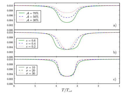
Fig. 1 : Influence of the hollow parameters on the conductivity profile for $K_{\hbox{max}}=10^{-2}$ and $T_{\hbox{bump}}/T_{\hbox{surf}}=3.5$.

2.1 Conditions for the instability

Using the well-known work integral formalism (e.g. Unno et al., 1989), it is easy to show that the following condition is necessary to get unstable modes by $\kappa$-mechanism in variable stars:

$$\dfrac{d{\cal K}_{T}}{dz}<0\quad\text{where}\quad{\cal K}_{T}\equiv\left(\dfrac{\partial\ln K_{0}}{\partial\ln T_{0}}\right)_{\rho_{0}}.$$ (2)

However, this condition is not sufficient as the ionisation region should also be located at a given location in the star, neither too deep nor too close to its surface. This area is the so-called transition region that separates the quasi-adiabatic interior from the strongly non-adiabatic surface and is defined by (e.g. Cox, 1980)

$$\Psi=\dfrac{\langle c_{v}T_{0}\rangle\Delta m}{\Pi L}\simeq 1,$$ (3)

where $\Delta m$ is the integrated mass between the considered point and the surface, $\Pi$ the mode period and $L$ the luminosity. $\Psi$ is the ratio between the thermal energy embedded between the given radius and the surface and the energy radiated during an oscillation period.

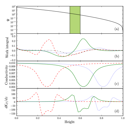
Fig. 2 : a) Vertical profile of the $\Psi$ coefficient (Eq. 3). The superimposed green zone represents the location where $\Psi=1\pm 0.5$. b) The real part of the work integral plotted for the three different equilibrium models. The dot-dashed black line is for the constant radiative conductivity case. c) Corresponding radiative conductivity profiles. d) Corresponding equilibrium fields $d{\cal K}_{T}/dz$ (Eq. 2).

2.2 The linear stability analysis

In order to check these two conditions, we perform a linear stability analysis by using the Linear Solver Builder code (Valdettaro et al., 2007). By starting with the conductivity profiles shown in Fig. 1, we first compute the equilibrium setup that is solution of both the hydrostatic and radiative equilibria given by

$$\vec{\nabla}p_{0}=\rho_{0}\vec{g}\quad\text{and}\quad\mathop{\hbox{div}}\nolimits[K_{0}(T_{0})\vec{\nabla}T_{0}]=0,$$ (4)

where $p_{0}$ and $\rho_{0}$ denote the equilibrium pressure and density. Then, we solve the linear oscillation equations for the perturbations by seeking normal modes of the form $\exp(\lambda t)$ with $\lambda=\tau+i\omega$, where $\omega$ is the mode frequency and $\tau$ its growth or damping rate (unstable modes corresponding to $\tau>0$). By varying the hollow parameters, we then determine the physical conditions that lead to unstable modes excited by the $\kappa$-mechanism in our layer (cf. Paper I).

The two criteria (2) and (3) predict that modes are unstable for a “sufficient” hollow (adequate amplitude and width) that is located in the transition region. Using the work integral computed from the obtained eigenvectors, we indeed recover instability strips for the $\kappa$-mechanism by considering the three different equilibrium setups (Fig. 2):

• The first case (dotted blue line, $T_{\hbox{bump}}/T_{\hbox{surf}}=1.7$) corresponds to a hot star with an ionisation region close to the surface. As the surrounding density is small, $\Psi\ll 1$ and the conductivity hollow hardly influences the work integral: driving is unable to prevail over damping, leading to $\tau<0$ or stable modes.

• In the second case (solid green line, $T_{\hbox{bump}}/T_{\hbox{surf}}=2.1$), the radiative conductivity begins to decrease significantly at the location of the transition region where $\Psi\simeq 1$. As a consequence, driving becomes important. Furthermore, the radiative conductivity increase occurs where non-adiabatic effects are already significant, i.e. $\Psi<1$ there. It means that no damping occurs between the hollow position and the surface as the radiative flux perturbations are frozen-in. Driving is overcoming damping in this case, therefore $\tau>0$ and modes are unstable.

• The third case (dashed red line, $T_{\hbox{bump}}/T_{\hbox{surf}}=2.8$) corresponds to a cold star of which ionisation region is located deeper in the stellar atmosphere where $\Psi\gg 1$. Ionisation then occurs in a quasi-adiabatic location. As a consequence, the excitation provided by the conductivity hollow cannot balance the damping arising at the top of the layer, thus $\tau<0$ and modes are stable.

In conclusion, our first radiative model of the $\kappa$-mechanism is well able to reproduce the main physics involved in the oscillations of Cepheid stars: (i) one should have $d{\cal K}_{T}/dz<0$ to drive the oscillations; (ii) the thermal engine underlying the conductivity hollow should also be located in the transition region where $\Psi\simeq 1$ (Fig. 2).

2.3 Study of the nonlinear saturation

To confirm both the results obtained previously in the linear stability analysis and to investigate the resulting nonlinear saturation, we perform direct numerical simulations of our problem. The idea is to start from the most favourable initial conditions found in the stability analysis and then advance the general hydrodynamic equations in time. We use a modified version of the public-domain finite-difference Pencil Code that includes an implicit solver of our own for the radiative diffusion term in the temperature equation (Gastine and Dintrans, 2008b, hereafter Paper II).

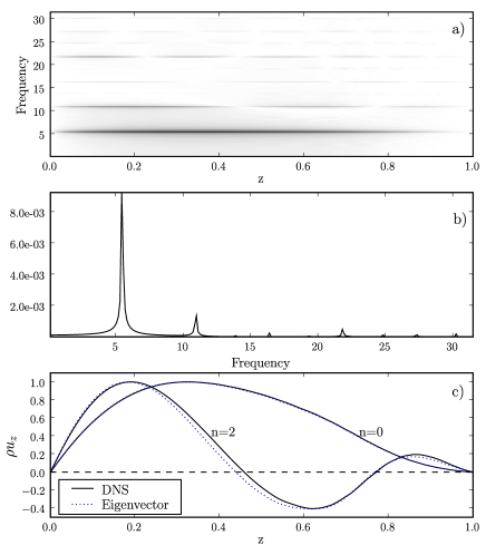
Fig. 3 : a) Temporal power spectrum for the momentum in the $(z,\ \omega)$-plane. b) The resulting spectrum after integrating over depth. c) Comparison between normalised momentum profiles for $n=(0,\ 2)$ modes according to the DNS power spectrum (solid black line) and to the linear stability analysis (dotted blue line).

To determine which modes are present in the DNS in the nonlinear-saturation regime, we first perform a temporal Fourier transform of the momentum field $\rho u(z,t)$ and plot the resulting power spectrum in the $(z,\omega)$-plane (Fig. 3a). The mean spectrum follows by integrating $\widehat{\rho u}(z,\omega)$ over depth (Fig. 3b). With this method, acoustic modes are extracted because they emerge as “shark-fin profiles” about definite eigenfrequencies (Dintrans and Brandenburg, 2004).

Several discrete peaks corresponding to normal modes well appear but the fundamental mode close to $\omega_{0}=5.439$ clearly dominates. Moreover, the linear eigenfunctions are compared to the mean profiles computed from a zoom taken in the DNS power spectrum about eigenfrequencies $\omega_{0}=5.439$ and $\omega_{2}=11.06$ (Fig. 3c). The agreement between the linear eigenfunctions (dotted blue lines) and the DNS profiles (solid black lines) is remarkable. In summary, Fig. 3 shows that several overtones are present in the DNS, even for long times. These overtones are however linearly stable suggesting that some underlying energy transfers occur between modes through nonlinear couplings.

These nonlinear interactions are investigated thanks to a tool that measures the sound generation by turbulent flows (e.g. Bogdan, Cattaneo, and Malagoli, 1993). It involves projections of the DNS physical fields onto the regular and adjoint eigenvectors that are solutions to the linear oscillation equations. The projection coefficients then give the time evolution of each acoustic mode that is present in the DNS separately. Furthermore, as the evolution of the kinetic energy of each mode is also accessible with this method, one can follow the energy transfer between modes.

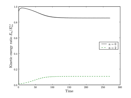
Fig. 4 : Time evolution of the kinetic energy ratio for the $n=0$ and $n=2$ acoustic modes.

Figure 4 shows an example of the time evolution of the kinetic energy ratio $E_{n}/E^{\text{tot}}_{\text{kin}}$ for the two modes $n=0$ (i.e. the fundamental one) and $n=2$ (i.e. the second overtone). Here $E_{n}$ denotes the kinetic energy embedded in the acoustic mode of order $n$, while $E^{\text{tot}}_{\text{kin}}$ is the total kinetic energy in the simulation. After its linear transient growth, a given fraction of the fundamental mode energy is progressively transferred to the second overtone until the nonlinear saturation is achieved above time $t\simeq 150$, with finally $85\%$ of the total kinetic energy in the $n=0$ mode and the remaining $15\%$ in the $n=2$ one. We recall that it is at a first glance surprising to detect this second overtone at long times because it is linearly stable and should normally be damped by diffusive effects.

The reason for its presence lies in a favored coupling in the period ratio between these two modes. Indeed, the fundamental period is $P_{0}=2\pi/\omega_{0}\simeq 1.155$ in this simulation while the $n=2$ one is $P_{2}\simeq 0.568$. As a consequence, the corresponding period ratio is close to one half ($P_{2}/P_{0}\simeq 0.491$) such that the second overtone is involved in the nonlinear saturation through a 2:1 resonance with the fundamental mode. The linear growth of the fundamental mode is then balanced by the pumping of energy to the stable second overtone that behaves as an energy sink, leading to the full limit-cycle stability.

3 Convective models in 2-D

3.1 From radiative to convective setups

After the previous results obtained on purely radiative models in 1-D, we next address the convection-pulsation coupling that is suspected to quench the radial oscillations of Cepheids close to the red edge. The idea is to slightly modify the unstable radiative setup to obtain a convective zone superimposed to the ionisation region in 2-D simulations. The convective instability obeys Schwarzschild’s criterion given by (e.g. Chandrasekhar, 1961)

$$\left|\dfrac{dT_{0}}{dz}\right|>\dfrac{g}{c_{p}}\quad\Longrightarrow\quad F_{\hbox{bot}}>\dfrac{gK_{0}(T_{0})}{c_{p}}.$$ (5)

where $F_{\hbox{bot}}=K_{0}|dT_{0}/dz|$ is the imposed bottom flux. For a given gravity $g$ and conductivity hollow $K_{0}(T_{0})$, convection will therefore develop for a large enough bottom flux satisfying Eq.(5).

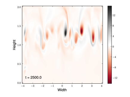
Fig. 5 : Snapshot of the vorticity field $\vec{\nabla}\times\vec{v}$ in a 2-D model with convection and $\kappa$-mechanism.

Figure 5 displays a snapshot of the vorticity field obtained in such a convective simulation at time $t=2500$. In order to ensure that the thermal relaxation is well achieved, we ran this simulation for a much longer time than in the purely-radiative case and the resolution is $256\times 256$ gridpoints. As expected, convection develops in the middle of the box where the conductivity hollow is located. Moreover, because of the density contrast across the convection zone, the vorticity is trapped in strong convective plume downdrafts that easily overshoot in the stable zone below due to their low Péclet number (Dintrans, 2009).

3.2 Evolution of acoustic modes with convection

To address the time evolution of the acoustic modes that are present in the DNS with convection, we project as before the physical fields onto an appropriate acoustic subspace to get the projection coefficient $c_{\ell n}(t)$. Here $\ell$ denotes the mode degree while $n$ is its order (with $k_{x}=(2\pi/L_{x})\ell$ and $L_{x}$ is the width of the box).

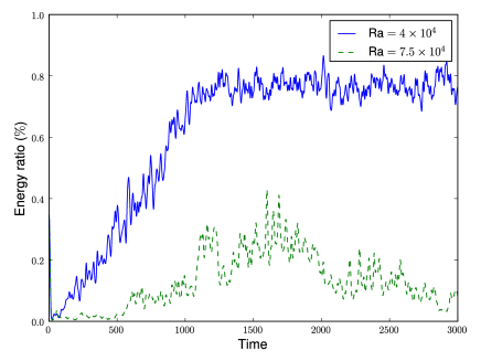
Fig. 6 : Evolution of the acoustic kinetic energy ratio for two simulations with a weak convection (solid blue line) and a stronger one (dashed green line).

Fig. 6 shows the total energy embedded in acoustic modes for two simulations with convection that differ by their Rayleigh number given by

$$\text{Ra}=-\dfrac{gd_{\text{conv}}^{4}}{\nu\chi c_{p}}\dfrac{ds}{dz}=\dfrac{(\nabla-\nabla_{\mbox{adia}})gd_{\text{conv}}^{4}}{\nu\chi H_{p}},$$ (6)

where $H_{p}=-(d\ln p_{0}/dz)^{-1}$ is the pressure scale height, $d_{\text{conv}}$ the vertical extent of the convection zone, $\chi=K_{0}/\rho_{0}c_{p}$ the radiative diffusivity and $s$ the entropy. This number allows to quantify the strength of the convective motions, that is, the critical Rayleigh number above which convection develops is about $10^{3}$ for polytropic stratifications (e.g. Gough et al., 1976).

In the first simulation ($\text{Ra}=4\times 10^{4}$, solid blue line), the Rayleigh number is slightly super-critical and the convection intensity is weak. In this case, we see that the acoustic energy ratio remains large (i.e. $\gtrsim 80\%$, the remaining $20\%$ being in the convection) and the nonlinear saturation is reached in the same way than in the previous radiative models. In other words, the mode propagation is not affected by convective motions and the convection can be seen as frozen-in.

On the contrary, increasing the Rayleigh number leads to a more vigorous convection and the acoustic energy ratio is much more affected by convective plumes (dashed green line). Indeed, after a long transient during which it reaches a non-trifling value ($\sim 30\%$), it progressively tends to zero at long times while the convective motions are responsible for the whole kinetic energy content. The radial oscillations excited by $\kappa$-mechanism are thus quenched by convection and this situation is relevant to the red edge where the unstable acoustic modes are known to be damped by convective motions occuring at the star’s surface.

We thus have shown that the Rayleigh number is a key parameter for this problem. But further investigations of the convection-pulsation coupling are in progress, by especially checking time-dependent theories of convection for which several free parameters can be constrained by such kind of direct numerical simulations (e.g. Yecko, Kolláth, and Buchler, 1998).

Acknowledgements Calculations were carried out on the CALMIP machine of the University of Toulouse (http://www.calmip.cict.fr/).

References

- Baker and Kippenhahn (1965) Baker, N., Kippenhahn, R.: Astrophys. J. 142, 868 (1965)
- Baker (1987) Baker, N.H.: In: Hillebrandt, W., Meyer-Hofmeister, E., Thomas, H.C. (eds.) Physical Processes in Comets, Stars and Active Galaxies, p. 105 (1987)
- Bogdan, Cattaneo, and Malagoli (1993) Bogdan, T.J., Cattaneo, F., Malagoli, A.: Astrophys. J. 407, 316 (1993)
- Bono, Marconi, and Stellingwerf (1999) Bono, G., Marconi, M., Stellingwerf, R.F.: Astrophys. J. Suppl. Ser. 122, 167 (1999)
- Chandrasekhar (1961) Chandrasekhar, S.: Hydrodynamic and hydromagnetic stability. Oxford University Press: Clarendon, Oxford (1961)
- Cox (1980) Cox, J.P.: Theory of stellar pulsation. Princeton University Press, Princeton (1980)
- Cox and Whitney (1958) Cox, J.P., Whitney, C.: Astrophys. J. 127, 561 (1958)
- Dintrans (2009) Dintrans, B.: Communications in Asteroseismology 158, 45 (2009)
- Dintrans and Brandenburg (2004) Dintrans, B., Brandenburg, A.: A&A 421, 775 (2004)
- Eddington (1917) Eddington, A.S.: The Observatory 40, 290 (1917)
- Gastine and Dintrans (2008a) Gastine, T., Dintrans, B.: Astron. Astrophys. 484, 29 (2008a)
- Gastine and Dintrans (2008b) Gastine, T., Dintrans, B.: Astron. Astrophys. 490, 743 (2008b)
- Gough et al. (1976) Gough, D.O., Moore, D.R., Spiegel, E.A., Weiss, N.O.: Astrophys. J. 206, 536 (1976)
- Unno et al. (1989) Unno, W., Osaki, Y., Ando, H., Saio, H., Shibahashi, H.: Nonradial oscillations of stars. University of Tokyo Press, Tokyo (1989)
- Valdettaro et al. (2007) Valdettaro, L., Rieutord, M., Braconnier, T., Fraysse, V.: JCoAM 205(1), 382 (2007)
- Yecko, Kolláth, and Buchler (1998) Yecko, P.A., Kolláth, Z., Buchler, J.R.: Astron. Astrophys. 336, 553 (1998)
- Zhevakin (1963) Zhevakin, S.A.: Annu. Rev. Astron. Astrophys. 1, 367 (1963)