A unified framework for mechanics.
Hamilton-Jacobi equation and applications

Abstract.

In this paper, we construct Hamilton-Jacobi equations for a great variety of mechanical systems (nonholonomic systems subjected to linear or affine constraints, dissipative systems subjected to external forces, time-dependent mechanical systems…). We recover all these, in principle, different cases using a unified framework based on skew-symmetric algebroids with a distinguished $1$-cocycle. Several examples illustrate the theory.

1. Introduction

A fundamental requirement for new developments in mechanics is to unravel the geometry that underlies different dynamical systems, especially mechanical systems. There are several reasons why this geometrical understanding is fundamental. First, it is a key tool for reduction by symmetries and for the geometric characterization of the integrability and stability theories. Second, the effective use of numerical techniques is often based on the comprehension of the fundamental structures appearing in the dynamics of mechanical and control systems. In fact, the geometrical analysis of such systems reveals what they have in common and indicates the most suitable strategy to analyze their solutions. Finally, the geometrical approach has provided substantial contributions to neighboring areas, such as molecular systems, classical field theories, control theory, engineering, etc.

Recent efforts have led to a unified framework for geometric mechanics based on a new structure, namely a Lie algebroid (see Section 2), which represents the phase space for lagrangian mechanics and whose dual is the phase space for hamiltonian mechanics. These ideas were introduced in a pioneering paper by A. Weinstein [41] (see also [25]) where the equations of motion were derived from a Lagrangian function given on a Lie algebroid. This was done using the linear Poisson structure on the dual of the Lie algebroid and the Legendre transformation associated with that regular Lagrangian. The unifying feature of the Lie-algebroid formalism is particularly relevant for the class of Lagrangian systems invariant under the action of a Lie group of symmetries (see [23] for a survey on the subject; see also [7, 29]).

As it turns out, the Lie-algebroid scheme is not general enough to include some interesting mechanical systems. On a Lie algebroid, the Jacobi identity for the bracket of sections implies the preservation of the associated linear Poisson bracket on its dual. However, many interesting examples are not covered by this strong assumption, for instance nonholonomic mechanics (see [5, 16, 20, 40] and references therein). Moreover, it would be interesting to find a general setting encompassing also some cases of dissipation of energy (for instance, explicit time-dependent systems, systems subjected to external forces or mechanical systems subjected to affine nonholonomic constraints). These reasons are our main motivation for introducing hamiltonian mechanics on more general objects, namely skew-symmetric algebroids equipped with a 1-cocycle; skew-symmetric algebroids will allow us to avoid the preservation of the Poisson bracket [3, 10, 12, 13, 22, 37] and the 1-cocycle will introduce a dissipative character to the dynamics (for the geometric description of time-dependent mechanics, in terms of Lie affgebroids or, equivalently, in terms of Lie algebroids with a 1-cocycle, see [11, 18, 19, 27, 28, 30]; see also [38]). Other approaches to the study of nonholonomic mechanical systems subjected to linear constraints, in the algebroid setting, have been also discussed in some recent papers (see [8, 9, 31, 32]). In these papers, the key tool is the notion of the prolongation of a Lie algebroid over a fibration.

Our main goal is to derive a Hamilton-Jacobi equation for the case of skew-symmetric algebroids with a 1-cocycle. As it is well known, Hamilton-Jacobi theory for unconstrained systems is a useful tool for the exact integration of Hamilton’s equations, for instance using the technique of separation of variables (see [1] and references therein). In other cases, this theory allows us to simplify the integration of Hamilton’s equations or, at least, to find some particular solutions of the system. To summarize the idea for classical Hamilton’s equations, consider a configuration manifold $Q$ and a hamiltonian $H:T^{*}Q\to\mathbb{R}$. Then the Hamilton-Jacobi equation can be written as

$$H(q,\frac{\partial W}{\partial q})=\hbox{constant}$$

for some function $W:Q\to\mathbb{R}$. If we find such a function $W$, then the integration of Hamilton’s equations (for initial condition along $dW(Q)$) is reduced to knowing the integral curves of a vector field on $Q$, defined as $X_{H}^{dW}=T\tau_{T^{*}Q}\circ X_{H}\circ dW\in{\mathfrak{X}}(Q)$, where $\tau_{T^{*}Q}:T^{*}Q\to Q$ is the canonical projection and $X_{H}$ is the hamiltonian vector field associated to $H$. Hence, from the integration of a vector field on the configuration space it is possible to recover some of the solutions of the original hamiltonian system.

A similar idea is also present in riemannian geometry when we look for a vector field $X\in{\mathfrak{X}}(Q)$ verifying $\nabla^{\mathcal{G}}_{X}X=0$ (a geodesic or auto-parallel vector field), where $\nabla^{\mathcal{G}}$ is the Levi-Civita connection associated to a riemannian metric ${\mathcal{G}}$ on $Q$. Their integral curves are geodesics, that is, solutions of the geodesic second-order differential equations corresponding to ${\mathcal{G}}$ with initial conditions on $\hbox{Im\;}X\subset TQ$. Observe that, in general, $X$ is not the gradient with respect to $\mathcal{G}$ of a function $W\in C^{\infty}(Q)$, which would be the case if we applied the classical Hamilton-Jacobi theorem. Hence, to recover this situation it is necessary to generalize the classical Hamilton-Jacobi equations.

On the other hand, recently, some of the authors of this paper proposed a generalization of the Hamilton-Jacobi equation for skew-symmetric algebroids (see [22]). Roughly speaking, a skew-symmetric algebroid is a vector bundle $\tau_{E}:E\longrightarrow Q$ equipped with a skew-symmetric bilinear bracket of sections and a vector bundle morphism, $\rho_{E}:E\to TQ$ (the anchor map), satisfying a Leibniz-type property, i.e., a Lie algebroid structure without the integrability property, (for more details, see Section 2). The existence of such a structure on $E$ is equivalent to the existence of a linear almost Poisson bracket on the dual bundle $\tau_{E^{*}}:E^{*}\to Q$, or the existence of an almost differential $d^{E}$ on $\tau_{E}:D\longrightarrow Q$ which satisfies all the properties of an standard differential except that $(d^{E})^{2}$ is not, in general, zero.

Skew-symmetric algebroids were used in [22] to describe the Hamilton-Jacobi equation of nonholonomic mechanical systems. In this case $E$ is determined by the linear constraints and the function $W\in C^{\infty}(Q)$ is replaced by a $1$-cocycle on the dual bundle $E^{*}$ (i.e., a section $\alpha$ of $E^{*}$ such that $d^{E}\alpha=0$). With these ideas, one derives a Hamilton-Jacobi equation for nonholonomic dynamics, illustrating the utility of this new theory for the integration of different nonholonomic problems. Hamilton-Jacobi theory for standard nonholonomic mechanical systems has been also discussed in recent papers (see [6, 17, 36]).

In this paper, we develop a Hamilton-Jacobi theory including, as particular cases, the Hamilton-Jacobi equation for skew-symmetric algebroids introduced in [22] and the case of auto-parallel vector fields in riemannian geometry (Example 4.3), as well as a great variety of new examples (time-dependent hamiltonian systems, systems with external forces, nonholonomic mechanics with affine constraints…). With this objective in mind, we obtain the main result of our paper, Theorem 3.1, the Hamilton-Jacobi equation for a hamiltonian system on a skew-symmetric algebroid with a $1$-cocycle. Moreover, our construction is preserved under the natural morphisms of the theory. This fact is proved in Theorem 3.6. We remark that this new version of the Hamilton-Jacobi equation is much more general than the one developed in [22], since here, we do not require the 1-section solutions of the Hamilton-Jacobi equation to be closed. This fact is extensively used in Example 4.12, where we find solutions for the problem of a rolling ball in a rotating plane with time-dependent angular velocity looking for functions $W\in C^{\infty}(Q)$ which do not satisfy $(d^{E})^{2}W=0$ (and thus, out of the cases studied in [22]). Moreover, the proof of the Theorem 3.1 is simpler and completely independent of the one done in [22].

The paper is structured as follows. In Section 2, we discuss some aspects of the geometry of skew-symmetric algebroids in the presence of a 1-cocycle. Moreover, given a hamiltonian section $h$ of the AV-bundle associated with the skew-symmetric algebroid and the 1-cocycle, we obtain Hamilton equations for $h$. In Section 3, we formulate and prove the Hamilton-Jacobi Theorem for a hamiltonian system on a skew-symmetric algebroid with a 1-cocycle. In addition, we see that the Hamilton-Jacobi equation is preserved under the natural morphisms of the theory. Finally, in the last section, some theoretical and practical examples will illustrate the power of these new techniques as for instance: Hamilton-Jacobi equation for a particle on a vertical cylinder in a uniform gravitational field with friction, for a homogeneous rolling ball without sliding on a rotating table with time-dependent angular velocity or for the vertical rolling disk with external forces.

2. Skew-symmetric algebroids, 1-cocycles and Hamiltonian dynamics

2.1. Skew-symmetric algebroids and 1-cocycles

Let $\tau_{E}:E\to Q$ be a vector bundle of rank $n$ over the manifold $Q$. We denote by $\Gamma(E)$ the $C^{\infty}(Q)$-module of sections of $E$. A skew-symmetric algebroid structure on $E$ is a pair $([\![\cdot,\cdot]\!],\rho)$, where $[\![\cdot,\cdot]\!]:\Gamma(E)\times\Gamma(E)\to\Gamma(E)$ is a $\mathbb{R}$-bilinear skew-symmetric bracket on $\Gamma(E)$ and $\rho:E\to TQ$ is a vector bundle map (the anchor map) such that

$$[\![\sigma,f\gamma]\!]=f[\![\sigma,\gamma]\!]+\rho(\sigma)(f)\gamma,\;\;\;\sigma,\gamma\in\Gamma(E),\;\;\;f\in C^{\infty}(Q).$$

Note that $\rho:E\to TQ$ induces a homomorphism of $C^{\infty}(Q)$-modules which we denote also by $\rho:\Gamma(E)\to{\mathfrak{X}}(Q)$ (see [3, 12, 14, 15, 22, 37]).

If the bracket $[\![\cdot,\cdot]\!]$ satisfies the Jacobi identity then $(E,[\![\cdot,\cdot]\!],\rho)$ is a Lie algebroid (see, for instance, [26]). In such a case, we have that the anchor map is a morphism of Lie algebras, i.e.

$$\rho([\![\sigma,\gamma]\!])=[\rho(\sigma),\rho(\gamma)],\mbox{ for }\sigma,\gamma\in\Gamma(E).$$

On a skew-symmetric algebroid structure $([\![\cdot,\cdot]\!],\rho)$ on the vector bundle $\tau_{E}:E\to Q$ it is induced the almost differential $d^{E}:\Gamma(\wedge^{\bullet}E^{*})\to\Gamma(\wedge^{\bullet+1}E^{*})$ as a $\mathbb{R}$-linear map given by

$$\begin{array}[]{rcl}(d^{E}f)(\sigma)&=&\rho(\sigma)(f),\\[8.0pt] (d^{E}\alpha)(\sigma,\gamma)&=&\rho(\sigma)(\alpha(\gamma))-\rho(\gamma)(\alpha(\sigma))-\alpha([\![\sigma,\gamma]\!])\end{array}$$ (2.1)

and

$$d^{E}(\beta_{1}\wedge\beta_{2})=d^{E}\beta_{1}\wedge\beta_{2}+(-1)^{k}\beta_{1}\wedge d^{E}\beta_{2},$$

for $f\in C^{\infty}(Q)$, $\alpha\in\Gamma(E^{*})$, $\sigma,\gamma\in\Gamma(E)$, $\beta_{1}\in\Gamma(\wedge^{k}E^{*})$ and $\beta_{2}\in\Gamma(\wedge^{\bullet}E^{*})$.

Note that $d^{E}$ is defined in a similar way that the standard differential over a manifold. However, there are important differences between them. In what follows, we will discuss some facts related with these differences.

Firstly, unlike the case of the stardard differential on a manifold, we have that the almost differential $d^{E}$ of a skew-symmetric algebroid $(E,[\![\cdot,\cdot]\!],\rho)$ is not, in general, a cohomology operator, i.e., $(d^{E})^{2}\not=0$. In fact, $(d^{E})^{2}=0$ if and only if $([\![\cdot,\cdot]\!],\rho)$ is a Lie algebroid structure.

For the particular case of a function $g\in C^{\infty}(Q)$, we deduce from (2.1) that $(d^{E})^{2}g=0$ if and only if $X(g)=0$ for all $X\in\widetilde{D}$, where $\widetilde{D}$ is the finitely generated distribution given by

$$\widetilde{D}:=span\{[\rho(\sigma),\rho(\gamma)]-\rho([\![\sigma,\gamma]\!])\ :\ \sigma,\gamma\in\Gamma(E)\}\subseteq\mathfrak{X}(Q).$$

On the other hand, if $Q$ is a connected manifold, in general, $d^{E}g=0$ does not imply that $g:Q\to{\mathbb{R}}$ is constant. In other words, if $Q$ is a connected manifold, in general, the vector space

$$H^{0}(d^{E})=\{f\in C^{\infty}(Q)\ \mbox{such that}\ d^{E}f=0\},$$

is not isomorphic to ${\mathbb{R}}.$ Note that, when $E$ is a Lie algebroid, $H^{0}(d^{E})$ is the Lie algebroid cohomology $0$-group of $E$. Even in this case, one can not guarantee that $H^{0}(d^{E})$ is isomorphic ${\mathbb{R}}$. However, if $Q$ is connected and $E$ is transitive, i.e., $\rho(E)=TQ$, then $H^{0}(d^{E})\cong{\mathbb{R}}$.

In [22] the authors discuss the relation between a function $g\in C^{\infty}(Q)$ being constant and $d^{E}g=0$. In order to remember these results we introduce the notion of completely nonholonomic distribution (see [33]).

Definition 2.1.

A distribution   ${\mathcal{D}}\subset TQ$  is called completely nonholonomic (or bracket generating) if $\{X_{k},[X_{k},X_{l}],[X_{i},[X_{k},X_{l}]],...\in\mathfrak{X}(Q)\ :\ X_{j}(q)\in{\mathcal{D}}_{q}\ \forall q\in Q\}$ spans the tangent bundle $TQ$.

The Lie brackets of vectors fields in ${\mathcal{D}}$ generate a flag ${\mathcal{D}}\subset{\mathcal{D}}^{2}\subset...\subset TQ$ with

$${\mathcal{D}}^{2}={\mathcal{D}}+[{\mathcal{D}},{\mathcal{D}}],\qquad{\mathcal{D}}^{r+1}={\mathcal{D}}^{r}+[{\mathcal{D}},{\mathcal{D}}^{r}]$$

where

$$[{\mathcal{D}},{\mathcal{D}}^{k}]=span\{[X,Y]\ :\ X\in{\mathcal{D}}\mbox{ and }Y\in{\mathcal{D}}^{k}\}$$

with the spans taken over smooth functions on $Q$ (for details, see [33]).

Here, we have two extreme cases: on one hand, the distribution ${\mathcal{D}}$ can be involutive, then we have ${\mathcal{D}}={\mathcal{D}}^{2}={\mathcal{D}}^{r},\ \forall r\in\mathbb{N}_{>0}.$ On the other hand, if ${\mathcal{D}}$ is completely nonholonomic, then there exists $r\in\mathbb{N}_{>0}$ such that ${\mathcal{D}}^{r}=TQ$.

Now, consider a skew-symmetric algebroid $(E,[\![\cdot,\cdot]\!],\rho)$ on a manifold $Q$ and the following finitely generated distribution ${\mathcal{D}}$ given by

$${\mathcal{D}}_{q}=\rho_{q}({E_{q}}),\;\;\;\mbox{ for all }q\in Q.$$

Proposition 2.2.

[22] If $(E,[\![\cdot,\cdot]\!],\rho)$ is a skew-symmetric algebroid over a connected manifold $Q$, such that ${\mathcal{D}}=\rho(E)\subset TQ$ is a completely nonholonomic distribution, then $H^{0}(d^{E})\cong\mathbb{R}$.

However, in some examples, the distribution ${\mathcal{D}}$ is not completely nonholonomic. In such a case there is $r\in\mathbb{N}_{>0}$ such that ${\mathcal{D}}^{r-1}\subsetneq{\mathcal{D}}^{r}={\mathcal{D}}^{r+1}\subsetneq TQ.$ This distribution ${\mathcal{D}}^{r}$ is the smallest Lie subalgebra of ${\mathfrak{X}}(Q)$ containing ${\mathcal{D}}$. Let us consider the associated generalized foliation over $Q.$ The leaf of this foliation over a point $q\in Q$, is just the orbit

$$L=\{\phi_{t_{k}}^{X_{k}}\circ...\circ\phi_{t_{1}}^{X_{1}}(q)\in Q\ :\ t_{i}\in\mathbb{R},\mbox{ and }X_{i}\in{\mathcal{D}}\mbox{ with }i=1,...,k,\ k\in\mathbb{N}_{>0}\}$$

where $\phi_{t_{i}}^{X_{i}}$ is the flow of the vector field $X_{i}$ at time $t_{i}$(see [2],[39]).

Theorem 2.3.

[22] Let $(E,[\![\cdot,\cdot]\!],\rho)$ be a skew-symmetric algebroid over a manifold $Q$. Consider the leaf $L$ of ${\mathcal{D}}^{r}$ as described above. Then

1. It is induced a skew-symmetric algebroid structure $([\![\cdot,\cdot]\!]_{L},\rho_{L})$ on the vector bundle $\tau_{L}:E_{L}\rightarrow L$ with $E_{L}:=\cup_{q\in L}E_{q}$. Moreover, the distribution $\rho_{L}(E_{L})$ on $L$ is completely nonholonomic.

2. If $f\in C^{\infty}(Q)$ is a function such that $d^{E}f=0$, then its restriction to $L$ is constant.

Next, we will see that any skew-symmetric algebroid structure $([\![\cdot,\cdot]\!],\rho)$ on the vector bundle $\tau_{E}:E\to Q$ induces an almost Poisson linear bracket $\{\cdot,\cdot\}:C^{\infty}(E^{*})\times C^{\infty}(E^{*})\to C^{\infty}(E^{*})$ on the space of functions on $E^{*}$, that is, $\{\cdot,\cdot\}$ is a skew-symmetric $\mathbb{R}$-bilinear bracket which is a derivation in each argument with respect to the standard product of functions and with the extra property that the bracket of two linear functions is again a linear function. Indeed, this bracket is characterized by the following relations (see [3, 12, 14, 15, 22])

$$\begin{array}[]{c}\{\widehat{{\sigma}},\widehat{{\gamma}}\}=-\widehat{[\![{\sigma},{\gamma}]\!]},\qquad\{f\circ\tau_{{E}^{*}},\widehat{\sigma}\}=\rho({\sigma})(f)\circ\tau_{{E}^{*}}\\[8.0pt] \{f\circ\tau_{{E}^{*}},g\circ\tau_{{E}^{*}}\}=0,\end{array}$$ (2.2)

for all $\sigma,\gamma\in\Gamma(E)$ and $f,g\in C^{\infty}(Q)$ and where $\widehat{\zeta}:E^{*}\to\mathbb{R}$ is the linear function associated with the section $\zeta\in\Gamma(E).$

Now, we will endow our skew-symmetric algebroid with an additional structure: a distinguished section $\phi\in\Gamma(E^{*})$ which allows us to consider some interesting examples.

Let us consider a section $\phi$ of $E^{*}$. Denote by $\phi^{\vee}\in{\mathfrak{X}}(E^{*})$ the vertical lift of the section $\phi\in\Gamma(E^{*})$, that is, the vector field defined by

$$\phi^{\vee}(\alpha)=(\phi(\tau_{E^{*}}(\alpha)))_{\alpha}^{\vee},\;\;\;\forall\alpha\in E^{*},$$

where $\;{}_{\alpha}^{\vee}:E^{*}_{\tau_{E^{*}}(\alpha)}\to T_{\alpha}(E^{*}_{\tau_{E^{*}}(\alpha)})$ is the canonical isomorphism between the vector spaces $E^{*}_{\tau_{E^{*}}(\alpha)}$ and $T_{\alpha}(E^{*}_{\tau_{E^{*}}(\alpha)}).$ Note that

$$\phi^{\vee}(\widehat{\sigma})=\phi(\sigma)\circ\tau_{E^{*}}=\widehat{\sigma}\circ\phi\circ\tau_{E^{*}},$$ (2.3)

for all $\sigma\in\Gamma(E)$.

Using (2.1), (2.2) and (2.3), we obtain the following formula which describes the differential of $\phi$ in terms of the linear bracket $\{\cdot,\cdot\}$ on $E^{*}$

$$\begin{array}[]{rcl}d^{E}\phi(\gamma,\sigma)\circ\tau_{E^{*}}&=&-(\{\phi^{\vee}(\widehat{\gamma}),\widehat{\sigma}\}+\{\widehat{\gamma},\phi^{\vee}(\widehat{\sigma})\}-\phi^{\vee}(\{\widehat{\gamma},\widehat{\sigma}\})\\[8.0pt] &=&-(\{\widehat{\gamma},\widehat{\sigma}\circ\phi\circ\tau_{E^{*}}\}-\{\widehat{\gamma},\widehat{\sigma}\}+\{\widehat{\gamma}\circ\phi\circ\tau_{E^{*}},\widehat{\sigma}\}),\end{array}$$ (2.4)

for all $\gamma,\sigma\in\Gamma(E)$. Thus, $\phi\in\Gamma(E^{*})$ is a $1$-cocycle, i.e., $d^{E}\phi=0$, if and only if

$$\phi^{\vee}(\{\varphi_{1},\varphi_{2}\})=\{\phi^{\vee}(\varphi_{1}),\varphi_{2}\}+\{\varphi_{1},\phi^{\vee}(\varphi_{2})\},$$ (2.5)

for all $\varphi_{1},\varphi_{2}\in C^{\infty}(E^{*})$. Moreover, equation (2.5) is equivalent to the fact that the linear bivector $\Pi_{E^{*}}$ on $E^{*}$ associated with the bracket $\{\cdot,\cdot\}$ is invariant with respect to the vector field $\phi^{\vee}\in{\mathfrak{X}}(E^{*})$, i.e.,

$${\mathcal{L}}_{\phi^{\vee}}\Pi_{E^{*}}=0.$$ (2.6)

In fact, from (2.2), (2.5) and (2.6) one may conclude the following result:

Proposition 2.4.

Let $\tau_{E}:E\to Q$ be a vector bundle over $Q$ and $\phi\in\Gamma(E^{*})$ a section of the dual bundle of $E$. Then, the following statements are equivalent:

1. $E$ admits a skew-symmetric algebroid structure $([\![\cdot,\cdot]\!],\rho)$ such that $d^{E}\phi=0$.

2. There is a linear bivector $\Pi_{E^{*}}$ on $E^{*}$ which is invariant with respect to the vertical lift $\phi^{\vee}\in{\mathfrak{X}}(E^{*})$ of $\phi$.

2.2. Hamiltonian dynamics

Let $(E,[\![\cdot,\cdot]\!],\rho)$ be a skew-symmetric algebroid over $Q$ of rank $n$, and $\phi\in\Gamma(E^{*})$ be a $1$-cocycle of $E$. Denote by $\widehat{\phi}:E\to\mathbb{R}$ the corresponding linear function induced by $\phi$ on $E$ and suppose that, for all $q\in Q,$ $\widehat{\phi}_{|E_{q}}\not=0.$ Then, one may consider the affine bundle

$$\tau_{\mathcal{A}}:{\mathcal{A}}:=\widehat{\phi}^{-1}(1)\to Q$$

of rank $n-1$ with associated vector bundle $\tau_{V}:V:=\widehat{\phi}^{-1}(0)\to Q.$ Note that $V$ is a skew-symmetric algebroid over $Q$ with structure $([\![\cdot,\cdot]\!]_{V},\rho_{V})$ given by

$$i_{V}\circ[\![\sigma,\gamma]\!]_{V}=[\![i_{V}(\sigma),i_{V}(\gamma)]\!],\;\;\;\rho_{V}(\sigma)=\rho(i_{V}(\sigma))$$

for all $\sigma,\gamma\in\Gamma(V)$, where $i_{V}:V\to E$ is the canonical inclusion. Thus, we have the corresponding linear almost Poisson 2-vector $\Pi_{V^{*}}$ on $V^{*}$.

On the other hand, the map $\mu:=i_{V}^{*}:E^{*}\to V^{*}$ defines an affine bundle of rank $1$ modeled over the trivial vector bundle $pr_{1}:V^{*}\times\mathbb{R}\to V^{*}$ (an AV-bundle in the terminology of [11]). Using (2.2) and the fact that the canonical inclusion $i_{V}:V\to E$ is a skew-symmetric algebroid monomorphism, we deduce that $\mu:E^{*}\to V^{*}$ is an almost Poisson morphism. Thus, if $\alpha_{q}\in E^{*}_{q}$, we have that the following diagram is commutative

Here, $\#_{\Pi_{E^{*}}}:T^{*}E^{*}\to TE^{*}$ (respectively, $\#_{\Pi_{V^{*}}}:T^{*}V^{*}\to TV^{*})$ is the morphism of $C^{\infty}(Q)$-modules induced by the almost Poisson bivector $\Pi_{E^{*}}$ (respectively, $\Pi_{V^{*}}$).

Using again (2.2), we also deduce that

$$d^{V}f=\mu\circ d^{E}f\mbox{ and }d^{V}(\mu\circ\alpha)=\wedge^{2}\mu\circ d^{E}\alpha,\;\;\;f\in C^{\infty}(M),\;\;\;\alpha\in\Gamma(E^{*}),$$

where $\wedge^{2}\mu:\wedge^{2}E^{*}\rightarrow\wedge^{2}V^{*}$ is the extension of $\mu$ to the corresponding vector bundles.

Note that the set of the global sections $\Gamma(\mu)$, of $\mu$, is an affine space modeled over $C^{\infty}(V^{*})$. In addition, if $h\in\Gamma(\mu)$ then $\mu(\alpha_{q}-h(\mu(\alpha_{q})))=0,$ for $q\in Q$ and $\alpha_{q}\in E^{*}_{q}$. Thus, one may define a function $F_{h}\in C^{\infty}(E^{*})$ characterized by

$$\alpha_{q}-h(\mu(\alpha_{q}))=F_{h}(\alpha_{q})\phi(q),$$ (2.7)

for all $q\in Q$ and for all $\alpha_{q}\in E^{*}_{q}$. Moreover, we have

$$(\phi^{\vee}(F_{h}))(\alpha_{q})=\left(\frac{d}{dt}_{|t=0}F_{h}(\alpha_{q}+t\phi(q))\right)=1.$$

Therefore, it follows that $\phi^{\vee}(F_{h})=1$. In fact, there is a one-to-one correspondence between $\Gamma(\mu)$ and the set of functions $F$ on $E^{*}$ which satisfy the relation

$$\phi^{\vee}(F)=1,$$ (2.8)

(see [11]).

In what follows, we will associate to each section $h\in\Gamma(\mu)$, a vector field on $V^{*}$. From (2.5) and (2.8), we deduce that, for every section $h$ of the bundle $\mu:E^{*}\to V^{*}$ and $G\in C^{\infty}(V^{*}),$ the function $\{G\circ\mu,F_{h}\}$ is $\mu$-projectable (note that $KerT_{\alpha_{q}}\mu=<\phi^{\vee}(\alpha_{q})>$). Thus, for each $h\in\Gamma(\mu)$ we can consider a vector field $R_{h}$ on $V^{*}$ which is characterized by

$$R_{h}(G)\circ\mu=\{G\circ\mu,F_{h}\},\;\;\;\;G\in C^{\infty}(V^{*}).$$ (2.9)

This vector field is called the hamiltonian vector field associated with the section $h$. If ${\mathcal{H}}^{\Pi_{E^{*}}}_{F_{h}}\in{\mathfrak{X}}(E^{*})$ is the hamiltonian vector field associated with the function $F_{h}\in C^{\infty}(E^{*})$ with respect to the linear almost Poisson bracket $\Pi_{E^{*}}$, i.e.,

$${\mathcal{H}}^{\Pi_{E^{*}}}_{F_{h}}=-i_{dF_{h}}\Pi_{E^{*}}$$

then, from (2.9), we deduce that

$$R_{h}\circ\mu=T\mu\circ{\mathcal{H}}_{F_{h}}^{\Pi_{E^{*}}}.$$ (2.10)

The integral curves of the vector field $R_{h}$ are the solutions of the Hamilton equations for $h$.

2.3. Local expressions

Let $E$ be a vector bundle on $Q$ of rank $n$, with a skew-symmetric algebroid structure $([\![\cdot,\cdot]\!],\rho)$.

Fixed a section $\phi$ of $E^{*}$ such that $d^{E}\phi=0$ and $\widehat{\phi}_{|E_{q}}\not=0$ for all $q\in Q$. Then it is induced a local basis $\{e_{0},e_{a}\}_{a=1,\dots,n-1}$ of $E$ adapted to the $1$- section $\phi$ in the sense that $\phi(e_{0})=1$ and $\phi(e_{a})=0.$ In terms of this basis we have the local structure functions, $\mathcal{C}_{ab}^{c},\rho_{a}^{i},\mathcal{C}_{0b}^{c},\rho_{0}^{i}\in C^{\infty}(Q)$ of $E$ defined by

$$[\![e_{a},e_{b}]\!]={\mathcal{C}}_{ab}^{c}e_{c},\quad[\![e_{0},e_{b}]\!]={\mathcal{C}}_{0b}^{c}e_{c}\quad\mbox{and}\quad\rho(e_{a})=\rho_{a}^{i}\frac{\partial}{\partial q^{i}},\quad\rho(e_{0})=\rho_{0}^{i}\frac{\partial}{\partial q^{i}}.$$

Note that the condition $d^{E}\phi=0$ implies that $\mathcal{C}_{ab}^{0}=0$, for all $a,b\in\{0,\dots,n-1\}$.

Moreover, with respect to the induced local coordinates $(q^{i},p_{0},p_{a})$ on $E^{*}$, the local expressions of the vector field $\phi^{\vee}\in{\mathfrak{X}}(E^{*})$ and the linear almost Poisson bivector $\Pi_{E^{*}}$ are

$$\begin{array}[]{rcl}\phi^{\vee}&=&\displaystyle\frac{\partial}{\partial p_{0}},\\ \Pi_{E^{*}}&=&\rho_{0}^{i}\displaystyle\frac{\partial}{\partial q^{i}}\wedge\displaystyle\frac{\partial}{\partial p_{0}}+\rho_{a}^{i}\displaystyle\frac{\partial}{\partial q^{i}}\wedge\displaystyle\frac{\partial}{\partial p_{a}}-\mathcal{C}_{0b}^{c}p_{c}\displaystyle\frac{\partial}{\partial p_{0}}\wedge\displaystyle\frac{\partial}{\partial p_{b}}-\displaystyle\frac{1}{2}\mathcal{C}_{ab}^{c}p_{c}\displaystyle\frac{\partial}{\partial p_{a}}\wedge\displaystyle\frac{\partial}{\partial p_{b}}.\end{array}$$

If $(q^{i},p_{a})$ are the corresponding coordinates of $V^{*},$ the local expression of $\mu:E^{*}\to V^{*}$ is

$$\mu(q^{i},p_{0},p_{a})=(q^{i},p_{a}).$$

Let $h:V^{*}\to E^{*}$ be a section of $\mu$ whose local expression is

$$h(q^{i},p_{a})=(q^{i},-H(q^{i},p_{b}),p_{a})$$

where $H$ is a local function of $V^{*}.$ Then the associated function $F_{h}:E^{*}\rightarrow\mathbb{R}$ is

$$F_{h}(q^{i},p_{0},p_{a})=p_{0}+H(q^{i},p_{a}).$$ (2.11)

Moreover, the local expression of the Hamiltonian vector field associated with this section $h:V^{*}\to E^{*}$ is given by

$$R_{h}=(\rho_{0}^{i}+\rho_{a}^{i}\frac{\partial H}{\partial p_{a}})\frac{\partial}{\partial q^{i}}+(-\rho_{b}^{i}\frac{\partial H}{\partial q^{i}}+(\mathcal{C}_{0b}^{c}+\mathcal{C}_{ab}^{c}\frac{\partial H}{\partial p_{a}})p_{c})\frac{\partial}{\partial p_{b}}.$$

Thus, the Hamilton equations are

$$\frac{dq^{i}}{dt}=\rho_{0}^{i}+\rho_{a}^{i}\frac{\partial H}{\partial p_{a}},\qquad\frac{dp_{b}}{dt}=-\rho_{b}^{i}\frac{\partial H}{\partial q^{i}}+(\mathcal{C}_{0b}^{c}+\mathcal{C}_{ab}^{c}\frac{\partial H}{\partial p_{a}})p_{c}.$$

A Lagrangian version of these equations was considered in [18] (see also [38]).

It is important to note that the previous dynamics on $V^{*}$ has a dissipative character. In fact, in the case when the AV-bundle $\mu:E^{*}\to V^{*}$ is trivial, then the local function $H$ is global and it is the hamiltonian function on $V^{*}$. In addition,

$$R_{h}(H)\circ\mu=\{H\circ\mu,F_{h}\}\not=0.$$

The local expression of this dissipative term is

$$\{H\circ\mu,F_{h}\}=\rho_{0}^{i}\frac{\partial H}{\partial q^{i}}+\mathcal{C}_{0b}^{c}p_{c}\frac{\partial H}{\partial p_{b}}.$$

2.4. Examples

Next, we will describe two interesting examples of skew-symmetric algebroids which will be useful for the mathematical description of the mechanical systems considered in this paper.

Example 2.5.

Consider a Lie algebroid structure $([\![\cdot,\cdot]\!],\rho)$ (or more generally a skew-symmetric algebroid structure) on a vector bundle $\tau_{\bar{E}}:{\bar{E}}\to Q$ of rank $n-1$ and $F:{\bar{E}}\to{\bar{E}}$ a homomorphism of vector bundles (over the identity of $Q$). Then, on the vector bundle $\tau_{\mathbb{R}\times{\bar{E}}}:\mathbb{R}\times\bar{E}\to Q$, it is induced a skew-symmetric algebroid structure $(E:=\mathbb{R}\times\bar{E},[\![\cdot,\cdot]\!]_{\mathbb{R}\times\bar{E}},\rho_{\mathbb{R}\times\bar{E}})$ given by

$$\begin{array}[]{rcl}[\![(f,\sigma),(g,\gamma)]\!]_{\mathbb{R}\times\bar{E}}&=&(\rho(\sigma)(g)-\rho(\gamma)(f),[\![\sigma,\gamma]\!]+gF(\sigma)-fF(\gamma)),\\[5.0pt] \rho_{\mathbb{R}\times\bar{E}}(f,\sigma)&=&\rho(\sigma),\end{array}$$ (2.12)

for all $(f,\sigma),(g,\gamma)\in\Gamma(E)=C^{\infty}(Q)\times\Gamma(\bar{E})\cong\Gamma(\mathbb{R}\times\bar{E})$.

Note that the space $\Gamma(\wedge^{2}(\mathbb{R}\times\bar{E}^{*}))$ may be identified with $\Gamma(\bar{E}^{*})\oplus\Gamma(\wedge^{2}\bar{E}^{*})$. Under this identification, for $(f,\alpha)\in C^{\infty}(Q)\times\Gamma(\bar{E}^{*})\cong\Gamma(\mathbb{R}\times\bar{E}^{*})$, we obtain that

$$\begin{array}[]{rcl}d^{\mathbb{R}\times\bar{E}}(f,\alpha)&=&(F^{*}\alpha-d^{\bar{E}}f,d^{\bar{E}}\alpha),\end{array}$$ (2.13)

where $F^{*}\alpha$ is a section of $\bar{E}^{*}$ defined by

$$(F^{*}\alpha)(\sigma)=\alpha(F(\sigma)),\,\;\;\forall\sigma\in\Gamma(\bar{E}).$$

From (2.13), we have that $(1,0)\in\Gamma(\mathbb{R}\times\bar{E}^{*})$ is a $1$-cocycle, and its vertical lift is just the vector field $\frac{\partial}{\partial p_{0}}$ on $\mathbb{R}\times\bar{E}^{*}$, with $p_{0}$ the global coordinate on $\mathbb{R}$.

In this case, the linear almost Poisson bivector on $\mathbb{R}\times\bar{E}^{*}$ is given by

$$\Pi_{\mathbb{R}\times\bar{E}^{*}}=\Pi_{\bar{E}^{*}}+\frac{\partial}{\partial p_{0}}\wedge(F^{*})^{\vee},$$

where $\Pi_{\bar{E}^{*}}$ is the linear Poisson bivector on $\bar{E}^{*}$ induced by the Lie algebroid structure on $\bar{E}$ and $(F^{*})^{\vee}$ is the vector field on $\bar{E}^{*}$ defined by

$$(F^{*})^{\vee}:\bar{E}^{*}\to T\bar{E}^{*},\;\;\;\ (F^{*})^{\vee}(\alpha)=F^{*}(\alpha)_{\alpha}^{\vee}.$$

Here, $F^{*}:\bar{E}^{*}\to\bar{E}^{*}$ is the dual morphism of $F:\bar{E}\to\bar{E}.$

On the other hand, the affine bundle associated with $(\mathbb{R}\times\bar{E},[\![\cdot,\cdot]\!]_{\mathbb{R}\times\bar{E}},\rho_{\mathbb{R}\times\bar{E}},(1,0))$ is just $\tau_{\{1\}\times\bar{E}}:\{1\}\times\bar{E}\cong\bar{E}\to Q$ with associated vector bundle $\tau_{\{0\}\times\bar{E}}:\{0\}\times\bar{E}\cong\bar{E}\to Q$.

Moreover, the associated AV-bundle $\mu:\mathbb{R}\times\bar{E}^{*}\to\bar{E}^{*}$ is just the trivial affine bundle over $\bar{E}^{*}$ of rank $1$. Therefore, there is a one-to-one correspondence between sections $h:\bar{E}^{*}\to\mathbb{R}\times\bar{E}^{*}$ of this affine bundle and functions $H:\bar{E}^{*}\to\mathbb{R}.$ Furthermore, the hamiltonian vector field associated with $h$ is just

$$R_{h}={\mathcal{H}}_{H}^{\Pi_{\bar{E}^{*}}}-(F^{*})^{\vee},$$ (2.14)

where ${\mathcal{H}}_{H}^{\Pi_{\bar{E}^{*}}}\in{\mathfrak{X}}(\bar{E}^{*})$ is the hamiltonian vector field associated with $H$ with respect to the linear Poisson structure $\Pi_{\bar{E}^{*}}.$

Note that, in this case, the dissipative term is given by

$$R_{h}(H)=-(F^{*})^{\vee}(H).$$

Now, we will give some expressions in coordinates of the above objects. Let us consider local coordinates $(q^{i})$ on the manifold $Q$ and a local basis $\{\bar{e}_{a}\}_{a=1,\dots,n-1}$ of $\Gamma(\bar{E}).$

A local basis of sections of ${E}=\mathbb{R}\times\bar{E}$ is $\{e_{0},e_{a}\}_{a=1,\ldots,n-1}$, where $e_{0}=(1,0)$ and $e_{a}=(0,\bar{e}_{a})$. Locally, the homomorphism of vector bundles $F:\bar{E}\to\bar{E}$ is given by the functions $F^{b}_{a}\in C^{\infty}(Q)$, where $F(e_{a})=F^{b}_{a}e_{b}$. Then,

$$\begin{array}[]{rclcrcl}[\![e_{0},e_{a}]\!]_{\mathbb{R}\times\bar{E}}&=&-F_{a}^{b}e_{b},&&[\![e_{a},e_{b}]\!]_{\mathbb{R}\times\bar{E}}&=&{\mathcal{C}}_{ab}^{c}e_{c}\\[8.0pt] \rho_{E}(e_{0})&=&0,&&\rho_{E}(e_{a})&=&\rho_{a}^{i}\frac{\partial}{\partial q^{i}}.\end{array}$$

The linear almost Poisson bivector on $E^{*}=\mathbb{R}\times\bar{E}^{*}$ is now:

$$\Pi_{E^{*}} = \rho_{a}^{i}\displaystyle\frac{\partial}{\partial q^{i}}\wedge\displaystyle\frac{\partial}{\partial p_{a}}+F_{b}^{c}p_{c}\displaystyle\frac{\partial}{\partial p_{0}}\wedge\displaystyle\frac{\partial}{\partial p_{b}}-\displaystyle\frac{1}{2}\mathcal{C}_{ab}^{c}p_{c}\displaystyle\frac{\partial}{\partial p_{a}}\wedge\displaystyle\frac{\partial}{\partial p_{b}}.$$

Given a hamiltonian function $H:\bar{E}^{*}\to\mathbb{R}$ then the Hamilton equations of motion are:

$$\frac{dq^{i}}{dt} = \rho^{i}_{a}\frac{\partial H}{\partial p_{a}}$$

$$\frac{dp_{b}}{dt} = -\rho^{i}_{b}\frac{\partial H}{\partial q^{i}}+\mathcal{C}^{c}_{ab}p_{c}\frac{\partial H}{\partial p_{a}}-F_{b}^{a}p_{a}$$

Example 2.6.

(see [22]) Let $(E,[\![\cdot,\cdot]\!],\rho)$ be a Lie algebroid on a manifold $Q$. Suppose that we have a vector subbundle $D$ of $E$ and a projector, i.e., a vector bundle morphism ${\mathcal{P}}:E\to D$ (over the identity of $Q$) such that ${\mathcal{P}}_{|D}=id.$ Denote by $i_{D}:D\to E$ the natural inclusion from $D$ to $E.$ Then, we may induce a skew-symmetric algebroid structure on $D$ as follows

$$[\![\sigma,\gamma]\!]_{D}={\mathcal{P}}([\![i_{D}\circ\sigma,i_{D}\circ\gamma]\!]),\;\;\;\rho_{D}(\sigma)=\rho(i_{D}\circ\sigma),$$

for all $\sigma,\gamma\in\Gamma(D)$. Note that, in general, $([\![\cdot,\cdot]\!]_{D},\rho_{D})$ is not a Lie algebroid structure on $D$.

3. Hamilton-Jacobi equation, skew-symmetric algebroids with a 1-cocycle and linear almost Poisson morphisms

3.1. Hamilton-Jacobi equation

Let $\tau_{E}:E\to Q$ be a vector bundle, of rank $n$, on the manifold $Q$ with a skew-symmetric algebroid structure $([\![\cdot,\cdot]\!],\rho).$

Consider $\phi\in\Gamma(E^{*})$ a $1$-cocycle of $E$ which satisfies the following condition:

$$\widehat{\phi}_{|E_{q}}\not=0,\mbox{ for all }q\in Q.$$

Then, as we have shown in Section 2.2, the vector bundle $\tau_{V}:V:=\widehat{\phi}^{-1}(0)\to Q$ of rank $n-1$ admits a skew-symmetric algebroid structure which we denote by $([\![\cdot,\cdot]\!]_{V},\rho_{V}).$

If $h$ is a section of the corresponding AV-bundle $\mu:E^{*}\to V^{*}$ then $(E,[\![\cdot,\cdot]\!],\rho,\phi,h)$ is said to be a Hamiltonian system on $E$.

In such a case, for each section $\alpha$ of $V^{*}$, one may define a vector field $R_{h}^{\alpha}$ on $Q$ as follows

$$R_{h}^{\alpha}=T\tau_{V^{*}}\circ R_{h}\circ\alpha,$$ (3.1)

where $R_{h}$ is the hamiltonian vector field associated with the section $h$.

On the other hand, we may introduce the following map

$$\widetilde{\;\;\;\;}:\Omega^{1}(E^{*})\to\Gamma(E),\;\;\;\omega\to\widetilde{\omega},$$

where $\widetilde{\omega}$ is characterized by

$$\beta(\widetilde{\omega})=\omega(\beta^{\vee})\circ h\circ\alpha,\qquad\mbox{for all}\ \beta\in\Gamma(E^{*}).$$ (3.2)

We remark that $\widetilde{\omega}\in\Gamma(E)$ since, if $f\in C^{\infty}(Q)$ then $(f\beta)^{\vee}=(f\circ\tau_{E^{*}})\beta^{\vee}$ and

$$\tau_{E^{*}}\circ h\circ\alpha=id.$$ (3.3)

Moreover, it follows that

$$\widetilde{d\widehat{\gamma}}=\gamma,\;\;\;\widetilde{d(f\circ\tau_{E^{*}})}=0,\;\;\;\mbox{ and }\;\;\;\widetilde{F\omega}=(F\circ h\circ\alpha)\widetilde{\omega},$$ (3.4)

for $\gamma\in\Gamma(E)$, $f\in C^{\infty}(Q)$, $F\in C^{\infty}(E^{*})$ and $\omega\in\Omega^{1}(E^{*})$. We will denote by $\zeta_{h}^{\alpha}$ the section of $E$ given by

$$\zeta_{h}^{\alpha}=\widetilde{dF_{h}}.$$ (3.5)

Now, we state the main result of this paper.

Theorem 3.1.

Let $(E,[\![\cdot,\cdot]\!],\rho,\phi,h)$ be a Hamiltonian system on $E$. If $\alpha\in\Gamma(V^{*})$, we have that the following statements are equivalent:

1. If $c:I\to Q$ is an integral curve of $R^{\alpha}_{h}\in{\mathfrak{X}}(Q)$ then $\alpha\circ c:I\to V^{*}$ is an integral curve of $R_{h}\in{\mathfrak{X}}(V^{*}).$

2. $\alpha\in\Gamma(V^{*})$ satisfies the Hamilton-Jacobi equation, i.e.,

   $$\mu\circ(i_{\zeta_{h}^{\alpha}}d^{E}(h\circ\alpha))=0.$$

Proof.

From (2.2), (2.4) and (3.3), we deduce that for all $\gamma,\sigma\in\Gamma(E)$

$$\begin{array}[]{rcl}d^{E}(h\circ\alpha)(\gamma,\sigma)&=&(\rho(\gamma)(\widehat{\sigma}\circ h\circ\alpha)\circ\tau_{E^{*}}+\{\widehat{\gamma},\widehat{\sigma}\}-\rho(\sigma)(\widehat{\gamma}\circ h\circ\alpha)\circ\tau_{E^{*}})\circ h\circ\alpha\\[5.0pt] &\kern-60.0pt=&\kern-40.0pt-\Pi_{E^{*}}(d\widehat{\gamma},(h\circ\alpha\circ\tau_{E^{*}})^{*}(d\widehat{\sigma}))\circ h\circ\alpha+\Pi_{E^{*}}(d\widehat{\gamma}-(h\circ\alpha\circ\tau_{E^{*}})^{*}(d\widehat{\gamma}),d\widehat{\sigma})\circ h\circ\alpha.\end{array}$$ (3.6)

Moreover, using (3.4), it follows that

$$0=d^{E}(h\circ\alpha)(\widetilde{d(f\circ\tau_{E^{*}})},\widetilde{dF})$$ (3.7)

and by (2.2), (3.3) we obtain also that

$$0 = -\Pi_{E^{*}}(d(f\circ\tau_{E^{*}}),(h\circ\alpha\circ\tau_{E^{*}})^{*}(dF))\circ h\circ\alpha\;$$

$$\ +\Pi_{E^{*}}(d(f\circ\tau_{E^{*}})-(h\circ\alpha\circ\tau_{E^{*}})^{*}(d(f\circ\tau_{E^{*}})),dF)\circ h\circ\alpha$$

for all $F\in C^{\infty}(E^{*})$ and $f\in C^{\infty}(Q).$

Therefore, from (3.3), (3.4), (3.6), (3.7) and (3.1), we conclude that for all $\omega_{1},\omega_{2}\in\Omega^{1}(E^{*})$

$$\begin{array}[]{rcl}d^{E}(h\circ\alpha)(\widetilde{\omega_{1}},\widetilde{\omega_{2}})&=&-\Pi_{E^{*}}(\omega_{1},(h\circ\alpha\circ\tau_{E^{*}})^{*}\omega_{2})\circ h\circ\alpha\\ &&+\Pi_{E^{*}}(\omega_{1}-(h\circ\alpha\circ\tau_{E^{*}})^{*}\omega_{1},\omega_{2})\circ h\circ\alpha.\end{array}$$ (3.9)

Next, we will denote by $i_{V}:V\to E$ the natural inclusion. Then, if $\sigma\in\Gamma(V)$, considering in (3.9) the particular case when $\omega_{1}=dF_{h}$ and $\omega_{2}=d(\widehat{\sigma}\circ\mu)=d(\widehat{i_{V}\circ\sigma})$, we have that

$$d^{E}(h\circ\alpha)(\zeta_{h}^{\alpha},i_{V}\circ\sigma)={\mathcal{H}}_{F_{h}}^{\Pi_{E^{*}}}(\widehat{\sigma}\circ\alpha\circ\tau_{V^{*}}\circ\mu)\circ h\circ\alpha-{\mathcal{H}}^{\Pi_{E^{*}}}_{F_{n}}(\widehat{\sigma}\circ\mu)\circ h\circ\alpha.$$

Note that $(h\circ\alpha\circ\tau_{E^{*}})^{*}(dF_{h})=0$ (see (2.7)).

Now, using (2.10) we conclude that

$$d^{E}(h\circ\alpha)(\zeta_{h}^{\alpha},i_{V}\circ\sigma)=(T\alpha\circ R_{h}^{\alpha})(\widehat{\sigma})-R_{h}(\widehat{\sigma})\circ\alpha.$$ (3.10)

Next, we remark that statement $(i)$ in the theorem is equivalent to

$$T\alpha\circ R_{h}^{\alpha}=R_{h}\circ\alpha.$$ (3.11)

So, if this relation holds then, from (3.10), we deduce that $\mu\circ(i_{\zeta_{h}^{\alpha}}d^{E}(h\circ\alpha))=0.$

Conversely, suppose that

$$d^{E}(h\circ\alpha)(\zeta_{h}^{\alpha},i_{V}\circ\sigma)=0,\;\,\;\;\mbox{ for all }\sigma\in\Gamma(V).$$ (3.12)

In order to prove (3.11), it is sufficient to see that the following two relations are satisfied:

1. $R_{h}^{\alpha}(\widehat{\sigma}\circ\alpha)=R_{h}(\widehat{\sigma})\circ\alpha,$ for all $\sigma\in\Gamma(V),$

2. $R_{h}^{\alpha}(f)=R_{h}(f\circ\tau_{V^{*}})\circ\alpha,$ for all $f\in C^{\infty}(Q)$.

Statement $(a)$ is a consequence of Eq. (3.1) and $(b)$ follows from (3.10) and (3.12). ∎

In what follows, we write the local expression of the Hamilton-Jacobi equation.

Consider local coordinates $(q^{i})$ on $Q$ and a local basis $\{e_{0},e_{a}\}_{a=1,\dots,n-1}$ of $\Gamma(E)$ adapted to the $1$-cocycle $\phi$ as in Subsection 2.3

Denote by $(q^{i},p_{0},p_{a})$ (respectively, $(q^{i},p_{a})$) the corresponding local coordinates on $E^{*}$ (respectively, $V^{*}$). Then, the section $\alpha:Q\to V^{*}$ and the hamiltonian section $h:V^{*}\to E^{*}$ are written in terms of these coordinates as

$$\alpha(q^{i})=(q^{i},\alpha_{a}(q^{i})),\,\;\;h(q^{i},p_{a})=(q^{i},-H(q^{i},p_{a}),p_{a}).$$

On the other hand, a 1-form $\omega\in\Omega^{1}(E^{*})$ can be written in these coordinates as $\omega=\omega^{i}dq^{i}+\omega^{a}dp^{a}+\omega^{0}dp_{0}$ with $\omega^{i},\omega^{a},\omega^{0}\in C^{\infty}(E^{*})$. Therefore, from (3.2) we obtain that the section $\widetilde{\omega}\in\Gamma(E)$ is given by

$$\widetilde{\omega}=(\omega^{a}\circ h\circ\alpha)\,e_{a}+(\omega^{0}\circ h\circ\alpha)\,e_{0}.$$

Thus,

$$\zeta_{h}^{\alpha}=\widetilde{dF_{h}}=e_{0}+(\frac{\partial H}{\partial p_{a}}\circ\alpha)e_{a}.$$ (3.13)

Now, from (2.1) and (3.13), the Hamilton Jacobi equation is given locally as follows

$$(\rho_{0}^{i}+\rho_{b}^{i}\frac{\partial H}{\partial p_{b}})\frac{\partial\alpha_{a}}{\partial q^{i}}+(\rho_{a}^{i}\frac{\partial H}{\partial q^{i}}-(C_{0a}^{c}-C_{ab}^{c}\frac{\partial H}{\partial p_{b}})\alpha_{c})=0,$$

for all $a=1,\dots,n-1.$

To finish this subsection, we will show some consequences of Theorem 3.1 which will be useful for the next examples.

Corollary 3.2.

Let $(E,[\![\cdot,\cdot]\!],\rho,\phi,h)$ be a Hamiltonian system on $E$. If $\beta\in\Gamma(E^{*})$, then the following statements are equivalent:

1. If $c:I\to Q$ is an integral curve of $R^{\mu\circ\beta}_{h}\in{\mathfrak{X}}(Q)$ then $\mu\circ\beta\circ c:I\to V^{*}$ is an integral curve of $R_{h}\in{\mathfrak{X}}(V^{*}).$

2. $\beta\in\Gamma(E^{*})$ satisfies the Hamilton-Jacobi equation, i.e.,

   $$\mu\circ i_{\zeta_{h}^{\mu\circ\beta}}d^{E}\beta+d^{V}(F_{h}\circ\beta)=0.$$

Proof.

Using (2.7), we deduce that the Hamilton-Jacobi equation for $\mu\circ\beta\in\Gamma(V^{*})$ is

$$\mu\circ(i_{\zeta_{h}^{\mu\circ\beta}}d^{E}(\beta-(F_{h}\circ\beta)\phi))=0.$$ (3.14)

Since $\phi$ is a $1$-cocycle then

$$d^{E}(\beta-(F_{h}\circ\beta)\phi)=d^{E}\beta-d^{E}(F_{h}\circ\beta)\wedge\phi.$$ (3.15)

On the other hand, from (3.2), it follows that

$$\phi(\zeta_{h}^{\mu\circ\beta})=1$$

and therefore, using (3.15), we obtain that (3.14) is equivalent to

$$\mu\circ i_{\zeta_{h}^{\mu\circ\beta}}d^{E}\beta+\mu\circ d^{E}(F_{h}\circ\beta)-(i_{\zeta_{h}^{\mu\circ\beta}}(d^{E}(F_{h}\circ\beta)))\mu\circ\phi=0.$$

Finally, the corollary is an immediate consequence of Theorem 3.1 and the relations

$$\mu\circ d^{E}(F_{h}\circ\beta)=d^{V}(F_{h}\circ\beta)\;\;\mbox{ and }\;\;\mu\circ\phi=0.$$

∎

Corollary 3.3.

Let $(E,[\![\cdot,\cdot]\!],\rho,\phi,h)$ be a Hamiltonian system on the vector bundle $\tau_{E}:E\to Q$ on the connected manifold $Q$. Suppose that the finitely generated distribution ${\mathcal{V}}$ defined by ${\mathcal{V}}_{q}:=\rho_{V}(V_{q})$ for all $q\in Q$, is a completely nonholonomic distribution. If $\beta\in\Gamma(E^{*})$ is a $1$-cocycle of $E^{*}$, then the following statements are equivalent:

1. If $c:I\to Q$ is an integral curve of $R^{\mu\circ\beta}_{h}\in{\mathfrak{X}}(Q)$ then $\mu\circ\beta\circ c:I\to V^{*}$ is an integral curve of $R_{h}\in{\mathfrak{X}}(V^{*}).$

2. $\beta\in\Gamma(E^{*})$ satisfies the Hamilton-Jacobi equation

   $$F_{h}\circ\beta=constant.$$

3.2. Linear almost Poisson morphisms and Hamilton-Jacobi equation

As we pointed out in the introduction, one important advantage of dealing with unconstrained hamiltonian systems on Lie algebroids, or constrained systems on skew-symmetric algebroids, is that reduction by symmetries can be naturally handled by considering morphisms between Lie algebroids [41] (see also [7]), or respectively morphism between skew-symmetric algebroids, [22]. In the following section we deal with morphisms between skew-symmetric algebroids with a 1-cocycle, in order to show that the Hamilton Jacobi equation is preserved by such morphisms.

Suppose that $\tau_{E}:E\to Q$ and $\tau_{\bar{E}}:\bar{E}\to\bar{Q}$ are vector bundles over $Q$ and $\bar{Q}$, respectively. Consider a vector bundle morphism $(\Psi,\psi)$ between $E^{*}$ and $\bar{E}^{*}$

Denote by $\wedge^{k}\Psi:\wedge^{k}E^{*}\to\wedge^{k}\bar{E}^{*}$ the corresponding vector bundle morphism on $\psi:Q\to\bar{Q},$ induced by the pair $(\Psi,\psi),$ between the vector bundles $\wedge^{k}E^{*}\to Q$ and $\wedge^{k}\bar{E}^{*}\to\bar{Q}$. A section $\alpha\in\Gamma(\wedge^{k}E^{*})$ is $(\Psi,\psi)$-related with a section $\bar{\alpha}\in\Gamma(\wedge^{k}\bar{E}^{*})$ if

$$\wedge^{k}\Psi\circ\alpha=\bar{\alpha}\circ\psi.$$

Definition 3.4.

Let $(E,[\![\cdot,\cdot]\!]_{E},\rho,\phi,h)$ and $(\bar{E},[\![\cdot,]\!]_{\bar{E}},\bar{\rho},\bar{\phi},\bar{h})$ be hamiltonian systems on $E$ and $\bar{E},$ respectively. Suppose that $(\Psi,\psi)$ is a vector bundle morphism between $E^{*}$ and $\bar{E}^{*}$. Then, the pair $(\Psi,\psi)$ is said to be a hamiltonian morphism if:

1. $(\Psi,\psi)$ is an almost Poisson morphism, that is,

   $$\{\bar{F_{1}}\circ\Psi,\bar{F_{2}}\circ\Psi\}_{E^{*}}=\{\bar{F}_{1},\bar{F}_{2}\}_{\bar{E}^{*}}\circ\Psi,\mbox{ for }\bar{F}_{1},\bar{F}_{2}\in C^{\infty}(\bar{E}^{*})$$

   where $\{\cdot,\cdot\}_{E^{*}}$ (respectively, $\{\cdot,\cdot\}_{\bar{E}^{*}}$) is the linear almost Poisson bracket on $E^{*}$ (respectively, $\bar{E}^{*}$);

2. $\phi$ and $\bar{\phi}$ are $(\Psi,\psi)-$related and

3. $F_{\bar{h}}\circ\Psi=F_{h}.$

Now, we prove the following result

Proposition 3.5.

Let $(E,[\![\cdot,\cdot]\!]_{E},\rho,\phi,h)$ and $(\bar{E},[\![\cdot,\cdot]\!]_{\bar{E}},\bar{\rho},\bar{\phi},\bar{h})$ be hamiltonian systems on $E$ and $\bar{E},$ respectively, and $(\Psi,\psi)$ be a hamiltonian morphism between $E^{*}$ and $\bar{E}^{*}$. Then:

1. There exists a linear almost Poisson morphism $\widehat{\Psi}:V^{*}\to\bar{V}^{*}$ (over $\psi$) such that the following diagram is commutative

   (3.16)

2. The vector fields $R_{h}\in{\mathfrak{X}}(V^{*})$ and $R_{\bar{h}}\in{\mathfrak{X}}(\bar{V}^{*})$ are $\widehat{\Psi}-$related, that is,

   $$R_{\bar{h}}\circ\widehat{\Psi}=T\widehat{\Psi}\circ R_{h}.$$

3. If $\alpha\in\Gamma(V^{*})$ and $\bar{\alpha}\in\Gamma(V^{*})$ are $(\widehat{\Psi},\psi)$-related then the vector fields $R_{h}^{\alpha}\in{\mathfrak{X}}(Q)$ and $R_{\bar{h}}^{\bar{\alpha}}\in{\mathfrak{X}}(\bar{Q})$ are $\psi$-related, that is,

   $$R_{\bar{h}}^{\bar{\alpha}}\circ\psi=T\psi\circ R_{h}^{\alpha}.$$

Proof.

$(i)$ Using that $(\Psi,\psi)$ is a vector bundle morphism and the fact that $\Psi\circ\phi=\bar{\phi}\circ\psi,$ it follows that there exists a vector bundle morphism $\widehat{\Psi}:V^{*}\to\bar{V}^{*}$ (over $\psi$) such that the diagram (3.16) is commutative. Moreover, since $\Psi,\mu$ and $\bar{\mu}$ are linear almost Poisson morphisms, we deduce that $\widehat{\Psi}$ also is a linear almost Poisson morphism.

$(ii)$ The condition $F_{\bar{h}}\circ\Psi=F_{h}$ implies that

$${\mathcal{H}}_{F_{\bar{h}}}^{\Pi_{\bar{E}^{*}}}\circ\Psi=T\Psi\circ{\mathcal{H}}_{F_{h}}^{\Pi_{E^{*}}}$$

(note that $\Psi$ is an almost Poisson morphism). Thus, from $(i)$ and $(2.12)$, we have that

$$R_{\bar{h}}\circ\widehat{\Psi}=T\widehat{\Psi}\circ R_{h}.$$

$(iii)$ Using $(i)$, (3.1) and the fact that $\widehat{\Psi}\circ\alpha=\bar{\alpha}\circ\psi,$ we conclude that the vector fields $R_{h}^{\alpha}$ and $R_{\bar{h}}^{\bar{\alpha}}$ are $\psi$-related. ∎

From Proposition 3.5, we deduce that following result

Theorem 3.6.

Let $(E,[\![\cdot,\cdot]\!]_{E},\rho,\phi,h)$ and $(\bar{E},[\![\cdot,\cdot]\!]_{\bar{E}},\bar{\rho},\bar{\phi},\bar{h})$ be hamiltonian systems on $E$ and $\bar{E}$, respectively, and $(\Psi,\psi)$ be a hamiltonian morphism between $E^{*}$ and $\bar{E}^{*}.$ If $\alpha\in\Gamma(V^{*})$ satisfies the Hamilton-Jacobi equation for $h$, $\bar{\alpha}\in\Gamma(\bar{V}^{*})$ is $(\Psi,\psi)$-related with $\alpha$ and $\psi$ is a surjective map then $\bar{\alpha}$ satisfies the Hamilton-Jacobi equation for $\bar{h}$.

Remark 3.7.

Let $(E,[\![\cdot,\cdot]\!]_{E},\rho,\phi,h)$ and $(\bar{E},[\![\cdot,\cdot]\!]_{\bar{E}},\bar{\rho},\bar{\phi},\bar{h})$ be hamiltonian systems on $E$ and $\bar{E}$, respectively, and $(\Psi,\psi)$ be a hamiltonian morphism between $E^{*}$ and $\bar{E}^{*}.$ Suppose that $\bar{\alpha}\in\Gamma(E^{*})$ is a $1$-cocycle of $\bar{E}^{*}$ such that $F_{\bar{h}}\circ\bar{\alpha}=constant.$ Then, if $\alpha\in\Gamma(E^{*})$ is a $1$-cocycle of $E^{*}$ which is $(\Psi,\psi)$-related with $\bar{\alpha}$, it is clear that $F_{h}\circ\alpha=constant$ and, therefore, $\alpha$ is a solution of the Hamilton-Jacobi equation for $h.$ $\diamond$

4. Examples

In this section we will apply our theory to two type of mechanical systems: uncontrained mechanical systems with a dissipative character (with linear external forces or time-dependent systems) and nonholonomic mechanical systems subjected to affine constraints. In the last part of the section we will discuss the case of a nonholonomic mechanical system with external linear forces.

4.1. Uncontrained mechanical systems with a dissipative character

4.1.1. Mechanical systems on Lie algebroids with linear external forces

(See Example 2.5). Let us consider a Lie algebroid structure (or more generally a skew-symmetric algebroid) $([\![\cdot,\cdot]\!],\rho)$ on a vector bundle $\tau_{\bar{E}}:{\bar{E}}\to Q$ and a homomorphism of vector bundles $F:{\bar{E}}\to{\bar{E}}$ (over the identity of $Q$). With these ingredients, it is induced on the vector bundle $\tau_{\mathbb{R}\times{\bar{E}}}:\mathbb{R}\times\bar{E}\to Q$, a skew-symmetric algebroid structure $(E:=\mathbb{R}\times\bar{E},[\![\cdot,\cdot]\!]_{\mathbb{R}\times\bar{E}},\rho_{\mathbb{R}\times\bar{E}})$ such that $(1,0)\in\Gamma(\mathbb{R}\times\bar{E}^{*})\cong C^{\infty}(M)\times\Gamma(\bar{E}^{*})$ is a $1$-cocycle.

Let $H:\bar{E}^{*}\to{\mathbb{R}}$ be a differentiable function (Hamiltonian function) on $\bar{E}^{*}.$ Denote by $h:\bar{E}^{*}\to{\mathbb{R}}\times\bar{E}^{*}$ the induced section of $\mu=pr_{2}:{\mathbb{R}}\times\bar{E}^{*}\to\bar{E}^{*}$ by $H$, i.e.,

$$h(\beta_{q})=(-H(\beta_{q}),\beta_{q}),\;\;\;\;\mbox{ for all $q\in Q$ and $\beta_{q}\in\bar{E}_{q}^{*}.$}$$

The vector field $R_{h}$ on $\bar{E}^{*}$ is just ${\mathcal{H}}_{H}^{\Pi_{\bar{E}^{*}}}-(F^{*})^{\vee}$ (see (2.14)). Moreover,

$$R_{h}^{\alpha}=T\tau_{\bar{E}^{*}}\circ{\mathcal{H}}_{H}^{\Pi_{\bar{E}^{*}}}\circ\alpha.$$

On the other hand, for each $\alpha\in\Gamma(\bar{E}^{*})$ one may define a section, $\zeta_{H}^{\alpha},$ of $\bar{E}$ as follows

$$\beta(\zeta_{H}^{\alpha})=\beta^{\vee}(H)\circ\alpha,$$

for $\beta\in\Gamma(\bar{E}^{*})$. Then, under the identification $\Gamma({\mathbb{R}}\times\bar{E})\cong C^{\infty}(Q)\times\Gamma(\bar{E})$, $\zeta_{h}^{\alpha}$ is just $(1,\zeta_{H}^{\alpha}).$ Thus, using Corollary 3.2 we conclude the following result

Corollary 4.1.

Let $(\bar{E},[\![\cdot,\cdot]\!],\rho)$ be a Lie algebroid (or more generally a skew-symmetric algebroid) with Hamiltonian function $H:\bar{E}^{*}\to{\mathbb{R}}$, and $F:{\bar{E}}\to{\bar{E}}$ be a vector bundle homomorphism. If $\alpha\in\Gamma(\bar{E}^{*})$, the following statements are equivalent:

1. If $c:I\to Q$ is an integral curve of $T\tau_{\bar{E}^{*}}\circ{\mathcal{H}}_{H}^{\Pi_{\bar{E}^{*}}}\circ\alpha\in{\mathfrak{X}}(Q)$ then $\alpha\circ c:I\to E^{*}$ is an integral curve of ${\mathcal{H}}_{H}^{\Pi_{\bar{E}^{*}}}-(F^{*})^{\vee}.$

2. $\alpha\in\Gamma(\bar{E}^{*})$ satisfies the Hamilton-Jacobi equation, i.e.,

   $$i_{\zeta_{H}^{\alpha}}d^{\bar{E}}\alpha+d^{\bar{E}}(H\circ\alpha)+F^{*}(\alpha)=0.$$

Remark 4.2.

1. When $\alpha$ is a $1$-cocycle and $F\equiv 0$, we recover the result of [22]. Applications of this result to nonholonomic mechanical systems subjected to linear constraints were discussed there. Note that in this case the dissipative term is zero.

2. In the particular case when $\bar{E}$ is the standard Lie algebroid $\tau_{TQ}:TQ\to Q$, then, using well-known results (see, for instance, [24]), we deduce that there exists a one-to-one correspondence between the vector bundle morphisms $F:TQ\to T^{*}Q$ (over the identity of $Q$) and the semi-basic $1$-forms on $TQ$ which are homogeneous of degree $1$. A semi-basic $1$-form $\beta:TQ\to T^{*}(TQ)$ on $TQ$ is said to be homogeneous of degree $1$ if ${\mathcal{L}}_{\Delta}\beta=\beta$, where $\Delta$ is the Liouville vector field on $TQ$. Indeed, if

   $$F(q^{i},\dot{q}^{i})=(q^{i},F_{j}^{i}(q)\dot{q}^{j})$$

   then the corresponding $1$-form $\beta$ on $TQ$ is given by

   $$\beta=(F_{j}^{i}(q)\dot{q}^{j})dq^{i}.$$

   Using this result and Corollary 4.1, we deduce Theorem 3.4 in [17] for the particular case when the semi-basic $1$-form $\beta$ on $TQ$ is homogeneous of degree $1$.

$\diamond$

Example 4.3.

Standard mechanical systems. Let $\bar{E}$ be the standard Lie algebroid $\tau_{TQ}:TQ\to Q$. In this case the differential $d^{\bar{E}}$ is the standard differential, $d$, on $Q.$ Suppose that $F\equiv 0$ and that $H:T^{*}Q\to\mathbb{R}$ is a hamiltonian function. If $\alpha$ is a $1$-form on $Q$ then the Hamilton-Jacobi equation is

$$i_{X_{H}^{\alpha}}d\alpha+d(H\circ\alpha)=0,$$ (4.1)

where $X_{H}^{\alpha}$ is the vector field on $Q$ defined by $X_{H}^{\alpha}(\beta)=\beta^{\vee}(H)\circ\alpha$, for all $\beta\in\Omega^{1}(Q).$

If $Q$ is connected and $S:Q\to\mathbb{R}$ is a function on $Q$, using the $1$-form $\alpha=dS$, we obtain the standard Hamilton-Jacobi equation on $Q$, i.e.,

$$H\circ dS=constant.$$

On the other hand, let ${\mathcal{G}}$ be a riemannian metric on a n-dimensional manifold $Q$, i.e, a positive-definite symmetric $(0,2)$-tensor on $Q$. The metric ${\mathcal{G}}$ induces the musical isomorphisms

$$\flat_{\mathcal{G}}:{\mathfrak{X}}(Q)\longrightarrow\Omega^{1}(Q),\qquad\flat_{\mathcal{G}}(X)(Y)={\mathcal{G}}(X,Y),$$

$$\sharp_{\mathcal{G}}:\Omega^{1}(Q)\longrightarrow{\mathfrak{X}}(Q),\qquad\sharp_{\mathcal{G}}(\alpha)=\flat_{\mathcal{G}}^{-1}(\alpha)$$

where $X,Y\in{\mathfrak{X}}(Q)$ and $\alpha\in\Omega^{1}(Q)$.

Associated with the metric ${\mathcal{G}}$ there is an affine connection $\nabla^{\mathcal{G}}$, the Levi-Civita connection, determined by:

$$\begin{array}[]{l}[X,Y]=\nabla^{\mathcal{G}}_{X}Y-\nabla^{\mathcal{G}}_{Y}X\quad\hbox{ (symmetry)}\\ X({\mathcal{G}}(Y,Z))={\mathcal{G}}(\nabla^{\mathcal{G}}_{X}Y,Z)+{\mathcal{G}}(Y,\nabla^{\mathcal{G}}_{X}Z)\quad\hbox{ (metricity)}\;,\end{array}$$

for every $X,Y,Z\in{\mathfrak{X}}(Q)$.

Considering a vector field $X\in{\mathfrak{X}}(Q)$ and the associated 1-form $\alpha=\flat_{\mathcal{G}}(X),$ we will analyze the meaning of the Hamilton-Jacobi Equation (4.1) for the Hamiltonian $H:T^{*}Q\to\mathbb{R}$ defined by $H(\eta_{q})=\frac{1}{2}{\mathcal{G}}^{*}(\eta_{q},\eta_{q}),$ where ${\mathcal{G}}^{*}$ is the induced metric on $T^{*}Q$ and $\eta_{q}\in T^{*}_{q}Q$. First, we observe that the section $\zeta_{H}^{\alpha}$ of $TQ$ is just the vector field $X$. Then, for $Y\in{\mathfrak{X}}(Q)$

$$d\alpha(X,Y)+Y(H\circ\alpha) = d(\flat_{\mathcal{G}}(X))(X,Y)+\frac{1}{2}Y({\mathcal{G}}(X,X))$$

$$= X({\mathcal{G}}(X,Y))-\frac{1}{2}Y({\mathcal{G}}(X,X))-{\mathcal{G}}(X,[X,Y])$$

$$= {\mathcal{G}}(\nabla^{\mathcal{G}}_{X}X,Y).$$

Therefore, the Hamilton-Jacobi equation (4.1) for the case of a Hamiltonian defined by a riemmanian metric is equivalent to the condition for auto-parallelism of vector fields, that is, vector fields $X\in{\mathfrak{X}}(Q)$ such that $\nabla^{\mathcal{G}}_{X}X=0$.

Thus, if we have a vector field $X$ which satisfies the auto-parallelism condition, each integral curve $c:I\to Q$ (which is a geodesic) induces a solution of the Hamilton equations of the mechanical system, which is just

$$\flat_{\mathcal{G}}(X)\circ c:I\to T^{*}Q.$$

Example 4.4.

The test particle under the gravitational interaction of two masses. Consider the problem of the motion of a particle moving under the gravitational effect of two masses $m_{1}$ and $m_{2}$, which in turn move in circular orbits about their common center of mass and are not influenced by the motion of the particle (classical planar circular restricted three-body problem). Take a coordinate system rotating about the common center of mass with the same frequency as the two masses so that both of them lie on the $x$-axis with coordinates $(-\mu_{2},0)$ and $(\mu_{1},0)$, where $\mu_{i}=\frac{m_{i}}{m_{1}+m_{2}}$ (see [21, 34]).

The system is described by the Lagrangian function:

$$L(x,y,\dot{x},\dot{y})=\frac{1}{2}(\dot{x}-y)^{2}+\frac{1}{2}(\dot{y}+x)^{2}-\frac{\mu_{1}}{r_{1}}-\frac{\mu_{2}}{r_{2}},$$

where $r^{2}_{1}=(x+\mu_{2})^{2}+y^{2}$ and $r^{2}_{2}=(x-\mu_{1})^{2}+y^{2}$.

The equations of motion adding a drag force $\tilde{F}=(\tilde{F}_{1}(x,y,\dot{x},\dot{y}),\tilde{F}_{2}(x,y,\dot{x},\dot{y}))$ are (see [34]):

$$\ddot{x}-2\dot{y}-x = -\frac{\partial U}{\partial x}-\tilde{F}_{1},$$

$$\ddot{y}+2\dot{x}-y = -\frac{\partial U}{\partial y}-\tilde{F}_{2},$$

where $U(x,y)=\frac{\mu_{1}}{r_{1}}+\frac{\mu_{2}}{r_{2}}$ and $\tilde{F}:T\mathbb{R}^{2}\to T^{*}\mathbb{R}^{2}$.

Now, we will describe this system in our geometric framework. Consider the homomorphism $F:T\mathbb{R}^{2}\to T\mathbb{R}^{2}$ given by

$$F(\frac{\partial}{\partial x}) = F^{1}_{1}(x,y)\frac{\partial}{\partial x}+F^{2}_{1}(x,y)\frac{\partial}{\partial y},$$

$$F(\frac{\partial}{\partial y}) = F^{1}_{2}(x,y)\frac{\partial}{\partial x}+F^{2}_{2}(x,y)\frac{\partial}{\partial y},\$$

where $F^{a}_{b}\in C^{\infty}(\mathbb{R}^{2})$. Then, on the vector bundle $\tau:\mathbb{R}\times T\mathbb{R}^{2}\rightarrow\mathbb{R}^{2}$ it is induced a (transitive) skew-symmetric algebroid structure described, in the local basis $\{e_{0}=(1,0),e_{1}=(0,\frac{\partial}{\partial x}),e_{2}=(0,\frac{\partial}{\partial y})\}$, as follows

$$\begin{array}[]{c}[\![(1,0),(0,\displaystyle\frac{\partial}{\partial x})]\!]_{\mathbb{R}\times T\mathbb{R}^{2}}=(0,-F(\displaystyle\frac{\partial}{\partial x})),\;\;\;[\![(1,0),(0,\displaystyle\frac{\partial}{\partial y})]\!]_{\mathbb{R}\times T\mathbb{R}^{2}}=(0,-F\displaystyle(\frac{\partial}{\partial y})),\\[8.0pt] \rho_{\mathbb{R}\times T\mathbb{R}^{2}}(1,0)=0,\;\;\;\rho_{\mathbb{R}\times T\mathbb{R}^{2}}(0,\displaystyle\frac{\partial}{\partial x})=\displaystyle\frac{\partial}{\partial x},\;\;\;\rho_{\mathbb{R}\times T\mathbb{R}^{2}}(0,\displaystyle\frac{\partial}{\partial y})=\displaystyle\frac{\partial}{\partial y}.\end{array}$$

Therefore, $\mathcal{C}_{01}^{1}=-F^{1}_{1}$, $\mathcal{C}_{01}^{2}=-F^{2}_{1}$, $\mathcal{C}_{02}^{1}=-F^{1}_{2}$, $\mathcal{C}_{02}^{2}=-F^{2}_{2}$, $\rho^{1}_{1}=1$ and $\rho^{2}_{2}=1$.

Note that the homomorphism $F$ generates a drag force $\tilde{F}$ of the type

$$\tilde{F}(x,y,\dot{x},\dot{y}) = \left(F^{1}_{1}(x,y)\frac{\partial L}{\partial\dot{x}}+F^{2}_{1}(x,y)\frac{\partial L}{\partial\dot{y}},F^{1}_{2}(x,y)\frac{\partial L}{\partial\dot{x}}+F^{2}_{2}(x,y)\frac{\partial L}{\partial\dot{y}}\right)$$

$$= \left(F^{1}_{1}(x,y)(\dot{x}-y)+F^{2}_{1}(x,y)(\dot{y}+x),F^{1}_{2}(x,y)(\dot{x}-y)+F^{2}_{2}(x,y)(\dot{y}+x)\right).$$

On the dual bundle $\mathbb{R}\times T^{*}\mathbb{R}^{2}$ we have a hamiltonian function:

$$H(x,y,p_{x},p_{y})=\frac{1}{2}p_{x}^{2}+\frac{1}{2}p_{y}^{2}+yp_{x}-xp_{y}+U(x,y)$$ (4.2)

and the corresponding Hamilton’s equations are now:

$$\dot{x} = p_{x}+y,$$

$$\dot{y} = p_{y}-x,$$

$$\dot{p}_{x} = p_{y}-\frac{\partial U}{\partial x}-F_{1}^{1}(x,y)p_{x}-F_{1}^{2}(x,y)p_{y}=-\frac{\partial H}{\partial x}-F_{1}^{1}(x,y)p_{x}-F_{1}^{2}(x,y)p_{y},$$

$$\dot{p}_{y} = -p_{x}-\frac{\partial U}{\partial y}-F_{2}^{1}(x,y)p_{x}-F_{2}^{2}(x,y)p_{y}=-\frac{\partial H}{\partial y}-F_{2}^{1}(x,y)p_{x}-F_{2}^{2}(x,y)p_{y}.$$

Consider a section $\alpha\in\Gamma(T^{*}\mathbb{R}^{2})$ where $\alpha=\alpha_{1}\,dx+\alpha_{2}\,dy$. Then,

$$\zeta_{H}^{\alpha}=(\frac{\partial H}{\partial p_{x}}\circ\alpha)\frac{\partial}{\partial x}+(\frac{\partial H}{\partial p_{y}}\circ\alpha)\frac{\partial}{\partial y}$$

Thus, Hamilton-Jacobi equation is equivalent to

$$\frac{\partial H}{\partial x}\circ\alpha+(\frac{\partial H}{\partial p_{x}}\circ\alpha)\frac{\partial\alpha_{1}}{\partial x}+(\frac{\partial H}{\partial p_{y}}\circ\alpha)\frac{\partial\alpha_{1}}{\partial y}+\alpha_{i}F^{i}_{1} = 0$$

$$\frac{\partial H}{\partial y}\circ\alpha+(\frac{\partial H}{\partial p_{x}}\circ\alpha)\frac{\partial\alpha_{2}}{\partial x}+(\frac{\partial H}{\partial p_{y}}\circ\alpha)\frac{\partial\alpha_{2}}{\partial y}+\alpha_{i}F^{i}_{2} = 0\,.$$

For a hamiltonian function given by (4.2), the last two equations can be written as:

$$\frac{\partial U}{\partial x}-\alpha_{2}+(\alpha_{1}+y)\frac{\partial\alpha_{1}}{\partial x}+(\alpha_{2}-x)\frac{\partial\alpha_{1}}{\partial y}+\alpha_{i}F^{i}_{1} = 0$$

$$\frac{\partial U}{\partial y}+\alpha_{1}+(\alpha_{1}+y)\frac{\partial\alpha_{2}}{\partial x}+(\alpha_{2}-x)\frac{\partial\alpha_{2}}{\partial y}+\alpha_{i}F^{i}_{2} = 0\,.$$

An interesting case [34] is when the drag force is

$$\tilde{F}(x,y,\dot{x},\dot{y})=\left(k(x,y)(\dot{x}-y),k(x,y)(\dot{y}+x)\right),$$

with $k\in C^{\infty}(\mathbb{R}^{2})$. In this case, the homomorphism is $F(X)=k(x,y)X$ with $X\in T_{(x,y)}\mathbb{R}^{2}$. Thus, the equations of motion are

$$\dot{x} = p_{x}+y,$$

$$\dot{y} = p_{y}-x,$$

$$\dot{p}_{x} = p_{y}-\frac{\partial U}{\partial x}-k(x,y)p_{x},$$

$$\dot{p}_{y} = -p_{x}-\frac{\partial U}{\partial y}-k(x,y)p_{y}.$$

In this particular case the linear almost Poisson tensor on $\mathbb{R}\times T^{*}\mathbb{R}^{2}$ is given by

$$\Pi_{\mathbb{R}\times T^{*}\mathbb{R}^{2}}=\frac{\partial}{\partial x}\wedge\frac{\partial}{\partial p_{x}}+\frac{\partial}{\partial y}\wedge\frac{\partial}{\partial p_{y}}+k(x,y)p_{x}\frac{\partial}{\partial p_{0}}\wedge\frac{\partial}{\partial p_{x}}\\ +k(x,y)p_{y}\frac{\partial}{\partial p_{0}}\wedge\frac{\partial}{\partial p_{y}}$$

where $(p_{0},x,y,p_{x},p_{y})$ are standard coordinates on $\mathbb{R}\times T^{*}\mathbb{R}^{2}$.

Now, if the function $k$ is constant and we choose a section $\alpha=dS$ where $S:\mathbb{R}^{2}\to\mathbb{R}$ is an arbitrary function, the Hamilton-Jacobi equation is

$$d(H\circ\alpha)+kdS=0,$$

which is equivalent to the suggestive equation:

$$kS+H\circ dS=\hbox{constant}$$

or, in other words,

$$kS(x,y)+H(x,y,\frac{\partial S}{\partial x},\frac{\partial S}{\partial y})=\hbox{constant}.$$

In particular, for the hamiltonian function given by (4.2), we obtain the following partial differential equation:

$$kS(x,y)+\frac{1}{2}\left(\frac{\partial S}{\partial x}\right)^{2}+\frac{1}{2}\left(\frac{\partial S}{\partial y}\right)^{2}+y\frac{\partial S}{\partial x}-x\frac{\partial S}{\partial y}+U(x,y)=\hbox{constant}.$$

Note that, this equation is the Hamilton-Jacobi equation as stated in Corollary 3.3 for the cocycle $(kS,dS)\in C^{\infty}(\mathbb{R}^{2})\times\Omega^{1}(\mathbb{R}^{2})\simeq\Gamma((\mathbb{R}\times T\mathbb{R}^{2})^{*})$ when we consider the skew-symmetric algebroid $\tau:\mathbb{R}\times T\mathbb{R}^{2}\rightarrow\mathbb{R}^{2}$

Example 4.5.

Hamilton-Jacobi equation for a particle on a vertical cylinder in a uniform gravitational field with friction. As another example we consider a particle of mass $m$ constrained to move on a cylinder of radius $r$ in a uniform gravitational field of strength $g$ and assume also the existence of a frictional force acting on the system.

The Hamiltonian $H:T^{*}(\mathbb{R}\times S^{1})\to\mathbb{R}$ is:

$$H(x,\theta,p_{x},p_{\theta})=\frac{p_{x}^{2}}{2m}+\frac{p_{\theta}^{2}}{2mr^{2}}+mgx\;.$$

The frictional force is modeled in our setting by the homomorphism $F:T(\mathbb{R}\times S^{1})\to T(\mathbb{R}\times S^{1})$ given by

$$F(\frac{\partial}{\partial x}) = K_{1}\frac{\partial}{\partial x},$$

$$F(\frac{\partial}{\partial\theta}) = K_{2}\frac{\partial}{\partial\theta}\;,$$

with $(K_{1},K_{2})\in\mathbb{R}^{2}$.

The corresponding equations of motion are

$$m\dot{x} = p_{x}$$

$$mr^{2}\dot{\theta} = p_{\theta}$$

$$\dot{p}_{x} = -mg-K_{1}p_{x}$$

$$\dot{p}_{\theta} = -K_{2}p_{\theta}\;.$$

In this case, we may consider the skew-symmetric algebroid $\tau:\mathbb{R}\times T(\mathbb{R}\times S^{1})\to\mathbb{R}\times S^{1}$ associated with the above homomorphism $F:T(\mathbb{R}\times S^{1})\to T(\mathbb{R}\times S^{1})$ defined as in (2.12). For this skew-symmetric algebroid we have that $\phi=(1,0)\in\Gamma(\mathbb{R}\times T^{*}(\mathbb{R}\times S^{1}))=C^{\infty}(\mathbb{R}\times S^{1})\times\Omega^{1}(\mathbb{R}\times S^{1})$ is a 1-cocycle and $V=\widehat{\phi}^{-1}(0)=T(\mathbb{R}\times S^{1})$.

Let us consider a $1$-form $\alpha\in\Gamma(T^{*}(\mathbb{R}\times S^{1}))$. If locally $\alpha$ is given by

$$\alpha=\alpha_{x}dx+\alpha_{\theta}d\theta$$

with $\alpha_{x},\alpha_{\theta}\in C^{\infty}(\mathbb{R}\times S^{1})$, then the local expression of the vector field $\zeta_{H}^{\alpha}$ on $\mathbb{R}\times S^{1}$ is

$$\zeta_{H}^{\alpha}=\frac{\alpha_{x}}{m}\frac{\partial}{\partial x}+\frac{\alpha_{\theta}}{m}\frac{\partial}{\partial\theta}.$$

Moreover, the Hamilton-Jacobi equation for $\alpha\in\Omega^{1}(\mathbb{R}\times S^{1})$ is

$$i_{\zeta_{H}^{\alpha}}d\alpha+d(H\circ\alpha)+F^{*}\alpha=0,$$

where $d$ is the standard differential and $F^{*}\alpha$ is the pullback of $\alpha$ by $F$ (see Example 2.5). In local coordinates this equation becomes

$$\frac{\alpha_{x}}{m}\frac{\partial\alpha_{x}}{\partial x}+\frac{\alpha_{\theta}}{mr^{2}}\frac{\partial\alpha_{x}}{\partial\theta}+mg+K_{1}\alpha_{x} = 0,$$

$$\frac{\alpha_{x}}{m}\frac{\partial\alpha_{\theta}}{\partial x}+\frac{\alpha_{\theta}}{mr^{2}}\frac{\partial\alpha_{\theta}}{\partial\theta}+K_{2}\alpha_{\theta} = 0.$$

In the particular case when $\alpha=dS$ with $S$ a function given by $S(x,\theta)=S^{(1)}(x)+S^{(2)}(\theta)$, we have that the corresponding Hamilton-Jacobi equation is

$$K_{1}\frac{dS^{(1)}}{dx}+mg+\frac{1}{m}\frac{dS^{(1)}}{dx}\frac{d^{2}S^{(1)}}{dx^{2}} = 0,$$

$$K_{2}\frac{dS^{(2)}}{d\theta}+\frac{1}{mr^{2}}\frac{dS^{(2)}}{d\theta}\frac{d^{2}S^{(2)}}{d\theta^{2}} = 0\;.$$

Solving the equation we obtain that

$$S^{(2)}(\theta) = 0\hbox{ or }S^{(2)}(\theta)=-\frac{K_{2}mr^{2}}{2}\theta^{2}+C_{1}$$

$$S^{(1)}(x) = \frac{-gm-gm\mathbf{W}\left[\displaystyle{-\frac{e^{-1+\frac{K_{1}^{2}x}{g}-\frac{K_{1}^{2}C_{2}}{gm}}}{gm}}\right]}{K_{1}}\hbox{ if $K_{1}\not=0$ or }$$

$$S^{(1)}(x) = \pm\sqrt{2}\sqrt{-gm^{2}x+C_{2}}\hbox{ if $K_{1}=0$}\;,$$

where $\mathbf{W}$ is the Lambert W-function (the inverse function of $f(v)=ve^{v}$) and $C_{1}$ and $C_{2}$ are constants.

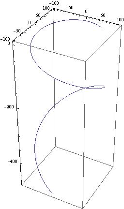
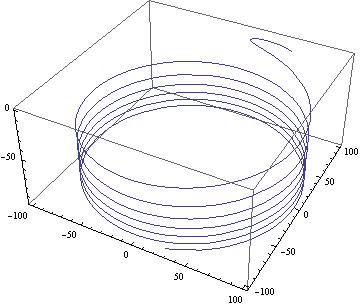
Figure 1. Comparison of a free trajectory (without friction), on the left, and a trajectory with friction, on the right

In Figure $1$, we compare the trajectory of the particle for the free problem and the trajectory for the problem with friction.

4.1.2. Unconstrained mechanical systems on Lie algebroids with a 1-cocycle

Let $([\![\cdot,\cdot]\!],\rho)$ be a Lie algebroid structure (or more generally a skew-symmetric algebroid) on a vector bundle $\tau_{E}:E\to Q$ and $\phi\in\Gamma(E^{*})$ be a $1$-cocycle such that $\phi(q)\not=0,$ for all $q\in Q.$ Denote by ${\mathcal{A}}$ (respectively, $V$) the affine (respectively, vector) subbundle of $E$ given by ${\mathcal{A}}=\widehat{\phi}^{-1}(1)$ (respectively, $V=\widehat{\phi}^{-1}(0)$).

In addition, we endow the vector bundle with a bundle metric ${\mathcal{G}}:E\times_{Q}E\to\mathbb{R}$ on $E$. Denote by $\flat_{\mathcal{G}}:E\to E^{*}$ the isomorphism of vector bundles induced by ${\mathcal{G}}.$ Consider the section ${\mathcal{X}}$ of $E$ defined as follows

$${\mathcal{X}}=\flat_{\mathcal{G}}^{-1}\circ\phi.$$

We will suppose, without loss of generality, that ${\mathcal{G}}({\mathcal{X}},{\mathcal{X}})=1.$ Thus, $\phi({\mathcal{X}})=1$ and ${\mathcal{X}}$ is a section of the affine bundle $\tau_{\mathcal{A}}:{\mathcal{A}}\to Q.$ On the other hand, ${\mathcal{G}}({\mathcal{X}}(q),v)=0,$ for all $v\in V_{q}$, therefore $E_{q}=<{\mathcal{X}}(q)>\oplus V_{q},$ for all $q\in Q.$

Now, let us consider the hamiltonian section $h:V^{*}\to E^{*}$ of the AV-bundle $\mu:E^{*}\to V^{*}$ characterized by

$$h(\eta_{q})(v_{q})=\eta_{q}(v_{q}),\;\;\;h(\eta_{q})({\mathcal{X}}_{q})=-H(\eta_{q}),\;\;\mbox{ for all }q\in Q,\;\;\eta_{q}\in V_{q}^{*}\mbox{ and }v_{q}\in V_{q},$$

where $H:V^{*}\to\mathbb{R}$ is the function

$$H(\eta_{q})=\frac{1}{2}{\mathcal{G}}^{*}_{V}(\eta_{q},\eta_{q})+{\mathbb{V}}(q),$$

with ${\mathcal{G}}^{*}_{V}:V^{*}\times V^{*}\to\mathbb{R}$ the bundle metric induced by ${\mathcal{G}}$ on $V^{*}$ and ${\mathbb{V}}:Q\to\mathbb{R}$ a real $C^{\infty}$-function on $Q$. Then, the function $F_{h}:E^{*}\to\mathbb{R}$ associated with the section $h$ is just $F_{h}=H\circ\mu+\widehat{\mathcal{X}}.$

Let $(q^{i})$ be a system of local coordinates for $Q$ and consider an orthonormal local basis $\{e_{0},e_{a}\}$ of $\Gamma(E)$ with $e_{0}={\mathcal{X}}$. Denote by $(q^{i},p_{0},p_{a})$ the local coordinates on $E^{*}$ with respect to the dual basis of $\{e_{0},e_{a}\}$.

The local expression of the hamiltonian section $h\in\Gamma(\mu)$ is the following

$$\begin{array}[]{rcl}h(q^{i},p_{a})&=&(q^{i},-H=\displaystyle\displaystyle-\frac{1}{2}(p_{a})^{2}-{\mathbb{V}}(q),p_{a}).\end{array}$$

The integral curves of the hamiltonian vector field $R_{h}\in{\mathfrak{X}}(V^{*})$ are the solutions of the Hamilton equations

$$\begin{array}[]{rcl}\displaystyle\frac{dq^{i}}{dt}&=&\rho_{0}^{i}+\rho_{a}^{i}p_{a}\\[8.0pt] \displaystyle\frac{dp_{b}}{dt}&=&-\rho_{b}^{i}\displaystyle\frac{\partial{\mathbb{V}}}{\partial q^{i}}+(\mathcal{C}_{0b}^{c}+\mathcal{C}_{ab}^{c}p_{a})p_{c}.\end{array}$$

For this mechanical system the dissipative term has the local expression

$$\{H\circ\mu,F_{h}\}=\rho_{0}^{i}\frac{\partial{\mathbb{V}}}{\partial q^{i}}+\mathcal{C}^{c}_{0b}p_{c}p_{b}.$$

Let $\alpha$ be a section of $V^{*}$. Then, the section $\zeta_{h}^{\alpha}$ of $E$ is given by

$$\zeta_{h}^{\alpha}=i_{V}\circ\zeta_{H}^{\alpha}+{\mathcal{X}},$$

where $\zeta_{H}^{\alpha}$ es the section of $V$ defined by $\beta(\zeta_{H}^{\alpha})=\beta^{\vee}(H)\circ\alpha,$ for all $\beta\in\Gamma(V^{*})$.

Thus, using Theorem 3.1 we deduce the following corollary

Corollary 4.6.

Let $\alpha$ be a section of $V^{*}$. Then, the following statements are equivalent:

1. If $c:I\to Q$ is an integral curve of $R_{h}^{\alpha}=T\tau_{V^{*}}\circ R_{h}\circ\alpha\in{\mathfrak{X}}(Q)$, then $\alpha\circ c:I\to V^{*}$ is an integral curve of $R_{h}\in{\mathfrak{X}}(V^{*}).$

2. $\alpha\in\Gamma(V^{*})$ satisfies the Hamilton-Jacobi equation:

   $$i_{\zeta_{H}^{\alpha}}d^{V}\alpha+\mu\circ i_{\mathcal{X}}d^{E}(h\circ\alpha)=0.$$

Remark 4.7.

If $\beta$ is a section of $E^{*}$, the Hamilton-Jacobi equation for $\mu\circ\beta$ is (see Corollary 3.2)

$$i_{\zeta_{H}^{\mu\circ\beta}}d^{V}(\mu\circ\beta)+\mu\circ i_{\mathcal{X}}d^{E}(\beta)+d^{V}(H\circ\mu\circ\beta+\widehat{\mathcal{X}}\circ\beta)=0.$$

If $\beta$ is $1$-cocycle on $E$, from Corollary 3.3, then the Hamilton-Jacobi equation is

$$d^{V}(H\circ\mu\circ\beta+\widehat{\mathcal{X}}\circ\beta)=0.$$ (4.3)

Therefore, Corollary 4.6 is a generalization of the main result of [28] (see Theorem 3 in [28]). In such a paper the authors obtain a Hamilton-Jacobi equation for mechanical systems on Lie affgebroids with this extra hypothesis on $\beta$.

If, additionally, $V$ is a transitive Lie algebroid (that is, $\rho_{V}({V}_{q})=T_{q}Q$, for all $q\in Q$) and $Q$ is connected, we have that the Eq. (4.3) may be rewritten as follows

$$H\circ\mu\circ\beta+\widehat{\mathcal{X}}\circ\beta=constant.$$

$\diamond$

Example 4.8.

Time dependent classical systems. Let $\pi:Q\to\mathbb{R}$ be a fibration on a manifold $Q$ and $\eta$ the $1$-form on $Q$ given by $\eta=\pi^{*}(dt)$, where $t$ is the standard coordinate on $\mathbb{R}$. Consider the standard Lie algebroid on $TQ$. Then $\eta$ is a $1$-cocycle for it and the affine bundle ${\mathcal{A}}=\widehat{\eta}^{-1}(1)=\{v\in TQ/\eta(v)=1\}\to Q$ may be identified with the $1$-jet bundle $J^{1}\pi$ of local sections of $\pi.$ Note that the associated vector bundle $V=\widehat{\eta}^{-1}(0)$ is just the vertical bundle of $\pi$

$$V\pi=\{v\in TQ/\eta(v)=0\}.$$

Now, we take $h:V^{*}\pi\to T^{*}Q$ a hamiltonian section of $\mu:T^{*}Q\to V^{*}\pi.$ If the local expression of $h$ is

$$h(t,q^{i},p_{i})=(t,q^{i},-H(t,q^{i},p_{i}),p_{i})$$

then the associated hamiltonian vector field $R_{h}$ on $V^{*}\pi$ is given by

$$R_{h}=\frac{\partial}{\partial t}+\frac{\partial H}{\partial p_{i}}\frac{\partial}{\partial q^{i}}-\frac{\partial H}{\partial q^{i}}\frac{\partial}{\partial p_{i}}.$$

Thus, the Hamilton equations are just the time dependent classical Hamilton equation for $h$

$$\frac{dq^{i}}{dt}=\frac{\partial H}{\partial p_{i}},\;\;\;\frac{dp_{i}}{dt}=-\frac{\partial H}{\partial q^{i}}.$$

Now, consider a section $\alpha$ of the vector bundle $V^{*}\pi\to Q$. Then, $\zeta_{h}^{\alpha}=\widetilde{dF_{h}}$ is a vector field on $Q$ defined by

$$\beta(\zeta_{h}^{\alpha})=\beta^{\vee}(F_{h})\circ h\circ\alpha,\;\;\;\mbox{ for }\beta\in\Omega^{1}(E).$$

The Hamilton-Jacobi equation is

$$(i_{\zeta_{h}^{\alpha}}d(h\circ\alpha))_{|V\pi}=0.$$

In the case when $\alpha$ is a closed $1$-form on $Q$ the Hamilton-Jacobi equation may be rewritten as

$$(d(F_{h}\circ\alpha))_{|V\pi}=d^{V\pi}(F_{h}\circ\alpha)=0,$$

i.e., $F_{h}^{\alpha}=F_{h}\circ\alpha$ is constant on the fibers of $\pi$.

Finally, we analyze the case when $\pi$ is trivial, that is, $Q=\mathbb{R}\times P$ with $P$ a connected manifold and $\pi$ is the projection on the first factor. Then, $V\pi=\mathbb{R}\times TP$ and the section $h$ may be identified with a time dependent Hamiltonian function $H:\mathbb{R}\times T^{*}P\to\mathbb{R}.$ If $\alpha=dW$, with $W:Q\to\mathbb{R}$ a real function on $Q$, then

$$(F_{h}\circ\alpha)(t,q)=\frac{\partial W}{\partial t}_{|t}+H(t,dW_{t}(q))$$

with $(t,q)\in\mathbb{R}\times P.$ Here $W_{t}:P\to\mathbb{R}$ is the real function defined by $W_{t}(p)=W(t,p).$ In this case the local expression of the Hamilton-Jacobi equation is

$$\frac{\partial W}{\partial t}+H(t,q^{i},\frac{\partial W}{\partial q^{i}})=\mbox{ constant on $P$,}$$

i.e., the time dependent classical Hamilton-Jacobi equation [1].

4.2. Nonholonomic mechanical systems with affine constraints

Let $([\![\cdot,\cdot]\!],\rho)$ be a Lie algebroid structure on a vector bundle $\tau_{E}:E\to Q$.

A mechanical system subjected to affine nonholonomic constraints on $E$ consists of

1. a vector subbundle $\tau_{U}:U\to Q$ of $E,$

2. a bundle metric ${\mathcal{G}}:E\times_{Q}E\to\mathbb{R}$ on $E,$

3. a function ${\mathbb{V}}:Q\to\mathbb{R}$ on $Q$

4. and a section $X_{0}\in\Gamma(E)$ such that ${\mathcal{P}}(X_{0})=0,$ where ${\mathcal{P}}:E=U\oplus U^{\perp}\to U$ is the orthogonal projector defined by the metric ${\mathcal{G}}.$

Then, one may consider an affine bundle $\tau_{\mathcal{U}}:{\mathcal{U}}\to Q,$

$$q\in Q\longrightarrow{\mathcal{U}}_{q}=\{X_{0}(q)+u_{q}/u_{q}\in U_{q}\}$$

whose associated vector bundle is just $U$, describes the affine nonholonomic constraints. Denote $\mathcal{U}^{+}$ the affine dual bundle associated to $\mathcal{U}$ whose fiber at $q\in Q$ consists in the affine functions over $\mathcal{U}_{q}$. Moreover, $\mathcal{U}^{+}$ has a distinguished section $\phi:Q\to{\mathcal{U}}^{+}$ which is induced by the constant function $\phi_{q}=1$ on ${\mathcal{U}}_{q}$.

On the other hand, if we denote by $\widetilde{\mathcal{U}}=({\mathcal{U}}^{+})^{*}$ the bidual bundle of ${\mathcal{U}}$, then $\widetilde{\mathcal{U}}$ is a vector subbundle of $\mathbb{R}\times E\to Q$ with fiber at $q\in Q$

$$\widetilde{\mathcal{U}}_{q}=\{(\lambda,\lambda X_{0}(q)+u_{q})/\lambda\in{\mathbb{R}}\mbox{ and }u_{q}\in U_{q}\}.$$

Thus, a section of $\widetilde{\mathcal{U}}$ may be identified with a pair $(f,fX_{0}+\sigma),$ with $\sigma\in\Gamma(U)$ and $f\in C^{\infty}(Q).$ Under these identifications, the distinguished section $\phi$ is given by

$$\phi(f,fX_{0}+\sigma)=f.$$

Moreover, in a natural way, the projector ${\mathcal{P}}:E=U\oplus U^{\perp}\to U$ defined by the metric ${\mathcal{G}}$ induces a new morphism $\widetilde{\mathcal{P}}:\mathbb{R}\times E\to\widetilde{\mathcal{U}}$ of vector bundles given by

$$\widetilde{{\mathcal{P}}}(\lambda,e_{q})=(\lambda,\lambda X_{0}+{\mathcal{P}}(e_{q})),$$

for all $\lambda\in\mathbb{R}$ and $e_{q}\in E_{q}.$

In what follows, we will introduce a skew-symmetric algebroid structure on $\widetilde{\mathcal{U}}$ such that $\phi$ is a $1$-cocycle. In order to do this, we consider the Lie algebroid structure $([\![\cdot,\cdot]\!]_{\mathbb{R}\times E},\rho_{\mathbb{R}\times E})$ on $\mathbb{R}\times E$ induced by the Lie algebroid structure on $E$ and the homomorphism $F\equiv 0$ on $E$ (see Example 2.5). Now, we consider the bracket $[\![\cdot,\cdot]\!]_{\widetilde{\mathcal{U}}}$ on the space of sections of ${\widetilde{\mathcal{U}}}$ and the vector bundle morphism $\rho_{\widetilde{\mathcal{U}}}:{\widetilde{\mathcal{U}}}\to TQ$ given by

$$[\![(f_{1},f_{1}X_{0}+\sigma_{1}),(f_{2},f_{2}X_{0}+\sigma_{2})]\!]_{\widetilde{\mathcal{U}}}=\widetilde{\mathcal{P}}([\![(f_{1},f_{1}X_{0}+\sigma_{1}),(f_{2},f_{2}X_{0}+\sigma_{2})]\!]_{\mathbb{R}\times E})$$

$$\rho_{\widetilde{\mathcal{U}}}(f,fX_{0}+\sigma)=\rho_{\mathbb{R}\times E}(f,fX_{0}+\sigma)=\rho(fX_{0}+\sigma)$$

for $\sigma,\sigma_{1},\sigma_{2}\in\Gamma(U)$ and $f,f_{1},f_{2},f\in C^{\infty}(Q).$ Then, using that ${\mathcal{P}}:\mathbb{R}\times E\to\widetilde{U}$ is a projector, we deduce that the pair $([\![\cdot,\cdot]\!]_{\widetilde{\mathcal{U}}},\rho_{\widetilde{\mathcal{U}}})$ is a skew-symmetric algebroid structure on ${\widetilde{\mathcal{U}}}.$ With respect to this structure, one may prove that

$$d^{\widetilde{\mathcal{U}}}\phi=0.$$

Note that the corresponding skew-symmetric algebroid structure on $\widehat{\phi}^{-1}(0)\cong U$ is just

$$[\![\sigma_{1},\sigma_{2}]\!]_{U}={\mathcal{P}}([\![\sigma_{1},\sigma_{2}]\!]),\;\;\;\,\rho_{U}(\sigma)=\rho(\sigma),\;\;\;\mbox{ with }\sigma_{i},\sigma\in\Gamma(U).$$

Moreover, ${\mathcal{P}}:E\to U$ and $\widetilde{\mathcal{P}}:\mathbb{R}\times E\to{\widetilde{\mathcal{U}}}$ are skew-symmetric algebroid morphisms.

On the other hand, one may consider the hamiltonian section $h:U^{*}\to{{\mathcal{U}}}^{+}$ defined by

$$h(\eta_{q})(\lambda,\lambda X_{0}(q)+u_{q})=\eta_{q}(u_{q})-\lambda H(\eta_{q}),\;\;\;\;\forall\eta_{q}\in U^{*}_{q},\mbox{ and }(\lambda,\lambda X_{0}(q)+u_{q})\in\widetilde{\mathcal{U}}_{q},$$

where $H:U^{*}\to\mathbb{R}$ is the real function

$$H(\eta_{q})=\frac{1}{2}{\mathcal{G}}_{U^{*}}(\eta_{q},\eta_{q})+{\mathbb{V}}(q).$$

Here, ${\mathcal{G}}_{U^{*}}:U^{*}\times U^{*}\to\mathbb{R}$ is the fiber metric induced by ${\mathcal{G}}$ on $U^{*}.$ In this case, we have that $F_{h}=\widehat{(1,X_{0})}+H\circ\mu,$ where $\widehat{(1,X_{0})}$ is the linear function on ${\mathcal{U}}^{+}$ induced by the section $(1,X_{0})\in\Gamma(\widetilde{\mathcal{U}}).$

Let $(q^{i})$ be a system of local coordinates for $Q$ and consider an orthonormal local basis $\{e_{a},e_{A}\}$ of $\Gamma(E)$ adapted to the decomposition $E=U\oplus U^{\perp}$. Then, $\{(1,X_{0}),(0,e_{a})\}$ is a local basis of sections of $\widetilde{\mathcal{U}}$. Denote by $(q^{i},p_{0},p_{a})$ (respectively, $(q^{i},p_{a})$) the corresponding local coordinates on ${\mathcal{U}}^{+}$ (respectively, $U^{*}$) with respect to the dual basis of $\{(1,X_{0}),(0,e_{a})\}$ (respectively $\{e_{a}\}$).

The local expression of the hamiltonian section $h\in\Gamma(\mu)$ is the following

$$\begin{array}[]{rcl}h(q^{i},p_{a})&=&(q^{i},-H=\displaystyle\displaystyle-\frac{1}{2}(p_{a})^{2}-{\mathbb{V}}(q),p_{a}).\end{array}$$

The integral curves of the hamiltonian vector field $R_{h}\in{\mathfrak{X}}(U^{*})$ are the solutions of the Hamilton equations

$$\begin{array}[]{rcl}\displaystyle\frac{dq^{i}}{dt}&=&\rho_{0}^{i}+\rho_{a}^{i}p_{a}\\[8.0pt] \displaystyle\frac{dp_{b}}{dt}&=&-\rho_{b}^{i}\displaystyle\frac{\partial{\mathbb{V}}}{\partial q^{i}}+(\mathcal{C}_{0b}^{c}+\mathcal{C}_{ab}^{c}p_{a})p_{c},\end{array}$$

where ${\mathcal{P}}([\![X_{0},e_{b}]\!])={\mathcal{C}}_{0b}^{c}e_{c},$ $\rho(X_{0})=\rho_{0}^{i}\frac{\partial}{\partial q^{i}}$ and ${\mathcal{C}}_{ab}^{c}$ and $\rho^{i}_{a}$ are local structure functions of $E.$ A Lagrangian version of these equations was considered in [18].

Now, let $\alpha$ be a section of $U^{*}.$ In this case, we have that the section of ${\widetilde{\mathcal{U}}}$ defined as in (3.5) is just

$$\zeta_{h}^{\alpha}=(1,\zeta_{H}^{\alpha}+X_{0}),$$

where $\zeta^{\alpha}_{H}$ is the section of $U$ given by

$$\eta(\zeta_{H}^{\alpha})=\eta^{\vee}(H)\circ\alpha,\;\;\;\forall\eta\in\Gamma(U^{*}).$$

Therefore, from Theorem 3.1, we deduce that

Corollary 4.9.

For $\alpha\in\Gamma(U^{*})$, the following statements are equivalent:

1. If $c:I\to Q$ is an integral curve of $R_{h}^{\alpha}=T\tau_{U^{*}}\circ R_{h}\circ\alpha\in{\mathfrak{X}}(Q)$, then $\alpha\circ c:I\to U^{*}$ is a solution of the Hamilton equations.

2. $\alpha\in\Gamma(U^{*})$ satisfies the Hamilton-Jacobi equation:

   $$i_{\zeta_{H}^{\alpha}}d^{U}\alpha+\mu\circ i_{(1,X_{0})}d^{\widetilde{\mathcal{U}}}(h\circ\alpha)=0.$$

Remark 4.10.

The section $\omega^{\alpha}_{h}=\mu\circ i_{(1,X_{0})}d^{\widetilde{\mathcal{U}}}(h\circ\alpha)$ on $U^{*}$ can be written as

$$\omega_{h}^{\alpha}(X)=\rho(X_{0})(\alpha(X))+\rho(X)(H\circ\alpha)-\alpha({\mathcal{P}}([\![X_{0},X]\!])).$$

$\diamond$

From Corollary 3.3. we conclude that

Corollary 4.11.

Suppose that $Q$ is a connected manifold and that the finitely generated distribution ${\mathcal{V}}$ defined by ${\mathcal{V}}_{q}:=\rho_{U}(U_{q})$ for all $q\in Q$, is a completely nonholonomic distribution. If $\beta$ is a section of ${\mathcal{U}}^{+}$ such that $d^{\widetilde{\mathcal{U}}}\beta=0$, then the following statements are equivalent:

1. If $c:I\to Q$ is an integral curve of $R_{h}^{\mu\circ\beta}=T\tau_{U^{*}}\circ R_{h}\circ\mu\circ\beta\in{\mathfrak{X}}(Q)$, then $\mu\circ\beta\circ c:I\to V^{*}$ is a solution of the Hamilton equations.

2. $\beta\in\Gamma({\mathcal{U}}^{+})$ satisfies the Hamilton-Jacobi equation:

   $$H\circ\mu\circ\beta+\beta(1,X_{0})=constant.$$

Example 4.12.

An homogeneous rolling ball without sliding on a rotating table with time-dependent angular velocity. We consider a homogeneous ball with radius $r>0$, mass $m$ and inertia $mk^{2}$ about any axis. Suppose that the ball rolls without sliding on a horizontal table which rotates with a time-dependent angular velocity $\Omega(t)$ about vertical axis through of one of its points. Apart from the gravitational force, no other external forces are assumed.

Choose a cartesian reference frame with origin at the center of rotation of the table and $z-$axis along the rotation axis. If $(t,q^{1},q^{2},\dot{q}^{1},\dot{q}^{2},\omega_{1},\omega_{2},\omega_{3})$ are the corresponding coordinates over $\mathbb{R}\times T\mathbb{R}^{2}\times\mathbb{R}^{3},$ then $(q^{1},q^{2})$ denotes the position of the point of contact of the sphere with the table and $\omega_{1},\omega_{2}$ and $\omega_{3}$ are the components of the angular velocity of the sphere.

Note that since the ball is rolling without sliding, then the system is subjected to the affine constraints

$$\dot{q}^{1}-r\omega_{2} = -\Omega(t)q^{2}$$

$$\dot{q}^{2}+r\omega_{1} = \Omega(t)q^{1}.$$

Let $(t,q^{1},q^{2},p_{1},p_{2},\pi_{1},\pi_{2},\pi_{3})$ be the corresponding coordinates on $(\mathbb{R}\times T\mathbb{R}^{2}\times\mathbb{R}^{3})^{*}.$ The hamiltonian section $h:(\mathbb{R}\times T\mathbb{R}^{2}\times\mathbb{R}^{3})^{*}\to\mathbb{R}\times(\mathbb{R}\times T\mathbb{R}^{2}\times\mathbb{R}^{3})^{*}$ of the system is given by

$$h(t,q^{1},q^{2},p_{1},p_{2},\pi_{1},\pi_{2},\pi_{3})=(-H(t,q^{1},q^{2},p_{1},p_{2},\pi_{1},\pi_{2},\pi_{3}),t,q^{1},q^{2},p_{1},p_{2},\pi_{1},\pi_{2},\pi_{3})$$

where $H:(\mathbb{R}\times T\mathbb{R}^{2}\times\mathbb{R}^{3})^{*}\to\mathbb{R}$ is the real function

$$H=\frac{1}{2}(\frac{1}{m}(p_{1}^{2}+p_{2}^{2})+\frac{1}{mk^{2}}(\pi_{1}^{2}+\pi_{2}^{2}+\pi_{3}^{2})).$$

Moreover, the constraints may be rewritten as follows

$$\psi_{1} = \Omega(t)q^{2}+\frac{1}{m}p_{1}-\frac{r}{mk^{2}}\pi_{2}=0$$

$$\psi_{2} = -\Omega(t)q^{1}+\frac{1}{m}p_{2}+\frac{r}{mk^{2}}\pi_{1}=0.$$

Then the Hamilton equations of this non-holonomic system are

$$\begin{array}[]{rcl}\dot{q^{1}}&=&\displaystyle\frac{1}{m}p_{1}\\[8.0pt] \dot{q^{2}}&=&\displaystyle\frac{1}{m}p_{2}\\[8.0pt] \dot{p_{1}}&=&-\displaystyle\frac{mk^{2}}{k^{2}+r^{2}}(\frac{d\Omega(t)}{dt}q^{2}+\Omega(t)\frac{p_{2}}{m})\\[8.0pt] \dot{p_{2}}&=&\displaystyle\frac{mk^{2}}{k^{2}+r^{2}}(\frac{d\Omega(t)}{dt}q^{1}+\Omega(t)\frac{p_{1}}{m})\\[8.0pt] \dot{\pi_{1}}&=&\displaystyle\frac{rmk^{2}}{k^{2}+r^{2}}(\frac{d\Omega(t)}{dt}q^{1}+\Omega(t)\frac{p_{1}}{m})\\[8.0pt] \dot{\pi_{2}}&=&\displaystyle\frac{rmk^{2}}{k^{2}+r^{2}}(\frac{d\Omega(t)}{dt}q^{2}+\Omega(t)\frac{p_{2}}{m})\\[8.0pt] \dot{p_{3}}&=&0\end{array}$$

and the constraints $\psi_{1}=\psi_{2}=0$ (for more details, see [18]; see also [38]).

Our goal is to encode all this information in a mechanical system subjected to affine nonholonomic constraints on a Lie algebroid. Consider the vector bundle $\tau_{E}:E\to Q,$ where $E:=T\mathbb{R}^{3}\times\mathbb{R}^{3}$, $Q=\mathbb{R}^{3}$ and $\tau_{E}:E\to Q$ is defined by

$$\tau_{E}(t,q^{1},q^{2},\dot{t},\dot{q}^{1},\dot{q}^{2},\omega_{1},\omega_{2},\omega_{3})=(t,q^{1},q^{2}).$$

We choose the following global basis of $\Gamma(E)$

$$\begin{array}[]{lll}e_{0}=(\displaystyle\frac{\partial}{\partial t}-\Omega(t)q^{2}\displaystyle\frac{\partial}{\partial q^{1}}+\Omega(t)q^{1}\displaystyle\frac{\partial}{\partial q^{2}},0)&e_{1}=(\displaystyle\frac{\partial}{\partial q^{1}},0),&e_{2}=(\displaystyle\frac{\partial}{\partial q^{2}},0),\\[8.0pt] e_{3}=(0,(1,0,0)),&e_{4}=(0,(0,1,0)),&e_{5}=(0,(0,0,1)),\end{array}$$

On $E$ we define the Lie algebroid structure by

$$[\![e_{0},e_{1}]\!]=-\Omega(t)e_{2},\;\;\;[\![e_{0},e_{2}]\!]=\Omega(t)e_{1},\;\;\;[\![e_{3},e_{4}]\!]_{E}=e_{5},\;\;\;[\![e_{4},e_{5}]\!]_{E}=e_{3},\;\;\;[\![e_{5},e_{3}]\!]_{E}=e_{4},$$

$$\rho_{E}(e_{0})=\displaystyle\frac{\partial}{\partial t}-\Omega(t)q^{2}\displaystyle\frac{\partial}{\partial q^{1}}+\Omega(t)q^{1}\displaystyle\frac{\partial}{\partial q^{2}},\;\;\;\;\rho_{E}(e_{1})=\displaystyle\frac{\partial}{\partial q^{1}},\;\;\;\;\rho_{E}(e_{2})=\displaystyle\frac{\partial}{\partial q^{2}}.$$

The rest of the local structure functions are zero.

The constraints induce a vector subbundle of $E$

$$U:=span\{e_{3}-re_{2}\,,\,e_{4}+re_{1}\,,\,e_{5}\}.$$

Consider the bundle metric on $E$

$${\mathcal{G}}={e_{0}}^{2}+(m((e_{1})^{2}+(e_{2})^{2})+mk^{2}((e_{3})^{2}+(e_{4})^{2}+(e_{5})^{2}).$$

In order to do the decomposition $E=U\oplus U^{\perp},$ we take the following orthonormal basis of $\Gamma(E)$ with respect to ${\mathcal{G}}$

$$\begin{array}[]{llll}\bar{e_{0}}=e_{0},&\bar{e}_{1}=\displaystyle\frac{1}{k\sqrt{m(k^{2}+r^{2})}}({r}e_{3}+k^{2}e_{2}),&\bar{e}_{2}=\displaystyle\frac{1}{k\sqrt{m(k^{2}+r^{2})}}({r}e_{4}-k^{2}e_{1}),\\[8.0pt] \bar{e}_{3}=\displaystyle\frac{1}{\sqrt{m(k^{2}+r^{2})}}(e_{3}-re_{2}),&\bar{e}_{4}=\displaystyle\frac{1}{\sqrt{m(k^{2}+r^{2})}}(e_{4}+re_{1}),&\bar{e}_{5}=\displaystyle\frac{1}{k\sqrt{m}}e_{5}.\end{array}$$

Then, $\{\bar{e}_{3},\bar{e}_{4},\bar{e}_{5}\}$ (respectively, $\{\bar{e_{0}},\bar{e}_{1},\bar{e}_{2}\}$) is a orthonormal basis of $U$ (respectively, $U^{\perp}$).

Moreover, for this mechanical system, the distinguished section $X_{0}$ of $E$ is $X_{0}=\bar{e}_{0}.$ Note that ${\mathcal{P}}(X_{0})=0.$

Denote by $(t,q^{1},q^{2},\bar{p}_{0},\bar{p}_{1},\bar{p}_{2},\bar{\pi}_{1},\bar{\pi}_{2},\bar{\pi}_{3})$ the coordinates on $E^{*}$ with respect to the dual basis $\{\bar{e}^{0},\bar{e}^{1},\bar{e}^{2},$ $\bar{e}^{3},\bar{e}^{4},\bar{e}^{5}\}$ of $\{\bar{e}_{0},\bar{e}_{1},\bar{e}_{2},\bar{e}_{3},\bar{e}_{4},\bar{e}_{5}\}$. With respect to these coordinates the function $H:U^{*}\to\mathbb{R}$ is defined by

$$H(\bar{\pi}_{1},\bar{\pi}_{2},\bar{\pi}_{3})=\frac{1}{2}(\bar{\pi}_{1}^{2}+\bar{\pi}_{2}^{2}+\bar{\pi}_{3}^{2})$$

and the structure functions of the skew-symmetric algebroid on $\widetilde{\mathcal{U}}\to\mathbb{R}^{3}$ with respect to the basis $\{(1,X_{0}),(0,\bar{e}_{i})\}_{i=3,4,5}$ are the following

$$\begin{array}[]{c}\bar{\mathcal{C}}_{34}^{5}=\bar{\mathcal{C}}_{45}^{3}=\bar{\mathcal{C}}_{53}^{4}=\displaystyle\frac{k}{\sqrt{m}(r^{2}+k^{2})},\\[8.0pt] \bar{\rho}_{0}^{0}=1,\;\;\;\bar{\rho}_{0}^{1}=-\Omega(t)q^{2},\;\;\;\bar{\rho}_{0}^{2}=\Omega(t)q^{1},\;\;\;\bar{\rho}_{4}^{1}=-\bar{\rho}_{3}^{2}=\displaystyle\frac{r}{\sqrt{m(r^{2}+k^{2})}}.\end{array}$$

Let us consider the section $\alpha\in\Gamma(U^{*})$ to be $\alpha=d^{U}g$ for the real function on $\mathbb{R}^{3}$

$$g=g(t,q^{1},q^{2})=\varphi_{1}(t)q^{1}+\varphi_{2}(t)q^{2}$$

where $\varphi_{1},\varphi_{2}\in C^{\infty}(\mathbb{R})$. Then,

$$\alpha=\frac{r}{\sqrt{m(k^{2}+r^{2})}}(-\frac{\partial g}{\partial q^{2}}\bar{e}^{3}+\frac{\partial g}{\partial q^{1}}\bar{e}^{4})=\displaystyle\frac{r}{\sqrt{m(k^{2}+r^{2})}}(-\varphi_{2}(t)\bar{e}^{3}+\varphi_{1}(t)\bar{e}^{4})$$

and the section $\zeta_{H}^{\alpha}\in\Gamma(U)$ is

$$\zeta_{H}^{\alpha}=\displaystyle\frac{r}{\sqrt{m(k^{2}+r^{2})}}(-\varphi_{2}(t)\bar{e}_{3}+\varphi_{1}(t)\bar{e}_{4}).$$

It is important to note that $\alpha\in\Gamma(U^{*})$ is not a 1-cocycle of the skew-symmetric algebroid $\tau_{U^{*}}:U^{*}\rightarrow Q$. In fact,

$$d^{U}\alpha=d^{U}(d^{U}g)=\frac{kr}{m(k^{2}+r^{2})^{3/2}}(\varphi_{1}(t){\bar{e}}^{3}+\varphi_{2}(t){\bar{e}}^{4})\wedge{\bar{e}}^{5}\not=0.$$

However,

$$i_{\zeta_{H}^{\alpha}}d^{U}\alpha=0.$$

Thus, the Hamilton-Jacobi equation becomes

$$\dot{\varphi}_{2}(t)=\frac{\Omega(t)r^{2}}{k^{2}+r^{2}}\varphi_{1}(t)\qquad\dot{\varphi}_{1}(t)=-\frac{\Omega(t)r^{2}}{k^{2}+r^{2}}\varphi_{2}(t).$$ (4.4)

Now, in order to apply Corollary 4.9, we have to find an integral curve $c(s)=(t(s),q^{1}(s),q^{2}(s))$, for $s\in\mathbb{R}$ of the vector field $R_{h}^{\alpha}\in\mathfrak{X}(Q)$ given by

$$R_{h}^{\alpha}=\frac{\partial}{\partial t}+\left(\frac{r^{2}}{m(k^{2}+r^{2})}\varphi_{1}-\Omega(t)q^{2}\right)\frac{\partial}{\partial q^{1}}+\left(\frac{r^{2}}{m(k^{2}+r^{2})}\varphi_{2}+\Omega(t)q^{1}\right)\frac{\partial}{\partial q^{2}}.$$

Then, the curve $c$ has to verify $t(s)=s+c_{0}$, and taking $c_{0}=0$ we get

$$\begin{array}[]{rcl}\dot{q}^{1}(t)&=&\displaystyle\frac{r^{2}}{m(k^{2}+r^{2})}\varphi_{1}(t)-\Omega(t)q^{2}(t)\\[8.0pt] \dot{q}^{2}(t)&=&\displaystyle\frac{r^{2}}{m(k^{2}+r^{2})}\varphi_{2}(t)+\Omega(t)q^{1}(t).\end{array}$$ (4.5)

We conclude that $\displaystyle{\alpha\circ c(t)=(t,q^{1}(t),q^{2}(t);\frac{-r}{\sqrt{m(k^{2}+r^{2})}}\varphi_{2}(t),\frac{r}{\sqrt{m(k^{2}+r^{2})}}\varphi_{1}(t),0)}$ is an integral curve of $R_{h}$, where $\varphi_{i}(t)$ and $q^{i}(t)$ are real functions that satisfy (4.4) and (4.5).

As a particular case, we can take the angular velocity of the table to be $\Omega(t)=\Omega_{0}=cte>0$ and we get that the curve $\alpha\circ c(t)=(t,q^{1}(t),q^{2}(t);\alpha_{3}(c(t)),\alpha_{4}(c(t)),0)$ is given by

$$\alpha_{3}(c(t)) = \frac{-r}{\sqrt{m(k^{2}+r^{2})}}\left(C_{1}\sin\left(\frac{r^{2}\Omega_{0}t}{k^{2}+r^{2}}\right)+C_{2}\cos\left(\frac{r^{2}\Omega_{0}t}{k^{2}+r^{2}}\right)\right),$$

$$\alpha_{4}(c(t)) = \frac{r}{\sqrt{m(k^{2}+r^{2})}}\left(C_{1}\cos\left(\frac{r^{2}\Omega_{0}t}{k^{2}+r^{2}}\right)-C_{2}\sin\left(\frac{r^{2}\Omega_{0}t}{k^{2}+r^{2}}\right)\right),$$

and $q^{1}(t),q^{2}(t)$ solutions of the system (4.5). The trajectories of the ball on the rotating table (trajectories in $(q_{1}(t),q_{2}(t))$) are ellipses centered in the origin of the table, which depend on the initial conditions of the problem.

If $\Omega(t)=\Omega_{0}t$ then the curve $\alpha\circ c(t)=(t,q^{1}(t),q^{2}(t);\alpha_{3}(c(t)),\alpha_{4}(c(t)),0)$ is given by

$$\alpha_{3}(c(t)) = \frac{-r}{\sqrt{m(k^{2}+r^{2})}}\left(C_{1}\sin\left(\frac{r^{2}\Omega_{0}t^{2}}{2(k^{2}+r^{2})}\right)+C_{2}\cos\left(\frac{r^{2}\Omega_{0}t^{2}}{2(k^{2}+r^{2})}\right)\right),$$

$$\alpha_{4}(c(t)) = \frac{r}{\sqrt{m(k^{2}+r^{2})}}\left(C_{1}\cos\left(\frac{r^{2}\Omega_{0}t^{2}}{2(k^{2}+r^{2})}\right)-C_{2}\sin(\frac{r^{2}\Omega_{0}t^{2}}{2(k^{2}+r^{2})})\right),$$

where $C_{1},C_{2}$ are real constants. In this case, the solutions $(q_{1}(t),q_{2}(t))$ of (4.5) give trajectories on the table as in Figure 2.

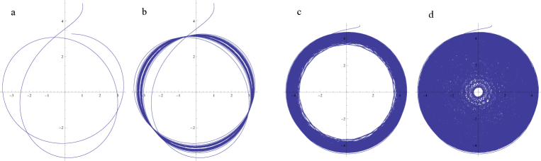
Figure 2. The trajectory of the ball on the plane with velocity $\Omega(t)=t$ for $0\leq t\leq 5$ and $0\leq t\leq 30.$ In the last two figures the velocity is changed $\Omega(t)=10t$ for $0\leq t\leq 20$ and $0\leq t\leq 30$

4.3. A example of a nonholonomic mechanical system with linear external forces: the vertical rolling disk with external forces

We will use the classical example of the vertical rolling disk to show how external forces can be encoded in the geometric structure of the constraint submanifold. Then, we are going to find the Hamilton-Jacobi equation and we obtain some particular solutions.

Consider a vertical disk that is allowed to roll on the $xy$-plane and to rotate about its vertical axis. Let $x,y$ denote the position of contact of the disk with the $xy$-plane, $\theta$ will denote the rotation angle of a chosen point $P$ of the disk with respect to the vertical axis and finally $\phi$ will represent the orientation angle of the disk as in Figure 3.

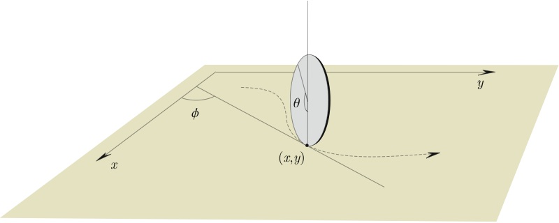
Figure 3. The vertical rolling disk

Therefore, the configuration space for the rolling disk is $Q=\mathbb{R}^{2}\times S^{1}\times S^{1}$ with coordinates $(x,y,\theta,\phi)$. On the tangent bundle $TQ\rightarrow Q$ we consider the Lie algebroid structure $([\cdot,\cdot]_{TQ},id_{TQ})$ where $[\cdot,\cdot]_{TQ}$ is the usual Lie bracket of vector fields and the anchor map, in this case, is $id_{TQ}$.

The Lagrangian for this system is:

$$L(x,y,\theta,\phi;\dot{x},\dot{y},\dot{\theta},\dot{\phi})=\frac{1}{2}\left(m(\dot{x}^{2}+\dot{y}^{2})+I\dot{\theta}^{2}+J\dot{\phi}^{2}\right)$$

where $m$ is the mass of the disk, $I$ its moment of inertia about the axis perpendicular to the plane containing the disk and $J$ is the moment of inertia about an axis in the plane of the disk. This Lagrangian induces a fiber metric

$$\mathcal{G}=m(dx\otimes dx+dy\otimes dy)+Id\theta\otimes d\theta+Jd\phi\otimes d\phi.$$

The nonholonomic constraints of rolling without slipping are

$$\left\{\begin{array}[]{l}\dot{x}=(R\cos\phi)\dot{\theta}\\ \dot{y}=(R\sin\phi)\dot{\theta}\end{array}\right.$$

and they define the constraint subbundle $\tau_{D}:D\rightarrow Q$ of $TQ$.

In terms of the fiber metric $\mathcal{G}$, we find an adapted basis for the nonholonomic problem. More precisely, we look for an orthonormal basis of vector fields $\{X_{1},X_{2},X_{3},X_{4}\}$ of $TQ$ such that $D=span\{X_{1},X_{2}\}$ and $D^{\perp}=span\{X_{3},X_{4}\}$. This basis is given by

$$X_{1} = \frac{1}{\sqrt{R^{2}m+I}}\left(R\cos\phi\frac{\partial}{\partial x}+R\sin\phi\frac{\partial}{\partial y}+\frac{\partial}{\partial\theta}\right)$$

$$X_{2} = \frac{1}{\sqrt{J}}\frac{\partial}{\partial\phi}$$

$$X_{3} = \frac{1}{\sqrt{m}}\left(\sin\phi\frac{\partial}{\partial x}-\cos\phi\frac{\partial}{\partial y}\right)$$

$$X_{4} = \sqrt{\frac{I}{m(R^{2}m+I)}}\left(\cos\phi\frac{\partial}{\partial x}+\sin\phi\frac{\partial}{\partial y}-\frac{Rm}{I}\frac{\partial}{\partial\theta}\right).$$

We endow the fiber bundle $\tau_{D}:D\rightarrow Q$ with a skew-symmetric algebroid structure $([\![\cdot,\cdot]\!]_{D},\rho_{D})$ defined by (see Example 2.6)

$$[\![X_{1},X_{2}]\!]_{D}=P([X_{1},X_{2}]_{TQ})\quad\mbox{and}\quad\rho_{D}(X_{1})=X_{1},\ \rho_{D}(X_{2})=X_{2},$$

where $P:TQ\rightarrow D$ is the orthogonal projector (with respect to the decomposition $TQ=D\oplus D^{\perp}$). Note that, $\rho_{D}=\rho_{TQ}\circ i_{D}$ with $i_{D}:D\hookrightarrow TQ$ the natural inclusion. Therefore, in terms of the basis $\{X_{1},X_{2}\}$, the (non zero) local structure functions of the skew-symmetric algebroid on $D$ are given by

$$(\rho_{D})_{1}^{x}=\frac{R\cos\phi}{\sqrt{mR^{2}+I}}, \ \ (\rho_{D})_{1}^{\theta}=\frac{1}{\sqrt{mR^{2}+I}},$$

$$(\rho_{D})_{1}^{y}=\frac{R\sin\phi}{\sqrt{mR^{2}+I}}, \ \ (\rho_{D})_{2}^{\phi}=\frac{1}{\sqrt{J}}.$$ (4.6)

Since $[X_{1},X_{2}]_{TQ}\in span\{X_{3}\}$ we have that $\mathcal{C}_{12}^{1}=\mathcal{C}_{12}^{2}=0$.

In coordinates  $(v^{1},v^{2},v^{3},v^{4})$  induced by the orthonormal basis of sections  $\{X_{1},X_{2},X_{3},X_{4}\}$  the Lagrangian is

$$L(x,y,\theta,\phi;v^{1},v^{2},v^{3},v^{4})=\frac{1}{2}\left((v^{1})^{2}+(v^{2})^{2}+(v^{3})^{2}+(v^{4})^{2}\right),$$

and the equations determining the constraints are $v^{3}=v^{4}=0$. Therefore, the restricted lagrangian $L_{D}:D\rightarrow\mathbb{R}$ becomes $L_{D}(x,y,\theta,\phi;v^{1},v^{2})=\frac{1}{2}\left((v^{1})^{2}+(v^{2})^{2}\right)$.

Consider now, the dual vector bundle  $\tau_{D^{*}}:D^{*}\rightarrow Q$    with coordinates  $(x,y,\theta,\phi;p_{1},p_{2})$ induced by the dual basis $\{X^{1},X^{2}\}$ of $\{X_{1},X_{2}\}$. Then, the vector bundle $\tau_{D^{*}}:D^{*}\rightarrow Q$ has a linear almost Poisson structure given by

$$\{x,p_{1}\}_{D^{*}}=\frac{R\cos\phi}{\sqrt{mR^{2}+I}}, \ \ \{\theta,p_{1}\}_{D^{*}}=\frac{1}{\sqrt{mR^{2}+I}},$$

$$\{y,p_{1}\}_{D^{*}}=\frac{R\sin\phi}{\sqrt{mR^{2}+I}}, \ \ \{\phi,p_{2}\}_{D^{*}}=\frac{1}{\sqrt{J}}$$

and the other fundamental brackets are zero.

In these coordinates, the Hamiltonian function $H:D^{*}\rightarrow\mathbb{R}$ can be written as

$$H(x,y,\theta,\phi;p_{1},p_{2})=\frac{1}{2}\left((p_{1})^{2}+(p_{1})^{2}\right).$$

It is very interesting the study of the rolling disk with external forces [35]. The system has two natural inputs, a torque that makes the disk spin and another one that makes the disk roll. First we are going to study the most general situation and then we will analyze particular cases. Suppose that a linear force is acting on the disk, then the pull back of this force in $D^{*}$ is given by $\tilde{F}(q,v)=(\tilde{F}_{1}^{1}(q)v^{1}+\tilde{F}_{2}^{1}(q)v^{2})X^{1}(q)+(\tilde{F}^{2}_{1}(q)v^{1}+\tilde{F}_{2}^{2}(q)v^{2})X^{2}(q),$ where $(q,v)=(x,y,\theta,\phi;v^{1},v^{2})$ and $F_{i}^{j}\in C^{\infty}(Q)$.

Since the chosen basis is orthonormal, we have that the homomorphism $F:D\rightarrow D$ induced by the force $\tilde{F}$ is

$$F(X_{1}) = \tilde{F}_{1}^{1}X_{1}+\tilde{F}_{1}^{2}X_{2}$$

$$F(X_{2}) = \tilde{F}_{2}^{1}X_{1}+\tilde{F}_{2}^{2}X_{2}$$

and thus the skew-symmetric algebroid on $\mathbb{R}\times D$ has (non zero) local structure functions given by $\mathcal{C}_{01}^{1}=-\tilde{F}_{1}^{1},\mathcal{C}_{01}^{2}=-\tilde{F}_{1}^{2},\mathcal{C}_{02}^{1}=-\tilde{F}_{2}^{1},\mathcal{C}_{02}^{2}=-\tilde{F}_{2}^{2}$ and equation (4.6).

Therefore, the corresponding Hamilton equations modified by the action of an external force are

$$\dot{x}=\frac{R\cos\phi}{\sqrt{I+mR^{2}}}p_{1},\ \ \ \dot{y}=\frac{R\sin\phi}{\sqrt{I+mR^{2}}}p_{1},$$

$$\dot{\theta}=\frac{1}{\sqrt{I+mR^{2}}}p_{1},\ \ \ \dot{\phi}=\frac{1}{\sqrt{J}}p_{2},$$

$$\dot{p}_{1}=-\tilde{F}_{1}^{1}p_{1}-\tilde{F}_{1}^{2}p_{2}\ \ \ \dot{p}_{2}=-\tilde{F}_{2}^{1}p_{1}-\tilde{F}_{2}^{2}p_{2}.$$

In order to write the Hamilton-Jacobi equations, let us consider a section $\alpha\in\Gamma(D^{*})$.

Then, such equations are

$$\begin{array}[]{rcl}\alpha_{1}.X_{1}(\alpha_{1})+\alpha_{2}.X_{1}(\alpha_{2})+\alpha_{2}.X_{2}(\alpha_{1})-\alpha_{2}.X_{1}(\alpha_{2})+\alpha_{1}.\tilde{F}_{1}^{1}+\alpha_{2}.\tilde{F}_{1}^{2}&=&0\\ \alpha_{1}.X_{2}(\alpha_{1})+\alpha_{2}.X_{2}(\alpha_{2})-\alpha_{1}.X_{2}(\alpha_{1})+\alpha_{1}.X_{1}(\alpha_{2})+\alpha_{1}.\tilde{F}_{2}^{1}+\alpha_{2}.\tilde{F}_{2}^{2}&=&0\end{array}$$ (4.7)

where $\alpha=\alpha_{1}X^{1}+\alpha_{2}X^{2}$ and $\alpha_{1},\alpha_{2}\in C^{\infty}(Q)$.

Particular case: A torque that makes the disk spin.

Let us consider the external force $\tilde{F}=\lambda(\phi)\dot{\phi}\,d\phi,$ with $\lambda\in C^{\infty}(\mathbb{R})$. Writing this force in terms of the dual basis $\{X^{1},X^{2}\}$ we obtain

$$\tilde{F}(q,v)=\frac{\lambda(\phi)}{{J}}v^{2}X^{2},$$

where $(q,v)=(x,y,\theta,\phi,v^{1},v^{2}).$ Therefore, the homomorphism $F:D\rightarrow D$ is

$$F(X_{1})=0\quad\mbox{and}\quad F(X_{2})=\frac{\lambda(\phi)}{{J}}X_{2}$$

and the skew-symmetric algebroid on $\mathbb{R}\times D$ has (non zero) local structure functions given by $\mathcal{C}_{02}^{2}=-\frac{\lambda(\phi)}{J}$ and (4.6).

Consider a section $\alpha\in\Gamma(D^{*})$ such that $\alpha=kX^{1}+\alpha_{2}(\phi)X^{2}$, with $k=constant.$

Thus, Hamilton-Jacobi equation (4.7) is simply (note that, in this case, $d^{E}\alpha=0$),

$$\alpha_{2}^{\prime}(\phi)=-\frac{\lambda(\phi)}{\sqrt{J}}.$$ (4.8)

Therefore, from (4.8), we deduce that

$$\alpha_{2}(\phi)=-\frac{1}{\sqrt{J}}\int_{0}^{\phi}\lambda(s)ds+\kappa$$

where $\kappa$ is an arbitrary constant.

By Eq. (3.1), we have

$$R_{h}^{\alpha}=\frac{R\,k\cos\phi}{\sqrt{I+mR^{2}}}\frac{\partial}{\partial x}+\frac{R\,k\sin\phi}{\sqrt{I+mR^{2}}}\frac{\partial}{\partial y}+\frac{k}{\sqrt{I+mR^{2}}}\frac{\partial}{\partial\theta}-\frac{1}{{J}}\left(\int_{0}^{\phi}\lambda(s)ds-\kappa\right)\frac{\partial}{\partial\phi}.$$

We conclude, by Corollary 4.1, that

$$\alpha\circ c(t)=(x(t),y(t),\theta(t),\phi(t);k,-\frac{1}{\sqrt{J}}\int_{0}^{\phi(t)}\lambda(s)ds-\kappa)$$

is an integral curve of $R_{h}\in{\mathfrak{X}}(D^{*})$, if $c(t)=(x(t),y(t),\theta(t),\phi(t))$ is an integral curve of $R_{h}^{\alpha}$.

As a particular case, we fix $\lambda(\phi)=K\cos\phi$ with $K=cte\neq 0$. Hence by equation (4.8) we have that $\alpha_{2}(\phi)=-\frac{K}{\sqrt{J}}\sin\phi+\kappa$ but, just for simplicity, we will choose $\kappa=0$. If $c:I\to Q$, $c(t)=(x(t),y(t),z(t),\theta(t),\phi(t))$, is an integral curve of $R_{h}^{\alpha}$ then $\dot{\phi}(t)=-\displaystyle\frac{K}{{J}}\sin\phi$. That is,

$$\phi(t)=2\arctan\left(e^{-\frac{K}{J}t+\phi_{0}}\right)$$

with $\phi_{0}$ an arbitrary constant. Therefore, the solution of the system, modified by an external force $\tilde{F}=(K\cos\phi)\dot{\phi}\,d\phi$ that makes the disk spin, is

$$\alpha\circ c(t)=(x(t),y(t),\theta(t),\phi(t);k,-\frac{K}{\sqrt{J}}\sin\phi(t)),$$

where $x(t),y(t),\theta(t),\phi(t)$ are curves given by

$$x(t) = \frac{R\,k}{\sqrt{I+mR^{2}}}\left(t+\frac{J}{K}\ln\left(1+e^{-2\frac{K}{J}t+2\phi_{0}}\right)\right)+x_{0}$$

$$y(t) = \frac{J}{K}\frac{R\,k}{\sqrt{I+mR^{2}}}\phi(t)+y_{0}$$

$$\theta(t) = \frac{kt}{\sqrt{I+mR^{2}}}+\theta_{0}$$

$$\phi(t) = 2\arctan\left(e^{-\frac{K}{J}t+\phi_{0}}\right)$$

where $x_{0},y_{0},\theta_{0},\phi_{0}$ are arbitrary constants.

We also have the dissipative term for this case given by

$$\{H\circ\mu,F_{h}\}=-\frac{K\cos\phi}{J}(p_{2})^{2}.$$

Remark 4.13.

The function $f\in C^{\infty}(Q)$, given by

$$f(\phi)=\frac{-1}{2J}\left(\int_{0}^{\phi}\lambda(s)ds\right)^{2}=-\frac{K^{2}}{2J}\sin^{2}\phi$$

verifies that $F^{*}\alpha=d^{D}f$. Thus, we obtain that the Hamilton Jacobi equation can be written as

$$H\circ\alpha-\frac{K^{2}}{2J}\sin^{2}\phi=constant,$$

on $Q$, since $D$ is a completely nonholonomic distribution. $\diamond$

5. Conclusions and future work

A Hamilton-Jacobi equation for a great variety of mechanical systems is derived. The type of systems considered includes mechanical systems with dissipative forces, nonholonomic system subjected to linear or affine constraints or, even, explicitly time-dependent mechanical systems. With this general purpose in mind, we find that the geometric structure of skew-symmetric algebroid has the appropriate inclusive nature, adequate to model all these different types of mechanical systems. Adopting this point of view we prove a general version of the Hamilton-Jacobi equation for skew-symmetric algebroids with a distinguished cocycle, specializing the results for the different mechanical systems under study. Several examples prove the utility and novelty of our results.

Of course, a lot of work must be done in future research. For instance, in our paper a crucial assumption is made: all the constraints are linear or affine, even the dissipative forces considered are of a very special type (in such a way that they induce a linear bivector on the dual bundle). It would be interesting to discuss the more general case in a non-linear setting, discovering the underlying geometric structures and deriving, if possible, a Hamilton-Jacobi equation. Moreover, in future papers, we will study more explicit examples of applications of our theoretical setting, analyzing when the separation of variables technique works and relating it with topics like integrability. Also, our setting is ready for the introduction of control forces and therefore for the study of controlled mechanical systems and, as a consequence, to address problems like kinematic reduction, kinematic controllability, Hamilton-Jacobi-Bellman equation in optimal control, etc.

References

- [1] R. Abraham, J.E. Marsden: Foundations of Mechanics, Second Edition, Benjamin, New York, 1978.
- [2] A.A. Agrachev, Y. Sachkov: Control theory from the geometric view-point, Encyclopedia of Mathematical Science, Vol 87. Control theory and optimization. Springer-Verlag, Berlin (2004)
- [3] P. Balseiro, M. de León, J.C. Marrero, D. Martín de Diego: The ubiquity of the symplectic hamiltonian equations in mechanics, J. Geometric Mechanics, 1 (2009) 1-34.
- [4] F. Cantrijn, M. de León, J.C. Marrero, D. Martín de Diego: On almost-Poisson structures in non-holonomic mechanics II. The time dependent framework. Nonlinearity, 13 (2000), 1379-1409.
- [5] F. Cantrijn, M. de León, D. Martín de Diego: On almost-Poisson structures in non-holonomic mechanics; Nonlinearity, 12 (1999), 721-737.
- [6] J. F. Cariñena, X. Gracia, G. Marmo, E. Martínez, M. C. Muñoz-Lecanda, N. Roman–Roy : Geometric Hamilton-Jacobi Theory for Nonholonomic Dynamical Systems, Preprint (2009) arXiv:0908.2453.
- [7] J. Cortés, M. de León, J.C. Marrero, D. Martín de Diego, E. Martínez: A survey of Lagrangian mechanics and control on Lie algebroids and groupoids, Int. J. Geom. Methods Mod. Phys. 3 (2006), no. 3, 509–558.
- [8] J. Cortés, M. de León, J.C. Marrero, E. Martínez: Nonholonomic Lagrangian systems on Lie algebroids, Discrete and Continuous Dynamical Systems: Series A, 24 (2) (2009), 213–271.
- [9] J. Cortés, E. Martínez: Mechanical control systems on Lie algebroids, IMA J. Math. Control. Inform. 21 (2004), 457–492.
- [10] K. Grabowska, J. Grabowski: Variational calculus with constriants on general algebroids, J. Phys. A: Math Theoret., 41 (2008), 175204.
- [11] K. Grabowska, J. Grabowski, P. Urbański: AV-differential Geometry: Poisson and Jacobi structures, Journal of Geometry and Physics, 52 (2004) 398–446.
- [12] K. Grabowska, J. Grabowski, P. Urbański: Geometrical mechanics on algebroids, Int. J. Geom. Methods Mod. Phys. 3 (3) (2006), 559575.
- [13] J. Grabowski, M. de León, J.C. Marrero, D. Martín de Diego: Nonholonomic constraints: a new viewpoint, J. Math. Phys. 50 (2009), no. 1, 013520, (17 pp)
- [14] J. Grabowski, P. Urbański: Lie algebroids and Poisson-Nijenhuis structures, Rep. Math. Phys. 40 (1997), 195–208.
- [15] J. Grabowski, P. Urbański: Algebroids general differential calculi on vector bundles, J. Geom. Phys. 31 (1999), 111–141.
- [16] A. Ibort, M. de León, J. C. Marrero, D. Martín de Diego: Dirac brackets in constrained dynamics, Fortschr. Phys., 47 (1999), 459–492
- [17] D. Iglesias, M. de León, D. Martín de Diego: Towards a Hamilton-Jacobi Theory for Nonholonomic Mechanical Systems, J. Phys. A: Math. Theor. 41 (2008) 015205 (14pp).
- [18] D. Iglesias, J.C. Marrero, D. Martín de Diego, D. Sosa: A general framework for nonholonomic mechanics: Nonholonomic systems on Lie affgebroids, J. Math. Phys., 48 (2007) 083513.
- [19] D. Iglesias, J.C. Marrero, E. Padrón, D. Sosa: Lagrangian submanifolds and dynamics on Lie affgebroids, Rep. Math. Phys. 38 (2006) 385–436.
- [20] W.S. Koon, J.E. Marsden: Poisson reduction of nonholonomic mechanical systems with symmetry, Rep. Math. Phys. 42 (1/2) (1998), 101–134.
- [21] R. Krechetnikov, J. E. Marsden: Dissipation-induced instabilities in finite dimensions, Reviews of Modern Physics, 79 (2), (2007), 519–553.
- [22] M. de León, J.C. Marrero, D. Martín de Diego: Linear almost Poisson structures and Hamilton-Jacobi theory. Applications to nonholonomic Mechanics, Preprint 2008, arXiv:0801.4358.
- [23] M. de León, J.C. Marrero, E. Martínez: Lagrangian submanifolds and dynamics on Lie algebroids, J. Phys. A: Math. Gen. 38 (2005), R241–R308.
- [24] M. de León, P.R. Rodrigues: Methods of Differential Geometry in Analytical Mechanics, North Holland Math. Series 152 (Amsterdam, 1996).
- [25] P. Libermann: Lie algebroids and Mechanics, Arch. Math. (Brno), 32 (1996), 147-162.
- [26] K. Mackenzie: General Theory of Lie groupoids and Lie algebroids in differential geometry, London Mathematical Society Lecture Note Series, No. 124, 2005.
- [27] J.C. Marrero, D. Martín de Diego, D. Sosa: Variational constrained Mechanics on Lie affgebroids, Discrete and Continuous dynamical Systems, Series S, 3, (1) (2010) 105-128.
- [28] J.C. Marrero, D. Sosa: The Hamilton-Jacobi equation on Lie affgebroids, Int. J. Geom. Meth. Mod. Phys. 3 (3) (2006) 605–622.
- [29] E. Martínez: Lagrangian mechanics on Lie algebroids, Acta Appl. Math. 67 (2001), no. 3, 295–320.
- [30] E. Martínez, T. Mestdag, W. Sarlet: Lie algebroid structures and Lagrangian systems on affine bundles. J. Geom. Phys. 44 (2002), no. 1, 70–95.
- [31] T. Mestdag: Lagrangian reduction by stages for nonholonomic systems in a Lie algebroid framework, J. Phys. A: Math. Gen. 38 (2005), 10157–10179.
- [32] T. Mestdag, B. Langerock: A Lie algebroid framework for nonholonomic systems, J. Phys. A: Math. Gen 38 (2005), 1097–1111.
- [33] R. Montgomery: A Tour of Subriemannian Geometries, their geodesics and applicaions. Mathematical Surveys and Monographs, 91. AMS. 2002.
- [34] C.D. Murray: Dynamical effects of drag in the circular restricted three-body problem, Icarus 112 (1994), 465-484.
- [35] A.D. Lewis: Simple Mechanical Control Systems with Constraints. IEE Transactions on Automatic Control, 45 (8), (2000), 1420-1436.
- [36] T. Ohsawa, A.M. Bloch: Nonholonomic Hamilton-Jacobi equation and Integrability, Preprint 2009, arXiv:0906.3357.
- [37] M. Popescu, P. Popescu: Geometric objects defined by almost Lie structures, Proc. Workshop on Lie algebroids and related topics in Differential Geometry (Warsaw) 54 (Warsaw: Banach Center Publications) (2001), 217—233.
- [38] D. Sosa: Afgebroides de Lie y Mecánica Geométrica, Dissertation Thesis, available in http://www.gmcnetwork.org/files/thesis/dsosa.pdf
- [39] H.J. Sussmann: Orbits of families of vector fields and integrability of distributions, Transactions of the American Mathematical Society, 180, (1973), 171 188.
- [40] A.J. Van Der Schaft, B. M. Maschke: On the Hamiltonian formulation of non-holonomic mechanics systems, Rep. Math. Phys., 34 (1994), 225–233.
- [41] A. Weinstein: Lagrangian Mechanics and Groupoids, in “Mechanics day” (Waterloo, ON, 1992), Fields Institute Communications 7, American Mathematical Society, (1996), 207–231.