Response functions of cold neutron matter: density fluctuations

Abstract

We compute the finite temperature density response function of nonrelativistic cold fermions with an isotropic condensate. The pair-breaking contribution to the response function evaluated in the limit of small three-momentum transfers $q$ within an effective theory which exploits series expansion in powers of small $q/p_{F}$, where $p_{F}$ is the Fermi momentum. The leading order $O(q^{2})$ contribution is universal and depends only on two fundamental scales, the Fermi energy and the pairing gap. The particle-hole Landau Fermi-liquid interaction contributes first at the next-to-leading order $O(q^{4})$. The scattering contribution to the polarization tensor is nonperturbative (in the above sense) and is evaluated numerically. The spectral functions of density fluctuations are constructed and the relevance of the $q^{2}$ scaling for the pair breaking neutrino emission from neutron stars is discussed.

I Introduction

The long-wavelength, low-energy dynamics of fermionic systems is determined by their response functions to soft perturbations, which are characterized by length scales that are large compared to the inverse Fermi wave vector and energies that are small compared to the Fermi energy. At zero temperature the response functions of pair-correlated nuclear matter have been studied long ago by Larkin and Migdal Migdal_book . Recently, the response functions of pair-correlated nuclear systems at nonzero temperature received attention in the context of neutral current neutrino emission via pair breaking and formation in compact stars Sedrakian:2006ys ; Kolomeitsev:2008mc ; Steiner:2008qz ; Leinson:2009mq and neutrino scattering in supernovae Kundu:2004mz . The evaluation of the response functions involves typically a resummation of infinite number of finite temperature ring diagrams. In the unpaired limit of normal Fermi liquid, this resummation scheme reduced to the familiar random-phase-approximation (RPA); for recent applications in nucleonic and neutron star matter, see Refs. Olsson:2004ea ; Lykasov:2005xh ; Margueron:2005nc ; Baldo:2008pb .

In attractive, cold, fermionic systems the gap $\Delta$ in the quasiparticle spectrum is small compared to the Fermi energy and the hierarchy of energy scales depends on the magnitude of the perturbation, which can take arbitrary values with respect to the pairing gap $\Delta$. In this work we focus on density perturbations and show that the two distinct contributions to the response function through the scattering and pair breaking processes are effective below and above the energy threshold $2\Delta$, i.e., the energy needed to break a pair. The pair breaking processes are of special importance for applications in compact stars; to evaluate them, we propose a new systematic low-transferred-momentum expansion of the response function which builds on the previous work on polarization tensors of cold superfluid fermionic systems Sedrakian:2006ys . Specifically, we show that the pair breaking contribution to the polarization tensor posses a well-defined expansion with respect to the ratio of the momentum of the external current to the Fermi momentum of the fermions. We also adopt more general ansatz for the driving terms in the integral equations of Ref. Sedrakian:2006ys by lifting the degeneracy among the particle-particle and particle-hole channels. We work in the nonrelativistic limit, i.e., the ratio of the Fermi velocity to the speed of light is small ($v_{F}/c\ll 1$).

The density response functions can be utilized to determine the spectrum of the collective modes, the stability of the system toward clustering, the rates of electromagnetic and weak radiation processes, and so on. In particular, the rates of neutrino reactions in stellar interiors can be expressed through the response function of underlying matter to vector and axial-vector weak currents Burrows:1998ek ; Sedrakian:1999jh ; Sedrakian:2000kc ; Sedrakian:2006mq . In nonrelativistic limit, the vector and axial-vector responses are mapped onto the responses to the density and spin-density perturbations, respectively. The response functions in the superfluid neutron matter were recently computed and the neutrino emission rates were determined in Refs. Sedrakian:2006ys ; Kolomeitsev:2008mc ; Steiner:2008qz ; Leinson:2009mq . Phenomenologically, these are important in modeling the cooling of intermediate age neutron stars and the superburst in accreting neutron stars Brown:2009kw ; Page:2009fu ; Gupta:2006fd .

It is now well established that at zeroth order ($\bm{q}=0$) the pair breaking density response function vanishes, as required by the $f$-sum rule for the polarization tensor, which is a direct consequence of the baryon number conservation. Some authors found analytically the leading-order contribution to the polarization which arises at order $q^{4}$ Leinson:2006gf ; Kolomeitsev:2008mc . Since there is no general argument that requires the coefficient of the leading-order $q^{2}$ term to be zero, the answer may depend on the approximations involved in the theory. In section III.1 we study in detail a new small $q$ expansion of the polarization tensor obtained in Ref. Sedrakian:2006ys and find that the coefficient of the $q^{2}$ term in the series expansion of the density response function is indeed nonzero. Furthermore, it turns out to be universal, i.e., it depends only on two fundamental scales of the problem, the Fermi energy and pairing gap, and is independent of the strength of particle-hole interaction.

This paper is organized as follows. In Sec. II we derive the vertex functions and polarization tensor in a more general setting that in Ref. Sedrakian:2006ys by using different particle-particle and particle-hole interactions and clarify the approximations that arise in the weak coupling Bardeen-Cooper-Schrieffer (BCS) limit. A small momentum transfer expansion is applied to the pair breaking polarization tensor in Sec. III.1. We also show in Sec. III.2 the results of exact numerical evaluation of the scattering part of the polarization tensor. Further in Sec. III.3 we verify that the unpaired and uncorrelated limits are recovered from the scattering part. Our conclusions are collected in Sec. IV. Details of calculations are presented in Appendices A and B. We use the natural units $\hbar=c=1$ throughout and assume that the Boltzmann constant $k_{B}=1$.

II Density response function

In this section we derive the general form of the density-response function of neutron matter at nonzero temperature. At densities below the saturation density neutron matter forms a ${}^{1}S_{0}$ pair condensate and can be described by the weak coupling limit of the BCS theory. This affects not only the approximations that are applied to the gap equation, but also the approximate relations between the loop integrals, as we discuss below.

The couplings in the particle-particle ($pp$) and particle-hole ($ph$) channels, $v_{pp}$ and $v_{ph}$, are assumed zero range; often their values are taken to be degenerate $v_{pp}=v_{ph}$ and equal to the lowest order Landau parameter $f_{0}$. We shall lift this approximation below by assuming $v_{pp}\neq v_{ph}$. The spectrum of paired neutrons is given by

$$\epsilon_{p}=\sqrt{\xi_{p}^{2}+\Delta^{2}(\bm{p})},$$ (1)

where $\xi_{p}=p^{2}/2m^{*}-\mu$ is the quasiparticle spectrum in the normal state, $\Delta(\bm{p})$ is the energy gap, $\bm{p}$ is the three-momentum, $m^{*}$ is the effective mass and $\mu$ is the chemical potential. For contact pairing interaction the gap is momentum independent, $\Delta(\bm{p})\equiv\Delta$.

The softness of the modes implies that their wave vector $|\bm{q}|\ll p_{F}$. Accordingly, we write

$$\xi_{p+q}=\frac{p^{2}}{2m^{*}}\left(1+\frac{2\bm{p}\cdot\bm{q}}{p^{2}}+\frac{q^{2}}{p^{2}}\right)-\mu,$$ (2)

and consider the second and third terms in the bracket as small compared to unity, since $p\simeq p_{F}$, where $p_{F}$ is the Fermi momentum. Thus, we may write $\xi_{p+q}\simeq\xi_{p}+\mu_{0}(2yx+y^{2})$, where $x=(\bm{p}\cdot\bm{q})/(|p||q|)$ and $y={q}/{p_{F}}$, whereby $y\ll 1$. Here $\mu_{0}=p_{F}^{2}/2m^{*}$ is the chemical potential at zero temperature; we shall drop the 0 index in the following. Several observations are in order:

1. If the expansion is carried out with respect to the small parameter $\delta\xi=\xi_{p+q}-\xi_{p}$, as in Ref. Sedrakian:2006ys , the power counting is not manifest. At the leading-order the terms which scale linearly in $x$ drop on angle integration in symmetrical limits. The only nonzero contribution proportional to $q^{2}$ is then furnished by the recoil term. One needs to carry out the $\delta\xi$ expansion at least to second order to obtain all relevant terms that are of order $q^{2}$.

2. An alternative to the expansion with respect to $\delta\xi$ is the expansion with respect to the ratio $y=|\bm{q}|/p_{F}$. This expansion exploits the softness of the modes and applies both for timelike and spacelike momentum transfers. It is an alternative to expansions in the ratios $\omega/qv_{F}$ and $qv_{F}/\omega$, which are valid in these regimes, respectively.

3. Organizing the expansion in powers of $v_{F}/c\ll 1$ (nonrelativistic fermions) does not guarantee per se the convergence of the series. At any fixed density, the Fermi velocity $v_{F}$ is constant and for sufficiently large momentum transfers ($q\geq p_{F}/2$) the series will fail to converge.

4. Finally, the smallness of the expansion parameter is necessary but not sufficient condition for the convergence of the Taylor series. The validity of the expansion should be checked by an exact numerical computation of the loop integrals.

In the following we shall demonstrate that the pair breaking part of the response function can be expanded systematically with respect to the $y$ parameter. Such expansion is thus valid for small three-momentum transfers, but arbitrary energy transfers.

II.1 Vertex functions

We start with integral equations for the vertex functions and derive a (slight) generalization of their counterparts in Ref. Sedrakian:2006ys that distinguish the particle-particle and particle-hole interactions. These we write as sums of central and spin-spin interaction terms

$$V^{pp} \simeq v_{pp}+v_{pp}({\bm{\sigma}}\cdot{\bm{\sigma}}^{\prime})+\dots,$$ (3)

$$V^{ph} \simeq v_{ph}+v_{ph}({\bm{\sigma}}\cdot{\bm{\sigma}}^{\prime})+\dots,$$ (4)

where the ellipses stand for the tensor and spin-orbit terms that are subdominant at relevant densities in neutron matter.

The integral equations defining the scalar vertex, which we write in an operator form, are given by Migdal_book ; Sedrakian:2006ys

$$\hat{\Gamma}_{1} = \Gamma_{0}+v_{ph}(G\Gamma_{1}G+\hat{F}\hat{\Gamma}_{3}G+G\hat{\Gamma}_{2}\hat{F}+\hat{F}\Gamma_{4}\hat{F}),$$ (5)

$$\hat{\Gamma}_{2} = \quad\quad v_{pp}(G\hat{\Gamma}_{2}G^{\dagger}+\hat{F}\Gamma_{4}G^{\dagger}+G\Gamma_{1}\hat{F}+\hat{F}\hat{\Gamma}_{3}\hat{F}),$$ (6)

$$\hat{\Gamma}_{3} = \quad\quad v_{pp}(G^{\dagger}\hat{\Gamma}_{3}G+\hat{F}\Gamma_{1}G+G^{\dagger}\Gamma_{4}\hat{F}+\hat{F}\hat{\Gamma}_{2}\hat{F}),$$ (7)

$$\hat{\Gamma}_{4} = \Gamma_{0}+v_{ph}(G^{\dagger}\Gamma_{4}G^{\dagger}+\hat{F}\Gamma_{1}\hat{F}+\hat{F}\hat{\Gamma}_{2}G^{\dagger}+G^{\dagger}\hat{\Gamma}_{3}\hat{F}).$$

Here $\hat{F}=-i\sigma_{y}F$, $\sigma_{y}$ is the second component of the Pauli matrix, $\Gamma_{0}=1$. When $v_{pp}=v_{ph}$, Eqs. (5)-(II.1) become identical to those of Ref. Sedrakian:2006ys . Let us now define the “elementary loop” as

$$\Pi_{XX^{\prime}}(q)=g\int\frac{d^{4}p}{(2\pi)^{4}}X(p)X^{\prime}(p+q),$$ (9)

where $X\in\{G,G^{\dagger},F,F^{\dagger}\}$ and $g$ is the degeneracy factor, which we omit in the intermediate equations and restore in the final ones. Direct calculations show that

$$\Pi_{G^{\dagger}F}=\Pi_{FG},\quad\Pi_{GF}=\Pi_{FG^{\dagger}},\quad\Pi_{G^{\dagger}G^{\dagger}}=\Pi_{GG};$$ (10)

these equalities imply that $\Gamma_{1}=\Gamma_{4}$, which is a consequence of the time-reversal invariance of the system. The remaining equations read

$$\left(\begin{array}[]{ccc}1-v_{ph}[\Pi_{GG}-\Pi_{FF}]&v_{ph}\Pi_{GF}&v_{ph}\Pi_{FG}\\ -2v_{pp}\Pi_{GF}&[1-v_{pp}\Pi_{GG^{\dagger}}]&v_{pp}\Pi_{FF}\\ -2v_{pp}\Pi_{FG}&v_{pp}\Pi_{FF}&[1-v_{pp}\Pi_{G^{\dagger}G}]\end{array}\right)\left(\begin{array}[]{c}\Gamma_{1}\\ \Gamma_{2}\\ \Gamma_{3}\end{array}\right)=\left(\begin{array}[]{c}\Gamma_{0}\\ 0\\ 0\end{array}\right).$$ (11)

There are six distinct loops in Eq. (11), namely $\Pi_{GG}$, $\Pi_{FF}$, $\Pi_{GF}$, $\Pi_{FG}$, $\Pi_{G^{\dagger}G}$, $\Pi_{GG^{\dagger}}$. In the weak coupling limit $\Pi_{GF}\simeq-\Pi_{FG}$, $\Pi_{G^{\dagger}G}\simeq\Pi_{GG^{\dagger}}$, an approximation discussed in detail in Sec. II.2. This reduces the number of equations from three to two

$$\left(\begin{array}[]{ccc}1-v_{ph}{\cal A}&v_{ph}{\cal B}\\ -v_{pp}{\cal B}&-v_{pp}{\cal C}\\ \end{array}\right)\left(\begin{array}[]{c}\Gamma_{1}\\ \Gamma_{2}\\ \end{array}\right)=\left(\begin{array}[]{c}\Gamma_{0}\\ 0\end{array}\right),$$ (18)

where

$${\cal A}(q) = \Pi_{GG}(q)-\Pi_{FF}(q),$$ (19)

$${\cal B}(q) = 2\Pi_{FG}(q),$$ (20)

$${\cal C}(q) = \Pi_{GG^{\dagger}}(q)+\Pi_{FF}(q)-(v_{pp})^{-1},$$ (21)

with $q=(\omega,\bm{q})$. The solutions for the remaining two vertex functions reads

$$\Gamma_{1}(q) = \frac{\Gamma_{0}{\cal C}(q)}{{\cal C}(q)-v_{ph}[{\cal A}(q){\cal C}(q)+{\cal B}(q)^{2}]},$$ (22)

$$\Gamma_{2}(q) = -\frac{\Gamma_{0}{\cal B}(q)}{{\cal C}(q)-v_{ph}[{\cal A}(q){\cal C}(q)+{\cal B}(q)^{2}]}.$$ (23)

When $v_{pp}=v_{ph}$ these reduce to Eqs. (22) and (23) of Ref. Sedrakian:2006ys . It seen that the interaction in the $pp$ channel is absorbed in the gap equation and it is the $ph$ interaction that enters the renormalization of the one-loop polarization tensor. This result could have been anticipated from the limiting form of the RPA polarization tensor of normal Fermi liquids (see Sec. III.3).

II.2 Polarization tensor

The full polarization tensor is given by Eq. (35) of Ref. Sedrakian:2006ys with the replacement $v\to v_{ph}$

$$\Pi^{R}(q)=\frac{{\cal A}(q){\cal C}(q)+{\cal B}(q)^{2}}{{\cal C}(q)-v_{ph}[{\cal A}(q){\cal C}(q)+{\cal B}(q)^{2}]}.$$ (24)

The “elementary loops” are defined explicitly as

$$\Pi_{GG}(q) = \int\frac{d^{3}p}{(2\pi)^{3}}\Biggl{\{}\left[\frac{u_{p}^{2}u_{k}^{2}}{iq+\epsilon_{p}-\epsilon_{k}}-\frac{v_{p}^{2}v_{k}^{2}}{iq-\epsilon_{p}+\epsilon_{k}}\right]\left[f(\epsilon_{p})-f(\epsilon_{k})\right]$$ (25)

$$+ \left[\frac{u_{k}^{2}v_{p}^{2}}{iq-\epsilon_{p}-\epsilon_{k}}-\frac{u_{p}^{2}v_{k}^{2}}{iq+\epsilon_{p}+\epsilon_{k}}\right]\left[f(-\epsilon_{p})-f(\epsilon_{k})\right]\Biggr{\}},$$

$$\Pi_{FG}(q) = -\int\frac{d^{3}p}{(2\pi)^{3}}\Biggl{\{}u_{p}v_{p}\left[\frac{u_{k}^{2}}{iq+\epsilon_{p}-\epsilon_{k}}+\frac{v_{k}^{2}}{iq-\epsilon_{p}+\epsilon_{k}}\right]\left[f(\epsilon_{p})-f(\epsilon_{k})\right]$$ (26)

$$- u_{p}v_{p}\left[\frac{u_{k}^{2}}{iq-\epsilon_{p}-\epsilon_{k}}+\frac{v_{k}^{2}}{iq+\epsilon_{p}+\epsilon_{k}}\right]\left[f(-\epsilon_{p})-f(\epsilon_{k})\right]\Biggr{\}},$$

$$\Pi_{FF}(q) = \int\frac{d^{3}p}{(2\pi)^{3}}\Biggl{\{}u_{p}u_{k}v_{p}v_{k}\Biggl{\{}\left[\frac{1}{iq+\epsilon_{p}-\epsilon_{k}}-\frac{1}{iq-\epsilon_{p}+\epsilon_{k}}\right]\left[f(\epsilon_{p})-f(\epsilon_{k})\right]$$ (27)

$$+ \left[\frac{1}{iq+\epsilon_{p}+\epsilon_{k}}-\frac{1}{iq-\epsilon_{p}-\epsilon_{k}}\right]\left[f(-\epsilon_{p})-f(\epsilon_{k})\right]\Biggr{\}}\Biggr{\}},$$

$$\Pi_{G^{\dagger}G}(q) = -\int\frac{d^{3}p}{(2\pi)^{3}}\Biggl{\{}\left[\frac{u_{k}^{2}v_{p}^{2}}{iq+\epsilon_{p}-\epsilon_{k}}-\frac{u_{p}^{2}v_{k}^{2}}{iq-\epsilon_{p}+\epsilon_{k}}\right]\left[f(\epsilon_{p})-f(\epsilon_{k})\right]$$ (28)

$$+ \left[\frac{u_{p}^{2}u_{k}^{2}}{iq-\epsilon_{p}-\epsilon_{k}}-\frac{v_{p}^{2}v_{k}^{2}}{iq+\epsilon_{p}+\epsilon_{k}}\right]\left[f(-\epsilon_{p})-f(\epsilon_{k})\right]\Biggr{\}},$$

where $k=p+q$ and the coherence factors are given by $u_{p}^{2}=(1/2)[1+\xi_{p}/\epsilon_{p}]$ and $v_{p}^{2}=1-u_{p}^{2}$.

The expression for $\Pi_{FG}(q)$ above applies at arbitrary couplings; however Eq. (20) presumes weak-coupling approximation, because $\Pi_{GF}(q)=-\Pi_{FG}(q)$ holds only in this limit. The weak-coupling limit for the function $\Pi_{FG}(q)$ is obtained on substituting in square braces $u_{k}^{2}=u_{p}^{2}=v_{p}^{2}=v_{k}^{2}=1/2$. This statement is equivalent to ignoring integrals of the type

$$I = \int\frac{d^{3}p}{(2\pi)^{3}}\frac{\Delta^{2}}{2\epsilon_{p}}\frac{\xi_{p}}{\epsilon_{p}}\frac{f(\epsilon_{p})-f(\epsilon_{k})}{iq+\epsilon_{p}-\epsilon_{k}}\simeq 0.$$ (29)

The integral vanishes because $\xi_{p}$ changes sign for momenta above and below the Fermi momentum, while the remainder of the integrand is an even function in the vicinity of $p_{F}$. Thus the loop polarization function reduces to

$$\Pi_{FG}(q) = -\frac{1}{2}\int\frac{d^{3}p}{(2\pi)^{3}}\Biggl{\{}u_{p}v_{p}$$ (30)

$$\left[\frac{1}{iq+\epsilon_{p}-\epsilon_{k}}+\frac{1}{iq-\epsilon_{p}+\epsilon_{k}}\right]\left[f(\epsilon_{p})-f(\epsilon_{k})\right]$$

$$- u_{p}v_{p}\left[\frac{1}{iq-\epsilon_{p}-\epsilon_{k}}+\frac{1}{iq+\epsilon_{p}+\epsilon_{k}}\right]$$

$$\left[f(-\epsilon_{p})-f(\epsilon_{k})\right]\Biggr{\}}.$$

The form of the polarization loop $\Pi_{G^{\dagger}G}(q)$ is valid for arbitrary couplings. The relation $\Pi_{G^{\dagger}G}(q)=\Pi_{GG^{\dagger}}(q)$ is established on noting that, for example, $u_{p}^{2}v_{k}^{2}=(u_{p}^{2}v_{k}^{2}-u_{k}^{2}v_{p}^{2})+u_{k}^{2}v_{p}^{2}$ and that the combination in braces vanishes in the weak coupling as it leads to an integral of the type (29).

The contributions to the polarization function due to quasiparticle scattering and pair breaking separate. For the contributions from scattering the poles are located at $\pm(\epsilon_{p}-\epsilon_{k})$ and the distribution is given by the combination $f(\epsilon_{p})-f(\epsilon_{k})$. For the pair breaking contributions the poles are located at $\pm(\epsilon_{p}+\epsilon_{k})$ and the distribution is proportional $1-f(\epsilon_{p})-f(\epsilon_{k})$. The pair breaking contribution vanishes in the limit $T\to T_{c}^{-}$ ($T$ is the temperature, $T_{c}$ is the critical temperature of the phase transition).

Now we write the retarded polarization functions $\Pi^{R}(q)$ in terms of the functions ${\cal A}(q)$, ${\cal B}(q)$ and ${\cal C}(q)$ after performing analytical continuation ($iq\to\omega+i\delta$) in functions $\Pi_{GG}(q)$, $\Pi_{FF}(q)$, $\Pi_{FG}(q)$ $\Pi_{G^{\dagger}G}(q)$. After some straightforward algebraic transformations we find

$${\cal A}(q) = \int\frac{d^{3}p}{(2\pi)^{3}}\Biggl{\{}\frac{1}{2}(\epsilon_{k}-\epsilon_{p})\left[1+\frac{\xi_{p}\xi_{k}}{\epsilon_{p}\epsilon_{k}}-\frac{\Delta^{2}}{\epsilon_{p}\epsilon_{k}}\right]\frac{f(\epsilon_{p})-f(\epsilon_{k})}{(\omega+i\delta)^{2}-(\epsilon_{p}-\epsilon_{k})^{2}}$$ (31)

$$+ \frac{1}{2}(\epsilon_{p}+\epsilon_{k})\left[1-\frac{\xi_{p}\xi_{k}}{\epsilon_{p}\epsilon_{k}}+\frac{\Delta^{2}}{\epsilon_{p}\epsilon_{k}}\right]\frac{f(-\epsilon_{p})-f(\epsilon_{k})}{(\omega+i\delta)^{2}-(\epsilon_{p}+\epsilon_{k})^{2}}\Biggr{\}},$$

$${\cal B}(q) = -\Delta\omega\int\frac{d^{3}p}{(2\pi)^{3}}\frac{1}{\epsilon_{p}}\Biggl{[}\frac{f(\epsilon_{p})-f(\epsilon_{k})}{(\omega+i\delta)^{2}-(\epsilon_{p}-\epsilon_{k})^{2}}-\frac{f(-\epsilon_{p})-f(\epsilon_{k})}{(\omega+i\delta)^{2}-(\epsilon_{p}+\epsilon_{k})^{2}}\Biggr{]},$$ (32)

$${\cal C}(q) = \frac{1}{2}\int\frac{d^{3}p}{(2\pi)^{3}}\Biggl{\{}\left[(\epsilon_{p}-\epsilon_{k})\left(1-\frac{\xi_{p}\xi_{k}}{\epsilon_{p}\epsilon_{k}}-\frac{\Delta^{2}}{\epsilon_{p}\epsilon_{k}}\right)\right]\frac{f(\epsilon_{p})-f(\epsilon_{k})}{(\omega+i\delta)^{2}-(\epsilon_{p}-\epsilon_{k})^{2}}$$ (33)

$$- \left[(\epsilon_{p}+\epsilon_{k})\left(1+\frac{\xi_{p}\xi_{k}}{\epsilon_{p}\epsilon_{k}}+\frac{\Delta^{2}}{\epsilon_{p}\epsilon_{k}}\right)\right]\frac{f(-\epsilon_{p})-f(\epsilon_{k})}{(\omega+i\delta)^{2}-(\epsilon_{p}+\epsilon_{k})^{2}}-\frac{1}{\epsilon_{p}}\left[1-2f(\epsilon_{p})\right]\Biggr{\}}.$$

Note that $\lim_{\bm{q}\to 0,\omega\to 0}{\cal C}(q)=0$, since the coupling constant in the particle-particle channel can be expressed as

$$(v_{pp})^{-1} = \Pi_{G^{\dagger}G}(q=0)+\Pi_{FF}(q=0)$$ (34)

$$= \int\frac{d^{3}p}{(2\pi)^{3}}\frac{1}{2\epsilon_{p}}\left[1-2f(\epsilon_{p})\right],$$

which is the gap equation for the contact interaction $v_{pp}$. We do not need to specify the regularization of the gap equation, since its divergence is eliminated in the loop integrals. For numerical purposes we will adopt gaps obtained from finite-range interactions in Ref. Sedrakian:2003cc .

III Evaluating response functions

Equations (31)–(33) separate into scattering and pair breaking contributions. We shall see that the first contributes essentially below the pair breaking threshold $\omega<2\Delta$, whereas the second contributes for $\omega>2\Delta$. In the following we discuss in detail the pair breaking part and its small momentum expansion. The scattering part will be addressed later in this section, where we evaluate it numerically.

III.1 pair breaking response function: small momentum expansion

The small-$y$ expansion of the pair breaking part of the polarization tensor is obtained upon writing ${\Pi}^{R}(q)=\sum_{n}{\cal P}_{n}y^{n}$, ${\cal A}(q)=\sum_{n}{\cal A}_{n}y^{n}$ and similarly for the functions ${\cal B}$ and ${\cal C}$ and truncating the Taylor series at the desired order in $y$. The odd powers of $y$ do not contribute to the series.

Up to order $y^{4}$ the coefficients for the polarization tensor are given by

$${\cal P}_{0} = 0,$$ (35)

$${\cal P}_{2} = \frac{2\,{\cal B}_{0}\,{\cal B}_{2}+{\cal A}_{2}\,{\cal C}_{0}+{\cal A}_{0}\,{\cal C}_{2}}{{\cal C}_{0}},$$ (36)

$${\cal P}_{4} = \frac{{\cal B}_{2}^{2}+2\,{\cal B}_{0}\,{\cal B}_{4}+{\cal A}_{4}\,{\cal C}_{0}+{\cal A}_{2}\,{\cal C}_{2}+{\cal A}_{0}\,{\cal C}_{4}}{{\cal C}_{0}}$$ (37)

$$- {\cal P}_{2}\left[\frac{{\cal C}_{2}}{{\cal C}_{0}}-v_{ph}{\cal P}_{2}\right].$$

The coefficients of the expansion are given by (for details see Appendix A)

$${\cal A}_{0} = 2\Delta^{2}\int\!\!\frac{d^{3}p}{(2\pi)^{3}}\frac{1}{\epsilon_{p}}L_{0},$$ (38)

$${\cal B}_{0} = \Delta\omega\int\!\!\frac{d^{3}p}{(2\pi)^{3}}\frac{1}{\epsilon_{p}}L_{0},$$ (39)

$${\cal C}_{0} = -\frac{\omega^{2}}{2}\int\!\!\frac{d^{3}p}{(2\pi)^{3}}\frac{1}{\epsilon_{p}}L_{0},$$ (40)

$${\cal A}_{2} = \int\!\!\frac{d^{3}p}{(2\pi)^{3}}\Biggl{[}\frac{\Delta^{2}\,\mu\,\xi_{p}}{\epsilon_{p}^{5}}(6\mu\xi_{p}x^{2}-\epsilon_{p}^{2})L_{0}$$ (41)

$$- \frac{2\Delta^{2}\,\mu\,\xi_{p}}{\epsilon_{p}^{3}}~{}L_{1}~{}x^{2}~{}+\frac{2\Delta^{2}}{\epsilon_{p}}L_{2}\Biggr{]},$$

$${\cal B}_{2} = \Delta\omega\int\!\!\frac{d^{3}p}{(2\pi)^{3}}\frac{1}{\epsilon_{p}}L_{2},$$ (42)

$${\cal C}_{2} = -\int\!\!\frac{d^{3}p}{(2\pi)^{3}}\left[\frac{\mu\,\xi_{p}}{\epsilon_{p}}~{}L_{0}+\frac{2\mu\xi_{p}}{\epsilon_{p}}L_{1}~{}x^{2}+2\epsilon_{p}L_{2}\right],$$

where the functions $L_{0}$, $L_{1}$, and $L_{2}$ are defined by Eqs. (67)–(69) of Appendix A. The zeroth order term ${\cal P}_{0}$ vanishes as a consequence of the $f$-sum rule. The leading order nonzero term is given by

$${\cal P}_{2}=\Delta^{2}\nu(p_{F})(I_{0}+I_{1}+I_{2}),$$ (44)

where $\nu(p_{F})=gm^{*}p_{F}/2\pi^{2}$ is the density of states at the Fermi surface, and

$$I_{0} = 4\nu(p_{F})^{-1}\mu\,\int\frac{d^{3}p}{(2\pi)^{3}}\frac{\xi_{p}}{\epsilon_{p}\omega^{2}}$$ (45)

$$\Bigl{[}1+\frac{\omega^{2}}{4\epsilon_{p}^{2}}\left(\frac{6\mu\xi_{p}}{\epsilon_{p}^{2}}x^{2}-1\right)\Bigr{]}L_{0},$$

$$I_{1} = 2\nu(p_{F})^{-1}\mu\int\frac{d^{3}p}{(2\pi)^{3}}\frac{\xi_{p}}{\epsilon_{p}^{3}}\left[\frac{4\epsilon_{p}^{2}}{\omega^{2}}-1\right]L_{1}~{}x^{2},$$ (46)

$$I_{2} = 2\nu(p_{F})^{-1}\int\frac{d^{3}p}{(2\pi)^{3}}\frac{1}{\epsilon_{p}}\left[\frac{4\epsilon_{p}^{2}}{\omega^{2}}-1\right]L_{2}.$$ (47)

These integrals are evaluated in Appendix B. We obtain the following analytical result for the imaginary part of ${\cal P}_{2}$:

$${\rm Im}{\cal P}_{2} = -\frac{\pi\nu(p_{F})}{3T}\frac{\Delta^{2}\mu\,{\rm sgn(\omega)}}{\omega^{5}\sqrt{\omega^{2}-4\Delta^{2}}}\,{\rm sech}^{2}\left(\frac{\omega}{4T}\right)$$

$$\Bigg{\{}4\mu\omega\,(\omega^{2}-4\Delta^{2})-T\,[40\Delta^{2}\mu$$

$$- 3\omega^{2}\,(6\mu+\sqrt{\omega^{2}-4\Delta^{2}})]\sinh\left(\frac{\omega}{2T}\right)\Bigg{\}}\,\theta(|\omega|-2\Delta).$$

To leading-order the imaginary part of the polarization tensor is then given by

$${\rm Im}{\Pi}^{R}(q)={\rm Im}{\cal P}_{2}(\omega)\left(\frac{\bm{q}}{p_{F}}\right)^{2}+O(q^{4}).$$ (49)

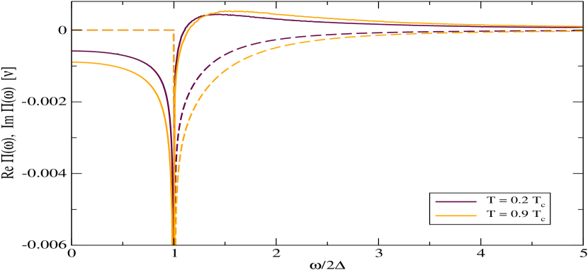
Figure 1: Dependence of the real (solid lines) and imaginary (dashed lines) parts of the pair breaking polarization tensor in units of density of states on the energy transfer in units of threshold energy $2\Delta(T)$ for fixed momentum transfer $q=0.1p_{F}$, with $p_{F}=0.1$ fm^-1, and two temperatures $T=0.2T_{c}$ (heavy lines) and $T=0.9T_{c}$ (light lines). The zero temperature gap is taken to be $\Delta(0)=1.$ MeV, $T_{c}=\Delta(0)/1.76$.

The real part of the polarization tensor follows from the dispersion (Kramers-Kronig) relation:

$${\rm Re}\Pi^{R}(\omega,\bm{q})=-\frac{1}{\pi}\int d\omega^{\prime}\frac{{\rm Im}\Pi^{R}(\omega^{\prime},\bm{q})}{\omega-\omega^{\prime}}.$$ (50)

Using these quantities one can construct an effective theory of collective excitations. Their (full, interacting) propagators are completely determined by the spectral function of the collective excitations

$$B(\omega,\bm{q})=\frac{-2{\rm Im}\Pi^{R}(\omega,\bm{q})}{\left[\omega^{2}-\bm{q}^{2}-{\rm Re}\Pi^{R}(\omega,\bm{q})\right]^{2}+{\rm Im}\Pi^{R}(\omega,\bm{q})^{2}}.$$ (51)

The dispersion relation of the collective excitations is read-off as $\omega^{2}=\bm{q}^{2}+{\rm Re}\Pi^{R}(\omega,\bm{q})$. The finite life-time effects are described by the width of the spectral function, i.e., by the function ${\rm Im}\Pi^{R}(\omega,\bm{q})$.

Figure 1 illustrates the dependence of the real and imaginary parts of the pair breaking polarization tensor on the transferred energy for fixed three-momentum transfer. The value of the Landau parameter is $f_{0}=-0.5$ Sedrakian:2006ys . The zero temperature gap at $p_{F}=0.1$ fm^-1 is $\Delta(0)=1$ MeV and $T_{c}=\Delta(0)/1.76$. The frequencies are normalized to the zero-temperature threshold frequency $2\Delta(0)$, the momentum transfer to the Fermi momentum. The real and imaginary parts of the polarization tensor scale as $q^{2}$. Their behavior at negative energies follows from their even and odd parity with respect to the energy transfer, i.e., ${\rm Re}\Pi^{R}(-\omega)={\rm Re}\Pi^{R}(\omega)$ and ${\rm Im}\Pi^{R}(-\omega)=-{\rm Im}\Pi^{R}(\omega)$. Note that the imaginary parts are identically zero below the threshold for pair breaking process $2\Delta(T)$.

Figure 2: The spectral function of density fluctuations at $T=0.2T_{c}$ (upper panel) and $T=0.9T_{c}$ (lower panel). The parameters are as in Fig. 1.

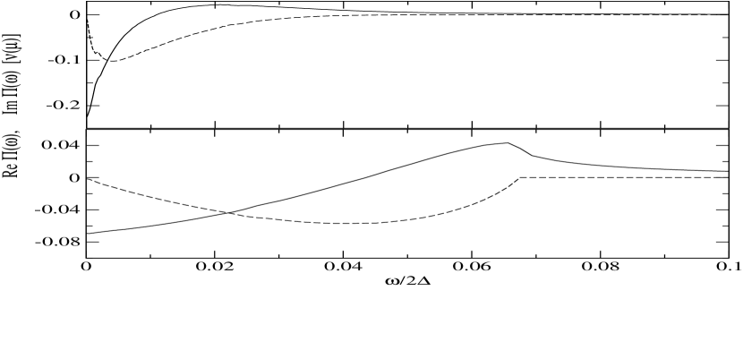
Figure 3: Dependence of the real (solid lines) and imaginary (dashed lines) parts of the scattering polarization tensor in units of density of states on the energy transfer in units of threshold energy $2\Delta(0)$ for fixed momentum transfer $q=0.1p_{F}$, with $p_{F}=0.1$ fm^-1, and two temperatures $T=0.2T_{c}$ (upper panel) and $T=0.9T_{c}$ (lower panel). The zero temperature gap is taken to be $\Delta(0)=1$ MeV, $T_{c}=\Delta(0)/1.76$.

Figure 4: The spectral function of density fluctuations at $T=0.2T_{c}$ (upper panel) and $T=0.9T_{c}$ (lower panel). The parameters are as in Fig. 1.

Figure 2 illustrates the spectral functions of pair breaking density fluctuation on the energy and momentum transfers. The parameters are the same as in Fig. 1. The form of the spectral function suggests that at low temperatures the low-momentum-transfer contribution is concentrated near the pair breaking threshold; for larger momentum transfers, modes away from the energy threshold become important. At higher temperatures ($T\leq T_{c}$) and for any given momentum transfer, the main contribution to the spectral function comes from higher energy modes and the peak values are larger in the latter regime.

III.2 Scattering response function: numerical evaluation

The scattering part of the response function is kinematically important for the space-like processes and vanishes automatically in the limit $\bm{q}\to 0$. Small momentum expansion of the previous section was found inappropriate for the scattering part of the polarization function and it was evaluated numerically by adapting the method described in Ref. Sedrakian:2004qd . On carrying out the angular integrals we are left with a one-dimensional integral over the energy. As an example, we give the expression for the elementary loop

$${\rm Im}\Pi^{\prime}_{GG}(q)\nu(p_{F})^{-1},=-\frac{\pi p_{F}T}{4q\mu_{0}}\int_{-\mu/T}^{\infty}\frac{d\xi_{p}}{T}$$

$$\Biggl{[}u_{p}^{2}u_{p+q}^{2}\frac{\epsilon_{p+q}}{\xi_{p+q}}\Bigg{|}_{x=x_{0}^{+}}\left[f(\epsilon_{p})-f(\epsilon_{p}+\omega)\right]\theta(1-|x_{0}^{+}|)$$

$$-v_{p}^{2}v_{p+q}^{2}\frac{\epsilon_{p+q}}{\xi_{p+q}}\Bigg{|}_{x=x_{0}^{-}}\left[f(\epsilon_{p})-f(\epsilon_{p}-\omega)\right]\theta(1-|x_{0}^{-}|)\Biggr{]},$$

where $\theta$ is the Heaviside step function, $x=(\bm{p}\cdot\bm{q})/|\bm{p}||\bm{q}|$, and $x_{0}^{\pm}$ is the $x$ value satisfying the equation $\pm\omega+\epsilon_{p}-\epsilon_{p+q}=0$ and the prime refers to the scattering part. The expressions for the scattering parts of the polarization tensors $\Pi^{\prime}_{XX^{\prime}}(q)$ are similar to Eq. (III.2), but involve different combinations of coherence factors. The real parts are obtained from the dispersion relation (50).

Figure 3 shows the real and imaginary parts of the scattering polarization tensor at two temperatures and for fixed momentum transfer. Figure 4 shows the spectral function derived from the scattering polarization tensor. It is seen that the modes with energies within the breaking threshold $\omega\leq 2\Delta(0)$ are relevant for scattering processes, as opposed to the pair breaking case where only the modes with $\omega\geq 2\Delta(0)$ emerge. This justifies the separation of the modes into two classes. The peak values are larger at higher temperatures $T\leq T_{c}$, as is the case for the pair breaking response.

III.3 Unpaired and uncorrelated limits

Here we wish to obtain the unpaired ($T>T_{c}$) limit of the polarization function (24). This amounts to setting the coherence factors in Eq. (25)–(28) to their values in the normal state

$$u_{p}=1,\quad v_{p}=0.$$ (53)

It follows then from Eq. (26) that $\Pi_{FG}=0=\Pi_{GF}$ and, therefore, ${\cal B}=0$. Setting ${\cal B}=0$ in Eq. (24) and noting that ${\cal C}\neq 0$, since $\Pi_{G^{\dagger}G}\neq 0$, we obtain

$$\Pi_{RPA}(q)=\frac{{\cal A}(q)}{1-v_{ph}{\cal A}(q)},$$ (54)

where the function ${\cal A}(q)$ in the unpaired state reduces to

$${\cal A}(q)=\Pi_{GG}(q,\Delta=0)=g\int\frac{d^{3}p}{(2\pi)^{3}}\frac{f(\epsilon_{p})-f(\epsilon_{k})}{\omega+\epsilon_{p}-\epsilon_{k}+i\delta}.$$

Equations (54) and (III.3) are the standard expressions for the polarization tensor of a Fermi liquid in the random phase approximation (RPA). The free Fermi gas result follows on setting $v_{ph}=0$ in Eq. (54):

$$\Pi_{free}(q)=g\int\frac{d^{3}p}{(2\pi)^{3}}\frac{f(\epsilon_{p})-f(\epsilon_{k})}{\omega+\epsilon_{p}-\epsilon_{k}+i\delta}.$$ (56)

Clearly, the pair-braking contribution vanishes as $T\to T_{c}^{(-)}$. The scattering contribution at $T\geq T_{c}$ reproduces the unpaired and uncorrelated limits, as it should.

IV Conclusions

In this article we have carried out several steps in the program aimed at understanding the polarization tensor of pair-correlated neutron and nuclear matter by (i) constructing a low-transfered-momentum approximation to the pair breaking polarization tensor and (ii) by numerically evaluating the scattering part of the polarization tensor.

Our main result is that the low-momentum expansion of the pair breaking polarization tensor starts at quadratic order in the ratio of the momentum-transfer to the Fermi momentum. The expansion coefficient is universal, i.e., depends only the two relevant scales: the Fermi energy and the pairing gap. We also clarified the structure of the integral equations for the vertex functions when the particle-particle and particle-hole interactions do not coincide and verified explicitly that the unpaired and uncorrelated limits are recovered.

Further steps will require a verification of the convergence of the series by a comparison of our analytical results with an exact numerical evaluation of the response functions. The rate of series convergence can be checked by computing the next-to-leading-order contribution. Further refinements could include finite range interactions, tensor forces, and so on. The new numerical and analytical methods, discussed in this article, could be useful in the studies of the response functions of pair-correlated fermionic systems in general.

The main implication of our study concerns the neutrino emissivity via the vector current pair breaking bremsstrahlung, which are phenomenologically important in the physics of neutron star cooling and superbursts in accreting neutron stars Brown:2009kw ; Page:2009fu ; Gupta:2006fd . Our results suggest that the vector current contribution to the process

$$\{nn\}\to\{nn\}+\nu+\bar{\nu},$$ (57)

where $\{nn\}$ refers to the pair correlated state, $\nu$ and $\bar{\nu}$ to the neutrino and antineutrino, is suppressed to a lesser degree, than suggested in the recent literature Leinson:2006gf ; Kolomeitsev:2008mc . However, further studies indicated above are needed to draw a final conclusion on the relative importance of this vector current neutrino emission process (57).

Appendix A Expanding the functions ${\cal A}(q)$, ${\cal B}(q)$, and ${\cal C}(q)$

We write each of these functions as a product of an appropriate coherence factor and corresponding statistical factor

$${\cal A}(q) = \int\frac{d^{3}p}{(2\pi)^{3}}a(\bm{p},\bm{q},\omega)L(\bm{p},\bm{q},\omega),$$ (58)

$${\cal B}(q) = \Delta\omega\int\frac{d^{3}p}{(2\pi)^{3}}\frac{1}{\epsilon_{p}}L(\bm{p},\bm{q},\omega),$$ (59)

$${\cal C}(q) = -\int\frac{d^{3}p}{(2\pi)^{3}}c(\bm{p},\bm{q},\omega)L(\bm{p},\bm{q},\omega)$$ (60)

$$- \int\frac{d^{3}p}{(2\pi)^{3}}\frac{1}{2\epsilon_{p}}\left[1-2f(\epsilon_{p})\right],$$

where

$$a(\bm{p},\bm{q},\omega) = \frac{\epsilon_{p}+\epsilon_{p+q}}{2}\left(1-\frac{\xi_{p}\xi_{p+q}}{\epsilon_{p}\epsilon_{p+q}}+\frac{\Delta^{2}}{\epsilon_{p}\epsilon_{p+q}}\right),$$

$$c(\bm{p},\bm{q},\omega) = \frac{\epsilon_{p}+\epsilon_{p+q}}{2}\left(1+\frac{\xi_{p}\xi_{p+q}}{\epsilon_{p}\epsilon_{p+q}}+\frac{\Delta^{2}}{\epsilon_{p}\epsilon_{p+q}}\right),$$

$$L(\bm{p},\bm{q},\omega) = \frac{1-f(\epsilon_{p})-f(\epsilon_{p+q})}{(\omega+i\delta)^{2}-(\epsilon_{p}+\epsilon_{p+q})^{2}}.$$ (63)

Next we expand these functions in powers of small parameter $y$ to order $O(y^{2})$

$$a(\bm{p},\bm{q},\omega) = \frac{2\Delta^{2}}{\epsilon_{p}}-\frac{2\Delta^{2}\,\mu\,\xi_{p}}{\epsilon_{p}^{3}}~{}x~{}y$$ (64)

$$+ \frac{\Delta^{2}\,\mu\,\xi_{p}}{\epsilon_{p}^{5}}(6\mu\xi_{p}x^{2}-\epsilon_{p}^{2})~{}y^{2},$$

$$c(\bm{p},\bm{q},\omega) = 2\epsilon_{p}+\frac{2\mu\xi_{p}}{\epsilon_{p}}~{}x~{}y+\frac{\mu\,\xi_{p}}{\epsilon_{p}}~{}y^{2},$$ (65)

$$L(\bm{p},\bm{q},\omega) = L_{0}+L_{1}xy+L_{2}y^{2},$$ (66)

where the coefficients of the expansion (66) can be written using the shorthand expressions $D\equiv\omega^{2}-4\epsilon_{p}^{2}$ and $\zeta\equiv\epsilon_{p}/2T$ as

$$L_{0} = \frac{\,\tanh\,\zeta}{D+i\delta},$$ (67)

$$L_{1} = 8\,\mu\,{\xi_{p}}\,\frac{\tanh\,\zeta}{{\left(D+i\delta\right)}^{2}}+\frac{\mu\,{\xi_{p}}}{2{\epsilon_{p}}\,T}\frac{{\rm sech}^{2}\,\zeta}{(D+i\delta)},$$ (68)

$$L_{2} = \frac{4\,{\mu}^{2}\,x^{2}\,{{\xi_{p}}}^{2}\,{\rm sech}^{2}\,\zeta}{{\epsilon_{p}}\,T\,{\left(D+i\delta\right)}^{2}}+\frac{{\mu}^{2}\,x^{2}\,{\rm sech}^{2}\,\zeta}{2\,{\epsilon_{p}}\,T\,\left(D+i\delta\right)}$$ (69)

$$+ \frac{\mu\,{\xi_{p}}{\rm sech}^{2}\,\zeta}{4\,{\epsilon_{p}}\,T\,\left(D+i\delta\right)}-\frac{{\mu}^{2}\,x^{2}\,{{\xi_{p}}}^{2}\,{\rm sech}^{2}\,\zeta}{2\,{{\epsilon_{p}}}^{3}\,T\,\left(D+i\delta\right)}$$

$$+ \frac{64\,{\mu}^{2}\,x^{2}\,{{\xi_{p}}}^{2}\,\tanh\,\zeta}{{\left(D+i\delta\right)}^{3}}+\frac{8\,{\mu}^{2}\,x^{2}\,\tanh\,\zeta}{{\left(D+i\delta\right)}^{2}}$$

$$+ \frac{4\,\mu\,{\xi_{p}}\,\tanh\zeta}{{\left(D+i\delta\right)}^{2}}-\frac{4\,{\mu}^{2}\,x^{2}\,{{\xi_{p}}}^{2}\,\tanh\zeta}{{{\epsilon_{p}}}^{2}\,{\left(D+i\delta\right)}^{2}}$$

$$- \frac{{\mu}^{2}\,x^{2}\,{{\xi_{p}}}^{2}\,\tanh\zeta\,{\rm sech}^{2}\zeta}{2\,{{\epsilon_{p}}}^{2}\,T^{2}\,\left(D+i\delta\right)},$$

where ${\rm sech}^{2}\left(x\right)\equiv 1-\tanh\left(x\right)^{2}$. On substituting Eqs. (64) and (66) in Eq. (58) we obtain

$${\cal A}(q) = \int\frac{d^{3}p}{(2\pi)^{3}}\Biggl{[}\frac{2\Delta^{2}}{\epsilon_{p}}L_{0}+\frac{2\Delta^{2}}{\epsilon_{p}}L_{2}y^{2}$$ (70)

$$- \frac{2\Delta^{2}\,\mu\,\xi_{p}}{\epsilon_{p}^{3}}~{}L_{1}~{}x^{2}~{}y^{2}+\frac{\Delta^{2}\,\mu\,\xi_{p}}{\epsilon_{p}^{5}}(6\mu\xi_{p}x^{2}-\epsilon_{p}^{2})L_{0}~{}y^{2}\Biggr{]}$$

$$= {\cal A}_{0}(q)+{\cal A}_{2}(q)y^{2}+O(y^{4}).$$

The terms that are odd in $x$ drop out on integration in symmetrical limits. Similarly,

$${\cal C}(q) = -\int\frac{d^{3}p}{(2\pi)^{3}}\Biggl{[}2\epsilon_{p}L_{0}+\frac{2\mu\xi_{p}}{\epsilon_{p}}L_{1}~{}x^{2}~{}y^{2}+\frac{\mu\,\xi_{p}}{\epsilon_{p}}~{}L_{0}~{}y^{2}$$ (71)

$$+ 2\epsilon_{p}L_{2}y^{2}\Biggr{]}-\int\frac{d^{3}p}{(2\pi)^{3}}\frac{1}{2\epsilon_{p}}\left[1-2f(\epsilon_{p})\right].$$

We further use the relation

$$-\int\frac{d^{3}p}{(2\pi)^{3}}2\epsilon_{p}L_{0}-\int\frac{d^{3}p}{(2\pi)^{3}}\frac{1}{2\epsilon_{p}}\left[1-2f(\epsilon_{p})\right]$$

$$\hskip 85.35826pt=-\frac{\omega^{2}}{2}\int\frac{d^{3}p}{(2\pi)^{3}}\frac{1}{\epsilon_{p}}L_{0}\,$$ (72)

to write

$${\cal C}(q) = -\frac{\omega^{2}}{2}\int\frac{d^{3}p}{(2\pi)^{3}}\frac{1}{\epsilon_{p}}L_{0}-\int\frac{d^{3}p}{(2\pi)^{3}}\Biggl{[}\frac{2\mu\xi_{p}}{\epsilon_{p}}L_{1}~{}x^{2}~{}y^{2}$$

$$+ \frac{\mu\,\xi_{p}}{\epsilon_{p}}~{}L_{0}~{}y^{2}+2\epsilon_{p}L_{2}y^{2}\Biggr{]}={\cal C}_{0}(q)+{\cal C}_{2}(q)y^{2}.$$

Finally,

$${\cal B}(q) = \Delta\omega\int\frac{d^{3}p}{(2\pi)^{3}}\frac{1}{\epsilon_{p}}(L_{0}+L_{2}~{}y^{2})={\cal B}_{0}(q)+{\cal B}_{2}(q)y^{2},$$

and ${{\cal A}_{0}}/{{\cal C}_{0}}=-{4\Delta^{2}}/{\omega^{2}},$ and ${{\cal B}_{0}}/{{\cal C}_{0}}=-{2\Delta}/{\omega}$.

Appendix B Evaluating phase-space integrals

Here we evaluate the integrals (45)–(47), which are given as

$$I_{0} = \nu(p_{F})^{-1}\mu\,\int\frac{d^{3}p}{(2\pi)^{3}}\frac{\xi_{p}}{\epsilon_{p}^{3}}\left[\frac{4\epsilon_{p}^{2}}{\omega^{2}}-1+\frac{6\mu\xi_{p}}{\epsilon_{p}^{2}}x^{2}\right]L_{0},$$

$$I_{1} = 2\nu(p_{F})^{-1}\mu\int\frac{d^{3}p}{(2\pi)^{3}}\frac{\xi_{p}}{\epsilon_{p}^{3}}\left[\frac{4\epsilon_{p}^{2}}{\omega^{2}}-1\right]~{}L_{1}x^{2},$$ (76)

$$I_{2} = 2\nu(p_{F})^{-1}\int\frac{d^{3}p}{(2\pi)^{3}}\frac{1}{\epsilon_{p}}\left[\frac{4\epsilon_{p}^{2}}{\omega^{2}}-1\right]L_{2}(x).$$ (77)

After carrying out the angular integrals we obtain

$$I_{0} = \nu(p_{F})^{-1}\mu\,\int\frac{dpp^{2}}{2\pi^{2}}\frac{\xi_{p}}{\epsilon_{p}^{3}}\left[\frac{4\epsilon_{p}^{2}}{\omega^{2}}-1+\frac{2\mu\xi_{p}}{\epsilon_{p}^{2}}\right]L_{0},$$

$$I_{1} = \frac{2}{3}\nu(p_{F})^{-1}\mu\int\frac{dpp^{2}}{2\pi^{2}}\frac{\xi_{p}}{\epsilon_{p}^{3}}\left[\frac{4\epsilon_{p}^{2}}{\omega^{2}}-1\right]~{}L_{1},$$ (79)

$$I_{2} = 2\nu(p_{F})^{-1}\int\frac{dpp^{2}}{2\pi^{2}}\frac{1}{\epsilon_{p}}\left[\frac{4\epsilon_{p}^{2}}{\omega^{2}}-1\right]\langle L_{2}(x)\rangle,$$ (80)

where $\langle L_{2}\rangle$ is the angle integrated loop $L_{2}$, which is obtain from (69) via the substitution $x^{2}=1/3$. Using the transformation $dpp^{2}=m^{*}p_{F}d(p^{2}/2m^{*})=m^{*}p_{F}d\xi_{p},$ and the relation $\epsilon_{p}d\epsilon_{p}=\xi_{p}d\xi_{p}$ we obtain

$$I_{0} = \mu\,\int_{\Delta}^{\infty}{d\epsilon_{p}}\frac{1}{\epsilon_{p}^{2}}\left[\frac{4\epsilon_{p}^{2}}{\omega^{2}}-1+\frac{2\mu\xi_{p}}{\epsilon_{p}^{2}}\right]L_{0},$$ (81)

$$I_{1} = \frac{2\mu}{3}\int_{\Delta}^{\infty}{d\epsilon_{p}}\frac{1}{\epsilon_{p}^{2}}\left[\frac{4\epsilon_{p}^{2}}{\omega^{2}}-1\right]~{}L_{1},$$ (82)

$$I_{2} = 2\int_{\Delta}^{\infty}{d\epsilon_{p}}\frac{1}{\xi_{p}}\left[\frac{4\epsilon_{p}^{2}}{\omega^{2}}-1\right]\langle L_{2}(x)\rangle.$$ (83)

To make further progress we need to separate the real and imaginary parts of the integrals. We shall first compute the imaginary parts. They are extracted with the help of the identity

$$\frac{1}{(D+i\delta)^{n+1}}=\frac{P}{D^{n+1}}-i\pi\frac{(-1)^{n}}{n!}\delta^{(n)}(D),$$ (84)

where $P$ denotes the principal value and $\delta^{(n)}(D)$ is the $n$-th derivative of the delta function.

For positive $\omega$ the integral (B) gives 

$${\rm Im}I_{0} = -\pi\mu\,\int_{\Delta}^{\infty}{d\epsilon_{p}}\frac{1}{\epsilon_{p}^{2}}\Biggl{[}\frac{4\epsilon_{p}^{2}}{\omega^{2}}-1$$

$$+ \frac{2\mu\xi_{p}}{\epsilon_{p}^{2}}\Biggr{]}\tanh\left(\frac{\epsilon_{p}}{2\,T}\right)\delta(\omega^{2}-4\epsilon_{p}^{2})$$

$$= -8\pi\mu^{2}\,\frac{\sqrt{\omega^{2}-4\Delta^{2}}~{}{\rm sgn}(\omega)}{\omega^{5}}\tanh\left(\frac{\omega}{4\,T}\right)\,\theta(\omega-2\Delta).$$

Consider the integral (76). First, note that the term $\propto D^{-1}$ vanishes, since the delta function enforces $\omega^{2}=4\epsilon_{p}^{2}$. After dropping this term we are left with the integral

$${\rm Im}I_{1} = \frac{16\pi\mu^{2}}{3}\int_{\Delta}^{\infty}d\epsilon_{p}\frac{1}{\epsilon_{p}^{2}}\left(\frac{4\epsilon_{p}^{2}}{\omega^{2}}-1\right)\sqrt{\epsilon_{p}^{2}-\Delta^{2}}$$ (86)

$$\tanh\left(\frac{\epsilon_{p}}{2T}\right)\delta^{(1)}(\omega^{2}-4\epsilon_{p}^{2}).$$

This and similar integrals, which contain derivatives of the delta function, are computed via the formula

$$\int f(x)\delta^{n}(x-a)dx=(-)^{n}f^{(n)}(a).$$ (87)

The result of integration is

$${\rm Im}I_{1}=-\frac{8\pi\mu^{2}}{3}\frac{\sqrt{\omega^{2}-4\Delta^{2}}~{}{\rm sgn}(\omega)}{\omega^{5}}\tanh\left(\frac{\omega}{4T}\right)\,\theta(\omega-2\Delta)\,.$$ (88)

In the integral (77) we again omit terms $\propto D^{-1}$, since their prefactors are zero after integration. After inserting $x^{2}=1/3$ in the remainder we obtain

$${\rm Im}I_{2} = \frac{8\pi}{3}\int_{\Delta}^{\infty}d\epsilon_{p}\,\left[\frac{4\epsilon_{p}^{2}}{\omega^{2}}-1\right]\Bigg{\{}\frac{\mu^{2}\sqrt{\epsilon_{p}^{2}-\Delta^{2}}}{\epsilon_{p}\,T}{\rm sech}^{2}\left(\frac{\epsilon_{p}}{2T}\right)+\frac{2}{\sqrt{\epsilon_{p}^{2}-\Delta^{2}}}\mu^{2}\tanh\left(\frac{\epsilon_{p}}{2T}\right)$$ (89)

$$\hskip 56.9055pt+3\mu\tanh\left(\frac{\epsilon_{p}}{2T}\right)-\frac{\mu^{2}\sqrt{\epsilon_{p}^{2}-\Delta^{2}}}{\epsilon_{p}^{2}}\tanh\left(\frac{\epsilon_{p}}{2T}\right)\Bigg{\}}\,\delta^{(1)}(\omega^{2}-4\epsilon_{p}^{2})$$

$$-\,\frac{64\pi\mu^{2}}{3}\int_{\Delta}^{\infty}d\epsilon_{p}\,\left[\frac{4\epsilon_{p}^{2}}{\omega^{2}}-1\right]\sqrt{\epsilon_{p}^{2}-\Delta^{2}}\tanh\left(\frac{\epsilon_{p}}{2T}\right)\delta^{(2)}(\omega^{2}-4\epsilon_{p}^{2})\,.$$

Applying Eq. (87) we obtain

$${\rm Im}I_{2} = -\frac{\pi\mu~{}{\rm sgn}(\omega)}{3T\omega^{5}\sqrt{\omega^{2}-4\Delta^{2}}}\,{\rm sech}^{2}\left(\frac{\omega}{4T}\right)\Bigg{\{}T\,[24\Delta^{2}\mu+\omega^{2}\,(2\mu+3\sqrt{\omega^{2}-4\Delta^{2}})]\sinh\left(\frac{\omega}{2T}\right)+4\mu\omega\,(\omega^{2}-4\Delta^{2})\Bigg{\}}\,\theta(\omega-2\Delta)\,.$$

Finally, adding the three integrals (B), (88), and (B) we obtain Eq. (III.1) of the main text.

References

• (1) A. B. Migdal, Theory of Finite Fermi Systems and Applications to Atomic Nuclei (Interscience, London, 1967).
• (2) A. Sedrakian, H. Müther and P. Schuck, “Vertex renormalization in weak decays of Cooper pairs and cooling compact stars,” Phys. Rev.  C 76, 055805 (2007) [arXiv:astro-ph/0611676].
• (3) E. E. Kolomeitsev and D. N. Voskresensky, “Neutrino emission due to Cooper-pair recombination in neutron stars revisited,” Phys. Rev.  C 77, 065808 (2008) [arXiv:0802.1404 [nucl-th]].
• (4) A. W. Steiner and S. Reddy, “Superfluid Response and the Neutrino Emissivity of Neutron Matter,” Phys. Rev.  C 79, 015802 (2009) [arXiv:0804.0593 [nucl-th]].
• (5) L. B. Leinson, “Superfluid response and the neutrino emissivity of baryon matter. Fermi-liquid effects,” Phys. Rev.  C 79, 045502 (2009) [arXiv:0904.0320 [astro-ph.HE]].
• (6) J. Kundu and S. Reddy, “Neutrino scattering off pair-breaking and collective excitations in superfluid neutron matter and in color-flavor locked quark matter,” Phys. Rev.  C 70, 055803 (2004) [arXiv:nucl-th/0405055].
• (7) E. Olsson, P. Haensel and C. J. Pethick, “Static response of Fermi liquids with tensor interactions,” Phys. Rev.  C 70, 025804 (2004) [arXiv:nucl-th/0403066].
• (8) G. I. Lykasov, E. Olsson and C. J. Pethick, “Long-wavelength spin- and spin-isospin correlations in nucleon matter,” Phys. Rev.  C 72, 025805 (2005) [arXiv:nucl-th/0502026].
• (9) J. Margueron, N. Van Giai and J. Navarro, “Nuclear response functions in homogeneous matter with finite range effective interactions,” Phys. Rev.  C 72, 034311 (2005) [arXiv:nucl-th/0507053].
• (10) M. Baldo and C. Ducoin, “Elementary excitations in homogeneous neutron star matter,” Phys. Rev.  C 79, 035801 (2009) [arXiv:0811.0604 [nucl-th]].
• (11) A. Burrows and R. F. Sawyer, “Many-body corrections to charged-current neutrino absorption rates in nuclear matter,” Phys. Rev.  C 59, 510 (1999) [arXiv:astro-ph/9804264].
• (12) A. Sedrakian and A. E. L. Dieperink, “Coherence effects and neutrino pair bremsstrahlung in neutron stars,” Phys. Lett.  B 463, 145 (1999) [arXiv:nucl-th/9905039].
• (13) A. Sedrakian and A. E. L. Dieperink, “Coherent neutrino radiation in supernovae at two loops,” Phys. Rev.  D 62, 083002 (2000) [arXiv:astro-ph/0002228].
• (14) A. Sedrakian, “The physics of dense hadronic matter and compact stars,” Prog. Part. Nucl. Phys.  58, 168 (2007) [arXiv:nucl-th/0601086].
• (15) E. F. Brown and A. Cumming, “Mapping crustal heating with the cooling lightcurves of quasi-persistent transients,” Astrophys. J.  698, 1020 (2009) [arXiv:0901.3115 [astro-ph.SR]].
• (16) D. Page, J. M. Lattimer, M. Prakash and A. W. Steiner, “Neutrino Emission from Cooper Pairs and Minimal Cooling of Neutron Stars,” Astrophys. J.  707, 1131 (2009) arXiv:0906.1621 [astro-ph.SR].
• (17) S. Gupta, E. F. Brown, H. Schatz, P. Moeller and K. L. Kratz, “Heating in the Accreted Neutron Star Ocean: Implications for Superburst Ignition,” Astrophys. J.  662, 1188 (2007) [arXiv:astro-ph/0609828].
• (18) L. B. Leinson and A. Perez, “Vector current conservation and neutrino emission from singlet-paired baryons in neutron stars,” Phys. Lett.  B 638, 114 (2006) [arXiv:astro-ph/0606651].
• (19) A. Sedrakian, T. T. S. Kuo, H. Müther and P. Schuck, “Pairing in nuclear systems with effective Gogny and $V_{low-k}$ interactions,” Phys. Lett.  B 576, 68 (2003) [arXiv:nucl-th/0308068].
• (20) A. Sedrakian, “Direct Urca neutrino radiation from superfluid baryonic matter,” Phys. Lett.  B 607, 27 (2005) [arXiv:nucl-th/0411061].