Almost Prime Pythagorean Triples in Thin Orbits

Abstract.

For the ternary quadratic form $Q({\bf x})=x^{2}+y^{2}-z^{2}$ and a non-zero Pythagorean triple ${{\bf x}}_{0}\in\mathbb{Z}^{3}$ lying on the cone $Q({{\bf x}})=0$, we consider an orbit ${\mathcal{O}}={{\bf x}}_{0}\Gamma$ of a finitely generated subgroup $\Gamma<\operatorname{SO}_{Q}(\mathbb{Z})$ with critical exponent exceeding $1/2$.

We find infinitely many Pythagorean triples in ${\mathcal{O}}$ whose hypotenuse, area, and product of side lengths have few prime factors, where “few” is explicitly quantified. We also compute the asymptotic of the number of such Pythagorean triples of norm at most $T$, up to bounded constants.

1. Introduction

1.1. The Affine Linear Sieve

In [BGS06], Bourgain, Gamburd, and Sarnak introduced the Affine Linear Sieve, which extends some classical sieve methods to thin orbits of non-abelian group actions. Its input is a pair $({\mathcal{O}},F)$, where

1. ${\mathcal{O}}$ is a discrete orbit, ${\mathcal{O}}={\bf x}_{0}\cdot\Gamma$, generated by a discrete subgroup $\Gamma$ of a linear group $G$. It is called “thin” if the volume of $\Gamma\backslash G$ is infinite; and

2. $F$ is a polynomial, taking integer values on ${\mathcal{O}}$.

Given the pair $({\mathcal{O}},F)$, the Affine Linear Sieve attempts to output a number $R=R({\mathcal{O}},F)$ as small as possible so that there are infinitely many integers $n\in F({\mathcal{O}})$, with $n$ having at most $R$ prime factors.

A special case of their main result is the following.

Theorem 1.1 ([BGS06, BGS08]).

Let $G<\operatorname{GL}_{n}(\mathbb{R})$ be a $\mathbb{Q}$-form of $\operatorname{SL}_{2}$, and let $\Gamma$ be a non-elementary subgroup of $G\cap\operatorname{GL}_{n}(\mathbb{Z})$. Let ${\mathcal{O}}$ be an orbit ${{\bf x}}_{0}\Gamma$ for some ${{\bf x}}_{0}\in\mathbb{Z}^{n}\setminus\{0\}$ and $F$ any polynomial which is integral on ${\mathcal{O}}$. Then there exists a number

$$R=R({\mathcal{O}},F)<\infty$$

such that there are infinitely many ${\bf x}\in{\mathcal{O}}$ with $F({\bf x})$ having at most $R$ prime factors. Moreover the set of such ${\bf x}$ is Zariski dense in the Zariski closure of ${\mathcal{O}}$.

Remark 1.2.

As described in [BGS08, §2], Lagarias gave evidence that the result above may be false if one drops the condition that $\Gamma$ is non-elementary.

For various special cases of $({\mathcal{O}},F)$, one can say more than just $R<\infty$; one can give explicit, “reasonable” values of $R({\mathcal{O}},F)$. This was achieved with some restrictions in [Kon07, Kon09], and it is our present goal to improve the results there in a more general setting.

In order to remove local obstructions which would increase $R$ for trivial reasons, we will impose the strong primitivity condition on $({\mathcal{O}},F)$.

Definition 1.3.

For a subset ${\mathcal{O}}\subset\mathbb{Z}^{n}$ and a polynomial $F(x_{1},\cdots,x_{n})$ taking integral values on ${\mathcal{O}}$, the pair $({\mathcal{O}},F)$ is called strongly primitive if for every integer $q\geq 2$ there is an ${{\bf x}}\in{\mathcal{O}}$ such that

$$F({{\bf x}})\neq 0\quad(\operatorname{mod}q).$$

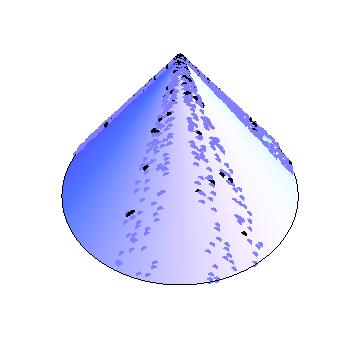
Hypotenuse is prime

Hypotenuse is composite

Figure 1. A thin orbit ${\mathcal{O}}$ of Pythagorean triples, sifted by hypotenuse, $F(x,y,z)=z$. The darker points denote those triples whose hypotenuse is prime.

Remark 1.4.

The weaker condition of primitivity requires the above for $q$ prime. See [BGS08, §2] for an example of $({\mathcal{O}},F)$ which is primitive but not strongly primitive.

To present a concrete number $R({\mathcal{O}},F)$, we will consider the quadratic form

$$Q({{\bf x}})=x^{2}+y^{2}-z^{2}.$$

Hence a non-zero vector ${{\bf x}}\in\mathbb{Z}^{3}$ is a Pythagorean triple if $Q({\bf x})=0$. Let $G=\operatorname{SO}_{Q}(\mathbb{R})$ be the special orthogonal group preserving $Q$ with real entries. For a discrete subgroup $\Gamma$ of $G$, the critical exponent $0\leq\delta_{\Gamma}\leq 1$ of $\Gamma$ is defined to be the abscissa of convergence of the Poincare series:

$$L_{\Gamma}(s):=\sum_{\gamma\in\Gamma}\|\gamma\|^{-s}$$

for any norm $\|\cdot\|$ on the vector space $\operatorname{M}_{3}(\mathbb{R})$ of $3\times 3$ matrices. We remark that $\Gamma$ is non-elementary if and only if $\delta_{\Gamma}>0$. Moreover if $\Gamma$ is finitely-generated, then $\Gamma$ is of finite co-volume in $G$ if and only if $\delta_{\Gamma}=1$ [Pat76].

The detailed statement of our main result is given in Theorem 2.23. The following is a special case:

Theorem 1.5.

Let $\Gamma<\operatorname{SO}_{Q}(\mathbb{Z})$ be a finitely generated subgroup and set

$${\mathcal{O}}:=(3,4,5)\Gamma.$$

Let the polynomial $F$ be one of

$$\begin{cases}\text{the hypotenuse: }&F_{\mathcal{H}}({{\bf x}}):=z;\\ \text{the ``area'': }&F_{\mathcal{A}}({{\bf x}}):=\frac{1}{12}xy;\\ \text{the product of coordinates : }&F_{\mathcal{C}}({{\bf x}}):=\frac{1}{60}xyz.\end{cases}$$

We assume that the pair $({\mathcal{O}},F)$ is strongly primitive and that

$$\delta>\begin{cases}0.9992&\text{ if $F=F_{\mathcal{H}}$;}\\ 0.99995&\text{ if $F=F_{\mathcal{A}}$;}\\ 0.99677&\text{ if $F=F_{\mathcal{C}}$. }\end{cases}$$

Then the following hold:

1. For infinitely many ${{\bf x}}\in{\mathcal{O}}$, the integer $F({{\bf x}})$ has at most $R=R({\mathcal{O}},F)$ prime factors, where

   $$R=\begin{cases}14&\text{if $F=F_{\mathcal{H}}$};\\ 25&\text{ if $F=F_{\mathcal{A}}$;}\\ 29&\text{ if $F=F_{\mathcal{C}}$.}\end{cases}$$

2. We have

   $$\#\{{{\bf x}}\in{\mathcal{O}}:\|x\|<T,\text{ $F({{\bf x}})$ has at most $R({\mathcal{O}},F)$ prime factors}\}\asymp{T^{\delta_{\Gamma}}\over(\log T)^{\kappa}},$$

   where $\|\cdot\|$ is any norm on $\mathbb{R}^{3}$ and the sieve dimension $\kappa$ is

   $$\kappa=\begin{cases}1&\text{ if $F=F_{\mathcal{H}}$;}\\ 4&\text{ if $F=F_{\mathcal{A}}$;}\\ 5&\text{ if $F=F_{\mathcal{C}}$.}\end{cases}$$

   In particular, the set of ${{\bf x}}\in{\mathcal{O}}$ such that $F({{\bf x}})$ has at most $R({\mathcal{O}},F)$ prime factors is Zariski dense in the cone $Q=0$.

Remark 1.6.

The functions $F_{\mathcal{A}}$ and $F_{\mathcal{C}}$ satisfy $F(3,4,5)=1$; hence the pair $({\mathcal{O}},F)$ is strongly primitive regardless of the choice of the group $\Gamma$. For the hypotenuse, $F_{\mathcal{H}}$, one must check, given $\Gamma$, that the pair $({\mathcal{O}},F)$ is strongly primitive.

Remark 1.7.

The above theorem was proved in [Kon09] assuming that $\Gamma$ contains a non-trivial (parabolic) stabilizer of $(3,4,5)$. In this case, the orbit ${\mathcal{O}}$ contains an injection of affine space, and hence standard sieve methods [Iwa78] also produce integral points with few prime factors. Some of the most interesting cases which cannot be dealt with using standard methods and are now covered by our results are the so-called Schottky groups; these are groups generated by finitely many hyperbolic elements.

1.2. A Counting theorem

In order to sieve almost primes in a given orbit, one must know how to count points on such orbits, which we obtain without assuming the arithmetic condition on $\Gamma$.

Theorem 1.8.

Let $Q$ be any ternary indefinite quadratic form, $G=\operatorname{SO}_{Q}(\mathbb{R})$, and $\Gamma<G$ a finitely generated discrete subgroup with $\delta_{\Gamma}>1/2$. Let ${{\bf x}}_{0}\in\mathbb{R}^{3}$ be a non-zero vector lying on the cone $Q=0$ such that the orbit ${\mathcal{O}}={{\bf x}}_{0}\cdot\Gamma$ is discrete.

Then there exist a constant $c_{0}>0$ and some $\zeta>0$ such that as $T\to\infty$,

$$\#\{{{\bf x}}\in{\mathcal{O}}:\|{{\bf x}}\|<T\}=c_{0}\cdot T^{\delta}+O(T^{\delta-\zeta}).$$

The norm $\|\cdot\|$ above is Euclidean.

Remark 1.9.

Let $N_{0}$ denote the (unipotent) stabilizer of ${{\bf x}}_{0}$ in $G$. The Theorem 1.8 was proved in [Kon09] under the further assumption that $\Gamma\cap N_{0}$ is a lattice in $N_{0}$.

1.3. Expanding Closed Horocycles

The main difference between this paper and [Kon09] is the method used to establish counting theorems such as Theorem 1.8. While [Kon09] uses abstract operator theory, in the present work we prove the effective equidistribution of expanding closed horocycles on a hyperbolic surface $X$, allowing not only $X$ to have infinite volume, but also allowing the closed horocycle to be infinite in length.

Let $G=\operatorname{SL}_{2}(\mathbb{R})$ and write the Iwasawa decomposition $G=NAK$ with

$$N=\left\{n_{x}=\begin{pmatrix}1&x\\ 0&1\end{pmatrix}:x\in\mathbb{R}\right\},\quad A=\left\{a_{y}=\begin{pmatrix}\sqrt{y}&0\\ 0&1/\sqrt{y}\end{pmatrix}:y>0\right\},$$ (1.10)

and $K=\operatorname{SO}_{2}(\mathbb{R})$.

We use the upper half plane $\mathbb{H}=\{z=x+iy:y>0\}$ as a model for the hyperbolic plane with the metric $\frac{\sqrt{dx^{2}+dy^{2}}}{y}$. The group $G$ acts on $\mathbb{H}$ by fractional linear transformations which give arise all orientation preserving isometries of $\mathbb{H}$:

$$\begin{pmatrix}a&b\\ c&d\end{pmatrix}z=\frac{az+b}{cz+d}$$

for $\operatorname{Im}(z)>0$. We compute:

$$n_{x}a_{y}(i)=x+iy.$$

Let $\Gamma<G$ be a finitely generated discrete subgroup with $\delta_{\Gamma}>1/2$. Assume that the horocycle $(\Gamma\cap N)\backslash N$ is closed in $X:=\Gamma\backslash G$, or equivalently the image of $N(i)=\{x+i:x\in\mathbb{R}\}$ is closed in $\Gamma\backslash\mathbb{H}$ under the canonical projection $\mathbb{H}\to\Gamma\backslash\mathbb{H}$. Geometrically, this is isomorphic to either a line $\mathbb{R}$ or to a circle $\mathbb{R}/\mathbb{Z}$, depending on whether or not $\Gamma\cap N$ is trivial. We push the closed horocycle $(N\cap\Gamma)\backslash N(i)$ in the orthogonal direction $a_{y}$, and are concerned with its asymptotic distribution near the boundary, corresponding to $y\to 0$.

Let $X=\Gamma\backslash\mathbb{H}$ and consider the Laplace operator $\Delta=-y^{2}(\partial_{xx}+\partial_{yy})$. By Patterson [Pat76] and Lax-Phillips [LP82], the spectral resolution of $\Delta$ acting on $L^{2}(X)$ consists of only finitely many eigenvalues in the interval $[0,1/4)$, with the smallest given by $\lambda_{0}=\delta_{\Gamma}(1-\delta_{\Gamma})$. Denote the point spectrum below $1/4$ by

$$0\leq\lambda_{0}<\lambda_{1}\leq\dots\leq\lambda_{k}<1/4.$$

Let $\phi_{0},\dots,\phi_{k}$ be the corresponding eigenfunctions, normalized by $\|\phi_{j}\|_{2}=1$. Let $s_{j}>1/2$ satisfy $\lambda_{j}=s_{j}(1-s_{j})$, $j=0,1,2,\dots,k$, so that $s_{0}=\delta$.

Theorem 1.11.

Fix notation as above and assume that $(\Gamma\cap N)\backslash N$ is closed. Then for any $\psi\in C^{\infty}_{c}(\Gamma\backslash\mathbb{H})$,

$$\int\limits_{n_{x}\in(N\cap\Gamma)\backslash N}\hskip-14.45377pt\psi(x+iy)\;dx=\sum_{j=0}^{k}\,\langle\psi,\phi_{j}\rangle\hskip-14.45377pt\int\limits_{n_{x}\in(N\cap\Gamma)\backslash N}\hskip-14.45377pt\phi_{j}(x+iy)\;dx+O_{\varepsilon}(y^{\frac{1}{2}-\frac{3}{5}(\delta-\frac{1}{2})-\varepsilon}),$$

as $y\to 0$. Here the implied constant depends only on a Sobolev norm of $\psi$, and on $\varepsilon>0$ which is arbitrary.

Moreover, the integrals above converge, and satisfy

$$\int\limits_{n_{x}\in(N\cap\Gamma)\backslash N}\hskip-14.45377pt\phi_{j}(x+iy)\;dx\sim c_{j}\cdot y^{1-s_{j}},\qquad\text{ as $y\to 0$, }$$

where $c_{0}>0$, and $c_{1},\cdots,c_{k}\in\mathbb{R}$.

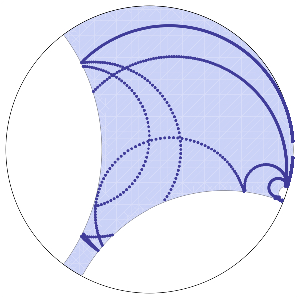
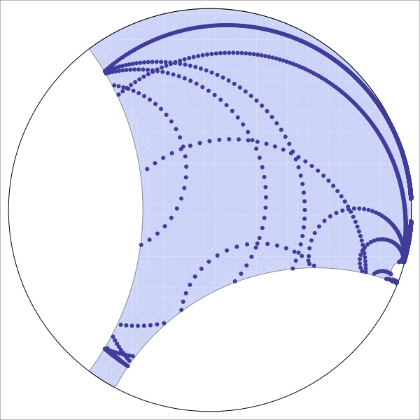
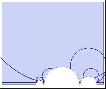
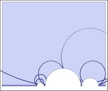
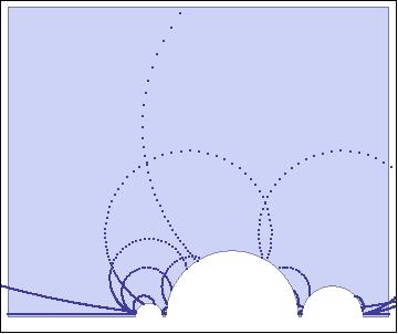
Figure 2. Equidistribution of expanding closed horocycles on a Schottky domain in the disk $\mathbb{D}$ and upper half plane $\mathbb{H}$ models.

Remark 1.12.

If $\Gamma$ is a lattice, then the closedness of $\Gamma\cap N\backslash N$ implies that $\Gamma\cap N\backslash N$ is compact. In this case, Sarnak [Sar81] proved the above result allowing $\psi\in C^{\infty}_{c}(\Gamma\backslash G)$ (that is, not requiring $K$-fixed), and with a best possible error term of

$$y^{\frac{1}{2}}$$

in place of our weaker bound

$$y^{{\frac{1}{2}}-\frac{3}{5}(\delta-{\frac{1}{2}})}.$$

1.4. Bounds for Automorphic Eigenfunctions

The proof of Theorem 1.11 requires control over the integrals of the eigenfunctions $\phi_{j}$, which a priori are only square-integrable. For the base eigenfunction, one has extra structure coming from Patterson theory [Pat76] which makes this control possible. But for the other eigenfunctions, this analysis fails. Nevertheless, the problem of obtaining such control was solved in the first-named author’s thesis [Kon07]. The statement is the following (see the Appendix as well).

Theorem 1.13 ([Kon07]).

Fix notation as in Theorem 1.11, and assume that the closed horocycle $(N\cap\Gamma)\backslash N$ is infinite. Let $\phi_{j}\in L^{2}(\Gamma\backslash\mathbb{H})$ be an eigenfunction of eigenvalue $\lambda_{j}=s_{j}(1-s_{j})<1/4$ with $s_{j}>1/2$. Then

$$\phi_{j}(n_{x}a_{y})\ll_{\phi_{j}}\left({y\over x^{2}+y^{2}}\right)^{s_{j}},$$

as $|x|\to\infty$ and $y\to 0$.

1.5. Organization of the Paper

In §2 we give some background and elaborate further on Theorem 1.5. For the reader’s convenience, in the Appendix we reproduce the proof of Theorem 1.13 from [Kon07], since this reference is not readily available. Equipped with such control, the proof of Theorem 1.11 follows with minor changes from the one given for one dimension higher in [KO08]. We sketch the argument in §3, and use it to prove Theorem 2.5 in §4. In §5, we verify the sieve axioms in Theorem 2.19 and conclude Theorem 2.23. At the end of §5, we derive the explicit values of $R$, in particular proving Theorem 1.5.

Acknowledgments.

The authors wish to express their gratitude to Peter Sarnak for many helpful discussions.

2. Background and More on Theorem 1.5

In this section, we elaborate on Theorem 1.5. Let $Q$ be a ternary rational quadratic form which is isotropic over $\mathbb{Q}$. Let $\Gamma<\operatorname{SO}_{Q}(\mathbb{Z})$ be a finitely generated subgroup with $\delta_{\Gamma}>1/2$.

As $Q$ is isotropic over $\mathbb{Q}$, we have a $\mathbb{Q}$-rational covering $\operatorname{SL}_{2}\to\operatorname{SO}_{Q}$. Therefore we may assume without loss of generality that $\Gamma$ is a finitely generated subgroup of $\operatorname{SL}_{2}(\mathbb{Z})$.

2.1. Uniform Spectral Gaps

For the application to sieving, Theorem 1.8 described in the introduction is insufficient. One requires uniformity along arithmetic progressions; hence we recall the notion of a spectral gap.

Let $\Gamma(q)$ denote the “congruence” subgroup of $\Gamma$ of level $q$,

$$\Gamma(q):=\{\gamma\in\Gamma:\gamma\equiv I(q)\}.$$

The inclusion of vector spaces

$$L^{2}(\Gamma\backslash\mathbb{H})\subset L^{2}(\Gamma(q)\backslash\mathbb{H})$$

induces the same inclusion on the spectral resolution of the Laplace operator:

$$\operatorname{Spec}(\Gamma\backslash\mathbb{H})\subset\operatorname{Spec}(\Gamma(q)\backslash\mathbb{H}).$$

Definition 2.1.

The new spectrum

$$\operatorname{Spec}_{new}(\Gamma(q)\backslash\mathbb{H})$$

at level $q$ is defined to be the set of eigenvalues below $1/4$ which are in $\operatorname{Spec}(\Gamma(q)\backslash\mathbb{H})$ but not in $\operatorname{Spec}(\Gamma\backslash\mathbb{H}).$

Definition 2.2.

A number $\theta$ in the interval $1/2<\theta<\delta$ is called a spectral gap for $\Gamma$ if there exists a ramification number $\mathfrak{B}\geq 1$ such that for any square-free

$$q=q^{\prime}q^{\prime\prime}\quad\text{ with }\quad q^{\prime}\mid\mathfrak{B}\text{ and }(q^{\prime\prime},\mathfrak{B})=1,$$

we have

$$\operatorname{Spec}(\Gamma(q)\backslash\mathbb{H})_{new}\cap(0,\theta(1-\theta))\quad\subset\quad\operatorname{Spec}(\Gamma(q^{\prime})\backslash\mathbb{H})_{new}.$$

That is, the eigenvalues below $\theta(1-\theta)$ which are new for $\Gamma(q)$ are coming from the “bad” part $q^{\prime}$ of $q$. As $\mathfrak{B}$ is a fixed integer depending only on $\Gamma$, there are only finitely many possibilities for its divisors $q^{\prime}$.

Collecting the results in [BG07, BGS08] and their extension from prime to square-free of [Gam02] we have:

Theorem 2.3 ([Gam02, BG07, BGS08]).

1. For any finitely generated $\Gamma<\operatorname{SO}_{Q}(\mathbb{Z})$ with critical exponent $\delta>1/2$, there exists some spectral gap

   $$1/2<\theta<\delta.$$

2. If $\delta>5/6$ then $\theta=5/6$ holds.

2.2. Counting with Weights uniformly in Level

Allowing some “smoothing”, one can count uniformly in cosets of orbits of level $q$ with explicit error terms. We fix a non-zero vector ${{\bf x}}_{0}\in\mathbb{Z}^{3}$ with $Q({{\bf x}}_{0})=0$ and set

$${\mathcal{O}}={{\bf x}}_{0}\Gamma.$$

We denote by $N_{0}$ the stabilizer subgroup of ${{\bf x}}_{0}$ in $G:=\operatorname{SL}_{2}(\mathbb{R})$. Then

$$N_{0}=g_{0}Ng_{0}^{-1}$$

for some $g_{0}\in\operatorname{SL}_{2}(\mathbb{Q})$, where $N$ denotes the upper triangular subgroup of $G$.

Set $K_{0}:=g_{0}\operatorname{SO}_{2}(\mathbb{R})g_{0}^{-1}$ and choose $\eta>0$ so that a $K_{0}$-invariant $\eta$ neighborhood $U_{\eta}$ of $e$ in $G$ injects to $\Gamma\backslash G$. Let $\psi:=\psi_{\eta}$ be a non-negative smooth $K_{0}$-invariant function on $G$ supported in $U_{\eta}$ with $\int\psi dg=1$.

Denote by $B_{T}$ a $K_{0}$-invariant norm ball in $\mathbb{R}^{3}$ about the origin with radius $T$.

Definition 2.4.

The weight $\xi_{T}:\mathbb{R}^{3}\to\mathbb{R}_{\geq 0}$ is defined as follows:

$$\xi_{T}({{\bf x}})=\int_{G}\chi_{T}({{\bf x}}g)\psi(g)dg$$

where $\chi_{T}$ denotes the characteristic function of $B_{T}$.

The sum of $\xi_{T}$ over ${\mathcal{O}}$ is precisely a smoothed count for $\#{\mathcal{O}}\cap B_{T}$ satisfying:

$$\sum_{{{\bf x}}\in{\mathcal{O}}}\xi_{T}({{\bf x}})\asymp\#{\mathcal{O}}\cap B_{T}.$$

Theorem 2.5.

Let $\theta$ be the spectral gap for $\Gamma$.

1. As $T\to\infty$,

   $$\Xi(T):=\sum_{{{\bf x}}\in{{\mathcal{O}}}}\xi_{T}({{\bf x}})\sim c\cdot T^{\delta},$$

   for some $c>0$.
   

2. For square-free $q$, write $q=q^{\prime}q^{\prime\prime}$ with $q^{\prime}\mid\mathfrak{B}$ and $(q^{\prime\prime},\mathfrak{B})=1$. Let $\Gamma_{1}(q)$ be any group satisfying

   $$\Gamma(q)\subset\Gamma_{1}(q)\subset\Gamma.$$

   Let $N_{0}$ be the stabilizer of ${{\bf x}}_{0}$ in $G$, and assume that

   $$\Gamma_{1}(q)\cap N_{0}=\Gamma\cap N_{0}.$$

   Fix any $\gamma_{0}\in\Gamma$ and $\varepsilon>0$. Then as $T\to\infty$,

   $$\sum_{{{\bf x}}\in{{\bf x}}_{0}\Gamma_{1}(q)}\xi_{T}({{\bf x}}\gamma_{0}) = {1\over[\Gamma:\Gamma_{1}(q)]}\cdot\bigg{(}\Xi(T)+\mathcal{E}(T,q^{\prime},\gamma_{0})\bigg{)}$$

   $$+O_{\varepsilon}\bigg{(}T^{\theta+\varepsilon}+T^{{\frac{1}{2}}+\frac{3}{5}(\delta-{\frac{1}{2}})+\varepsilon}\bigg{)},$$

   where the implied constant does not depend on $q$ or $\gamma_{0}$. Here the error term satisfies

   $$\mathcal{E}(T,q^{\prime},[\gamma_{0}])\ll T^{\delta-\zeta}$$

   for some fixed $\zeta>0$, does not depend on $q^{\prime\prime}$, and depends only on the class $[\gamma_{0}]$ in $\Gamma_{1}(q^{\prime})\backslash\Gamma$.

Remark 2.6.

Assuming that $\Gamma\cap N_{0}$ is a lattice in $N_{0}$, [Kon09] gives the above uniform count with the last error term

$$T^{{\frac{1}{2}}+\frac{3}{5}(\delta-{\frac{1}{2}})+\varepsilon}$$

replaced by a best possible error of

$$T^{{\frac{1}{2}}}\log T.$$

2.3. Zariski Density of Orbits of Pythagorean Triples

For simplicity, we will use the notation $\mathcal{P}(R)$ to denote the set of all integers having at most $R$ prime divisors.

Let ${{\bf x}}_{0}\in\mathbb{Z}^{3}$ be a non-zero Pythagorean triple on the cone

$$Q({{\bf x}})=x^{2}+y^{2}-z^{2}=0$$

and $\Gamma<\operatorname{SO}_{Q}(\mathbb{Z})$ a non-elementary finitely generated subgroup. Set

$${\mathcal{O}}:={{\bf x}}_{0}\cdot\Gamma.$$

Given a polynomial $F$ which is integral on ${\mathcal{O}}$, our goal is to find “small” values for $R=R({\mathcal{O}},F)$, for which $F$ “often” has at most $R$ prime factors.

In fact, when studying such thin orbits, the correct notion of “often” is not “infinitely often”, but instead one should require Zariski density. That is, the set of ${{\bf x}}\in{\mathcal{O}}$ for which $F({{\bf x}})\in\mathcal{P}(R)$ should not lie on a proper subvariety of the smallest variety containing ${\mathcal{O}}$. We illustrate this condition with the following examples.

2.3.1. Example I: Area

Recall that given any integral Pythagorean triple ${{\bf x}}=(x,y,z)$ which is also primitive (that is, there is no common divisor of $x$, $y$ and $z$), there exist coprime integers $u$ and $v$ of opposite parity (one even, one odd) such that, possibly after switching or negating $x$ and $y$, we have the ancient parametrization

$$x=u^{2}-v^{2},\quad y=2u\,v,\quad z=u^{2}+v^{2}.$$

In fact, this is just a restatement of the group homomorphism $\operatorname{SL}_{2}(\mathbb{R})\to\operatorname{SO}(2,1)$ given by

$$\left(\begin{array}[]{cc}a&b\\ c&d\end{array}\right)\mapsto\begin{pmatrix}{a^{2}-b^{2}-c^{2}+d^{2}\over 2}&{ac-bd}&{a^{2}-b^{2}+c^{2}-d^{2}\over 2}\\ {ab-cd}&{bc+ad}&{ab+cd}\\ {a^{2}+b^{2}-c^{2}-d^{2}\over 2}&{ac+bd}&{a^{2}+b^{2}+c^{2}+d^{2}\over 2}\end{pmatrix}$$

where $\operatorname{SL}(2,\mathbb{R})$ acts on $(u,v)$ and $\operatorname{SO}(2,1)$ acts on $(x,y,z)$.

Consider the “area” ${\frac{1}{2}}xy$ of the triple ${{\bf x}}$ (which may be negative). It is elementary that the area is always divisible by $6$, so the function

$$F_{\mathcal{A}}({{\bf x}}):={1\over 12}xy={1\over 6}(u+v)(u-v)u\,v$$ (2.7)

is integer-valued on ${\mathcal{O}}$.

Remark 2.8.

As above, we insist that the polynomial $F$ is integral on ${\mathcal{O}}$, but it need not necessarily have integer coefficients.

As (2.7) has four irreducible components, it is easy to show that there are only finitely many triples ${{\bf x}}$ for which $F_{\mathcal{A}}({{\bf x}})\in\mathcal{P}({2})$, that is, the product of at most two primes. Restricting to a subvariety such as

$$u=v+1,$$

it follows conjecturally from the Hardy-Littlewood $k$-tuple conjectures [HL22] that

$$\frac{1}{12}xy={1\over 6}(u+v)(u-v)u\,v={1\over 6}(2v+1)\cdot 1\cdot(v+1)\cdot v$$

will be the product of three primes for infinitely many $v$.

Since the set of triples generated in this way lies on a subvariety, it is not Zariski dense. On the other hand, it was recognized in [BGS08] that the recent work of Green and Tao [GT09] proves the infinitude and Zariski density of the set of all primitive Pythagorean triples ${{\bf x}}$ for which $F_{\mathcal{A}}({{\bf x}})\in\mathcal{P}({4})$, that is, has at most four prime factors.

Remark 2.9.

The results of Green-Tao do not apply to thin orbits, and neither do the conjectures of Hardy-Littlewood. Indeed, we conjecture that that if ${\mathcal{O}}$ is thin and $\Gamma$ has no unipotent elements (which would furnish an affine injection into ${\mathcal{O}}$), then there are only finitely-many points ${{\bf x}}$ for which $F_{\mathcal{A}}({{\bf x}})\in\mathcal{P}({3})$! On the other hand, allowing $4$ primes should lead to a Zariski dense set of triples ${{\bf x}}$. Below, we exhibit certain thin orbits for which there is a Zariski dense set of ${{\bf x}}$ with $F_{\mathcal{A}}({{\bf x}})\in\mathcal{P}(25)$.

Remark 2.10.

The critical number, $4,$ of prime factors above is related to the sieve dimension for this pair $({\mathcal{O}},F)$. We return to this issue shortly, cf. Remark 2.12.

2.3.2. Example II: Product of Coordinates

Consider now the product of coordinates $xyz$ for triples ${{\bf x}}\in{\mathcal{O}}$. It is elementary that $xyz$ is divisible by $60$, so the function

$$F_{\mathcal{C}}({{\bf x}}):={1\over 60}xyz={1\over 30}(u+v)(u-v)u\,v(u^{2}+v^{2})$$ (2.11)

is integer-valued.

$${1\over 60}xyz$$ has at most four prime factors

$${1\over 60}xyz$$ has exactly five prime factors

$${1\over 60}xyz$$ has six or more prime factors

Figure 3. The full orbit of all primitive Pythagorean triples.

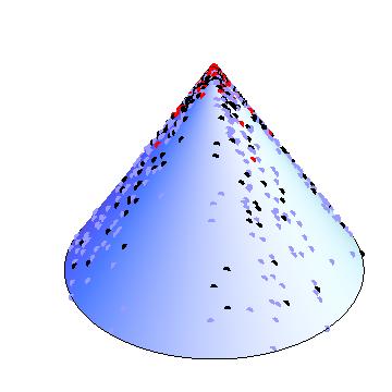
$${1\over 60}xyz$$ has at most four prime factors

$${1\over 60}xyz$$ has exactly five prime factors

$${1\over 60}xyz$$ has six or more prime factors

Figure 4. A thin orbit ${\mathcal{O}}$ of Pythagorean triples.

Now we note that as (2.11) has five irreducible components (and the sieve dimension is five). Therefore there are only finitely many triples ${{\bf x}}$ for which $F_{\mathcal{C}}({{\bf x}})\in\mathcal{P}(3)$. Restricting to a subvariety such as

$$u=v+3,$$

it follows conjecturally from Schinzel’s Hypothesis H [SS58] that

$${1\over 30}(u+v)(u-v)u\,v(u^{2}+v^{2})={1\over 30}(2v+3)\cdot(3)\cdot(v+3)\cdot v\cdot(2v^{2}+6v+9)$$

will be the product of four primes for infinitely many $v$. Again, this set is not Zariski dense in the cone. See Figure 3, where it is clear that such points frolic near the $x$ or $y$ axes.

On the other hand, it is a folklore conjecture that the set of triples ${{\bf x}}$ for which $F_{\mathcal{C}}({{\bf x}})\in\mathcal{P}(5)$ spreads out in every direction. For the full orbit of all primitive Pythagorean triples (rather than a thin one), the best known bound for the number of prime factors in $F_{\mathcal{C}}({{\bf x}})$ follows from the Diamond-Halberstam-Richert sieve [DHR88, DH97]. Their work shows that $F_{\mathcal{C}}({{\bf x}})\in\mathcal{P}(17)$ infinitely often.

Again, when the orbit ${\mathcal{O}}$ is thin without affine injections, we conjecture that there will be only finitely many ${{\bf x}}$ for which $F_{\mathcal{C}}({{\bf x}})\in\mathcal{P}(4)$ whereas five factors will be Zariski dense. Compare Figure 3 to Figure 4. We will exhibit certain thin orbits for which there is a Zariski dense set of ${{\bf x}}$ with $F_{\mathcal{C}}({{\bf x}})\in\mathcal{P}(29)$.

Remark 2.12.

Sieve dimension is not merely a function of the polynomial $F$ but really depends on the pair $({\mathcal{O}},F)$. In the related recent work [LS07], Liu and Sarnak consider $F_{\mathcal{C}}({{\bf x}})=xyz$, where the orbit ${\mathcal{O}}={{\bf x}}_{0}\cdot\Gamma$ is generated from a point ${{\bf x}}_{0}\in\mathbb{Z}^{3}$ on a one- or two-sheeted hyperboloid $Q({{\bf x}})=t$, where $t\neq 0$ and $Q$ is an indefinite integral ternary quadratic form which is anisotropic. Then the spin group of $G=\operatorname{SO}_{Q}(\mathbb{R})$ consists of the elements of norm one in a quaternion division algebra over $\mathbb{Q}$, and $\Gamma$ is the set of all such integral elements.

In particular, their orbit is full, whereas the focus of this paper is on thin orbits. A common feature, though, is that there do not exist non-constant polynomial parametrizations of points in ${\mathcal{O}}$ (in our case this corresponds precisely to $N_{0}\cap\Gamma$ being trivial).

The sieve dimension for Liu-Sarnak’s pair $({\mathcal{O}},F_{\mathcal{C}})$ is $3$ (whereas in our case, the same function $F=F_{\mathcal{C}}$ has sieve dimension $5$), and they prove the Zariski density of the set of points ${{\bf x}}\in{\mathcal{O}}$ for which $F_{\mathcal{C}}({{\bf x}})$ is in $\mathcal{P}(26)$. The precise definition of sieve dimension is given in Definition 2.16.

2.4. The Diamond-Halberstam-Richert Weighted Sieve

Let $\mathcal{A}=\{a_{n}\}$ be a sequence of non-negative real numbers, all but finitely many of which are zero.

For $R\geq 1$, let $\mathcal{P}(R)$ be the set of all integers having at most $R$ prime divisors counted with multiplicity. Let $\mathcal{W}=\{\omega(n)\}$ denote a certain sequence of weights supported on square-free numbers satisfying

$$\omega(n)\leq 0\quad\text{ if }\quad n\notin\mathcal{P}(R),$$ (2.13)

and being of convolution type, that is

$$\omega(n)=\sum_{d|n}\omega(d).$$ (2.14)

Let

$$S(\mathcal{A}\mathcal{W}):=\sum_{n}a_{n}\,\omega(n).$$

If we can construct a suitable sequence $\mathcal{W}$ with a good lower bound estimate for $S(\mathcal{A}\mathcal{W})$, then we can conclude by virtue of (2.13) that there are elements $a_{n}\in\mathcal{A}$ with $n\in\mathcal{P}(R)$, that is, having at most $R$ prime divisors.

Moreover, by (2.14) we can extract estimates for $S(\mathcal{A}\mathcal{W})$ from knowledge of the distribution of $\mathcal{A}$ along certain arithmetic progressions. For $q\geq 1$ a square-free integer, let

$$\mathcal{A}_{q}:=\{a_{n}\in\mathcal{A}:n\equiv 0(q)\}\quad\text{and}\quad|\mathcal{A}_{q}|:=\sum_{n\equiv 0(q)}a_{n},$$

so that

$$S(\mathcal{A}\mathcal{W})=\sum_{q}\omega(q)|\mathcal{A}_{q}|.$$

Assume there exists an approximation $\mathcal{X}$ to $|\mathcal{A}|:=\sum_{n}a_{n}$ and a non-negative multiplicative function $g(q)$ so that $g(q)\mathcal{X}$ is an approximation to $|\mathcal{A}_{q}|$. Assume that $g(1)=1$, $g(q)\in[0,1)$ for $q>1$, and that for constants $K\geq 2$, $\kappa\geq 1$ we have the local density bound

$$\prod_{{z_{1}\leq p\leq z}}(1-g(p))^{-1}\leq\left(\frac{\log z}{\log z_{1}}\right)^{\kappa}\left(1+{K\over\log z_{1}}\right)$$ (2.15)

for any $2\leq z_{1}<z$.

Definition 2.16.

The number $\kappa$ appearing in (2.15) is called the sieve dimension. (Note that it is not unique, as any larger value also satisfies (2.15); in practice one typically takes the least allowable value.)

We require that the remainder terms

$$r_{q}:=|\mathcal{A}_{q}|-g(q)\mathcal{X}$$

be small an average, that is, for some constants $\tau\in(0,1)$ and $A\geq 1$,

$$\sum_{q<\mathcal{X}^{\tau}(\log\mathcal{X})^{-A}\atop q\text{ squarefree}}4^{\nu(q)}|r_{q}|\ll{\mathcal{X}\over\log^{\kappa+1}\mathcal{X}}.$$ (2.17)

Finally, we introduce a parameter $\mu$ which controls the number of terms in $\mathcal{A}$ which are non-zero. Precisely, we require that

$$\max\{n\geq 1:a_{n}\neq 0\}\leq\mathcal{X}^{\tau\mu}.$$ (2.18)

We now state

Theorem 2.19 ([DHR88, DH97]).

Let $\mathcal{A}$, $z$, $\mathcal{X}$, $g$, $\kappa$, $\mu$ and $\tau$ be as described above.

1. Let $\sigma_{\kappa}(u)$ be the continuous solution of the differential-difference problem:

   $$\begin{cases}{u^{-\kappa}\sigma(u)=A_{\kappa}^{-1},}&\text{for $0<u\leq 2$, $A_{\kappa}=(2e^{\gamma})^{\kappa}\Gamma(\kappa+1)$,}\\ {(u^{-\kappa}\sigma(u))^{\prime}=-\kappa u^{-\kappa-1}\sigma(u-2),}&\text{for $u>2$,}\end{cases}$$ (2.20)

   where $\gamma$ is the Euler constant. Then there exist two numbers $\alpha_{\kappa}$ and $\beta_{\kappa}$ satisfying $\alpha_{\kappa}\geq\beta_{\kappa}\geq 2$ such that the following simultaneous differential-difference system has continuous solutions $F_{\kappa}(u)$ and $f_{\kappa}(u)$ which satisfy

   $$F_{\kappa}(u)=1+O(e^{-u}),\quad f_{\kappa}(u)=1+O(e^{-u}),$$

   and $F_{\kappa}$ (resp. $f_{\kappa}$) decreases (resp. increases) monotonically towards $1$ as $u\to\infty$:

   $$\begin{cases}{F(u)=1/\sigma_{\kappa}(u),}&\text{for $0<u\leq\alpha_{\kappa},$}\\ {f(u)=0,}&\text{for $0<u\leq\beta_{\kappa},$}\\ {(u^{\kappa}F(u))^{\prime}=\kappa u^{\kappa-1}f(u-1),}&\text{for $u>\alpha_{\kappa},$}\\ {(u^{\kappa}f(u))^{\prime}=\kappa u^{\kappa-1}F(u-1),}&\text{for $u>\alpha_{\kappa}.$}\end{cases}$$ (2.21)

2. For any two real numbers $u$ and $v$ with

   $$\tau^{-1}<u\leq v,\beta_{\kappa}<\tau v,$$

   there exist weights $\mathcal{W}=\{\omega(n)\}$ such that

   $$S(\mathcal{A}\mathcal{W})\gg\mathcal{X}\prod_{p<X^{1/v}}(1-g(p)),$$

   provided that

   $$R>\tau\mu u-1+{\kappa\over f_{\kappa}(\tau v)}\int_{1}^{v/u}F_{\kappa}(\tau v-s)\left(1-\frac{u}{v}s\right){ds\over s}.$$ (2.22)

2.5. Statement of the Main Theorem

The following is the main result of this paper.

Theorem 2.23.

Let $Q({{\bf x}})=x^{2}+y^{2}-z^{2}$, ${{\bf x}}_{0}\in\mathbb{Z}^{3}$ a non-zero vector with $Q({{\bf x}}_{0})=0$, and $\Gamma<\operatorname{SO}_{Q}(\mathbb{Z})$ a finitely generated subgroup with $\delta>1/2$. Denote by $\theta$ the spectral gap of $\Gamma$. Let $F$ be a polynomial which is integral on ${\mathcal{O}}$, such that the pair $({\mathcal{O}},F)$ is strongly primitive.

Then the following hold:

1. There are infinitely many ${{\bf x}}\in{\mathcal{O}}$ such that $F({{\bf x}})$ has at most $R$ prime factors, where $R({\mathcal{O}},F)$ is given by (2.22) with

   $$\tau<\min\left({\delta-\theta\over 2\delta},{\delta-{\frac{1}{2}}\over 5\delta}\right),\qquad\text{ and }\qquad\mu>\max\left({2\over\delta-\theta},{5\over\delta-1/2}\right).\\$$ (2.24)

2. Under the further assumption that $N_{0}\cap\Gamma$ is a lattice in $N_{0}$ for $N_{0}=\operatorname{Stab}_{G}({{\bf x}}_{0})$, the bounds in (2.24) improve to

   $$\tau<{\delta-\theta\over 2\delta},\qquad\text{ and }\qquad\mu>{2\over\delta-\theta}.$$ (2.25)

3. Denoting by $\kappa$ be the sieve dimension of $({\mathcal{O}},F)$,

   $$\#\{{{\bf x}}\in{\mathcal{O}}:\|{{\bf x}}\|<T,F({{\bf x}})\in\mathcal{P}(R)\}\asymp{T^{\delta}\over(\log T)^{\kappa}}.$$

   In particular, this set is Zariski dense in the cone $Q=0$.

2.6. Explicit Values of $R({\mathcal{O}},F)$

One must still work somewhat to obtain actual values of $R$ from Theorem 2.23. We now state the smallest values of $R({\mathcal{O}},F)$ which are achieved from Theorem 2.23, at the expense of requiring the critical exponent $\delta$ to be close to $1$.

The first statement we give is unconditional. Assuming $\delta>5/6$ and using Gamburd’s spectral gap $\theta=5/6$ from Theorem 2.3, the bounds (2.24) and (2.25) are equivalent. Hence assuming $N_{0}\cap\Gamma$ is a lattice in $N_{0}$ and using the optimal error terms in [Kon09] does not improve the final values of $R$. Said another way, the fact that our counting theorem is not optimal does not hurt the final values of $R$, unconditionally.

In the next three theorems, we keep the notation $Q,\Gamma,{\mathcal{O}}$ from Theorem 2.23. Let

$$F_{\mathcal{H}}({{\bf x}})=z,\qquad F_{\mathcal{A}}({{\bf x}})=\frac{1}{12}xy,\qquad F_{\mathcal{C}}({{\bf x}})=\frac{1}{60}xyz,$$

and assume the pair $({\mathcal{O}},F)$ is strongly primitive.

The following is the same as Theorem 1.5:

Theorem 2.26.

Let $\Gamma$ have critical exponent

$$\delta_{\mathcal{H}}>0.9992,\qquad\delta_{\mathcal{A}}>0.99995,\qquad\delta_{\mathcal{C}}>0.99677.$$

Then the proportion of ${{\bf x}}\in{\mathcal{O}}$ with $F({{\bf x}})\in\mathcal{P}(R)$ with $\|{{\bf x}}\|<T$ is

$$\asymp{1\over(\log T)^{\kappa}},$$

where

$$\kappa_{\mathcal{H}}=1,\qquad\kappa_{\mathcal{A}}=4,\qquad\kappa_{\mathcal{C}}=5,$$

and

$$\boxed{R_{\mathcal{H}}=14,\qquad R_{\mathcal{A}}=25,\qquad R_{\mathcal{C}}=29.}$$

We now observe the effect of the worse error term on the quality of $R({\mathcal{O}},F)$, conditioned on an improved spectral gap. Assuming $N_{0}\cap\Gamma$ is a lattice in $N_{0}$, the counting theorem in [Kon09] gives an optimal error term, which together with our sieve analysis gives the following.

Theorem 2.27.

Assume that $N_{0}\cap\Gamma$ is a lattice in $N_{0}$, and that the spectral gap $\theta$ can be arbitrarily close to $1/2$. Then if

$$\delta_{\mathcal{H}}>0.9265,\qquad\delta_{\mathcal{A}}>0.98805,\qquad\delta_{\mathcal{C}}>0.981675,$$

the conclusion of Theorem 2.26 holds with

$$\boxed{R_{\mathcal{H}}=6,\qquad R_{\mathcal{A}}=14,\qquad R_{\mathcal{C}}=17.}$$

Lastly, we demonstrate the values of $R$ which we can obtain without assuming that $\Gamma\cap N_{0}$ is a lattice in $N_{0}$.

Theorem 2.28.

We make no assumptions on $N_{0}\cap\Gamma$, but assume that $\theta$ can be arbitrarily close to $1/2$. Then if

$$\delta_{\mathcal{H}}>0.991,\qquad\delta_{\mathcal{A}}>0.97895,\qquad\delta_{\mathcal{C}}>0.99905,$$

the conclusion of Theorem 2.26 holds with

$$\boxed{R_{\mathcal{H}}=12,\qquad R_{\mathcal{A}}=23,\qquad R_{\mathcal{C}}=26.}$$

Theorems 2.26, 2.27, and 2.28 follow from Theorem 2.23 and Table 1, the computation of which is discussed in §5.3.

3. Equidistribution of Expanding Closed Horocycles

Let $G=\operatorname{SL}(2,\mathbb{R})$. We keep the notation for $N,A,K,n_{x},a_{y}$, etc., from (1.10). We have the Cartan decomposition

$$G=KA^{+}K$$

where $A^{+}:=\{a_{y}:0<y\leq 1\}$, as well as the Iwasawa decomposition $G=NAK$.

Let $\Gamma<G$ be a discrete finitely generated subgroup with critical exponent $\delta>1/2$. Assume the horocycle $(N\cap\Gamma)\backslash N$ is closed in $\Gamma\backslash G$. In this section, we prove Theorem 1.11.

3.1. Automorphic Representations and Spectral Bounds

Let $1/2<s<1$, and consider the character $\chi_{s}$ on the upper-triangular subgroup $B:=NA$ of $G$ defined by

$$\chi_{s}(na_{y})=y^{s}$$

where $a_{y}=\text{diag}(\sqrt{y},\sqrt{y}^{-1})$ is as before, and $n\in N$.

The unitarily induced representation $(\pi_{s}:=\operatorname{Ind}_{B}^{G}\chi_{s},V_{s})$ admits a unique $K$-invariant unit vector, say $v_{s}$.

By the theory of spherical functions,

$$f_{s}(g):=\langle\pi_{s}(g)v_{s},v_{s}\rangle=\int_{K}v_{s}(kg)dk$$

is the unique bi $K$-invariant function of $G$ with $f_{s}(e)=1$ and with $\mathcal{C}f_{s}=s(1-s)f_{s}$ where $\mathcal{C}$ is the Casimir operator of $G$. Moreover, there exist some $c_{s}>0$ and $\alpha>0$ such that for all $y$ small

$$f_{s}(a_{y})=c_{s}\cdot y^{1-s}(1+O(y^{\alpha}))$$

by [GV88, 4.6].

Since the Casimir operator is equal to the Laplace operator $\Delta$ on $K$-invariant functions, this immediately implies the following.

Theorem 3.1.

Let $\phi_{s}\in L^{2}(\Gamma\backslash G)^{K}\cap C^{\infty}(\Gamma\backslash G)$ satisfy $\Delta\phi_{s}=s(1-s)\phi_{s}$ and $\|\phi_{s}\|_{2}=1$. Then there exist $c_{s}>0$ and $\alpha>0$ such that for all $y\ll 1$,

$$\langle a_{y}\phi_{s},\phi_{s}\rangle_{L^{2}(\Gamma\backslash G)}=c_{s}\cdot y^{1-s}(1+O(y^{\alpha})).$$

The irreducible unitary representations of $G$ with $K$-fixed vector consist of principal series and the complimentary series. We use the parametrization of $s\in\{1/2+i\mathbb{R}\}\cup[1/2,1]$ so that the vertical line $1/2+i\mathbb{R}$ corresponds to the principal series and the complimentary series is parametrized by $1/2<s\leq 1$ with $s=1$ corresponding to the trivial representation.

Let $\{X_{1},X_{2},X_{3}\}$ denote an orthonormal basis of the (real) Lie algebra of $G$ with respect to an Ad-invariant scalar product. For $f\in C^{\infty}(\Gamma\backslash G)\cap L^{2}(\Gamma\backslash G)$, we consider the following Sobolev norm $\mathcal{S}_{m}(f)$:

$$\mathcal{S}_{m}(f)=\max\{\|X_{i_{1}}\cdots X_{i_{m}}(f)\|_{2}:1\leq i_{j}\leq 3\}.$$

The following is well-known (cf. [CHH88, Kna86]).

Proposition 3.2.

Let $(\pi,V)$ be a representation of $G$ which does not weakly contain any complementary series representation $V_{s}$. Then for any $\varepsilon>0$, and any smooth vectors $v_{1},v_{2}\in V$,

$$|\langle\pi(a_{y})v_{1},v_{2}\rangle|\ll_{\varepsilon}y^{1/2-\varepsilon}\cdot\|\mathcal{S}_{1}(v_{1})\|\cdot\|\mathcal{S}_{1}(v_{2})\|,\qquad\text{ as }\qquad y\to 0.$$

3.2. Approximations to Integrals over closed horocycles

As $\delta>1/2$, there exists a unique positive $L^{2}$-eigenfunction $\phi_{0}$ of the Laplace operator $\Delta=-y^{2}\left(\partial_{xx}+\partial_{yy}\right)$ on $\Gamma\backslash\mathbb{H}$ with smallest eigenvalue $\delta(1-\delta)$ and of unit norm [Pat76]. The spectrum of $\Delta$ acting on $L^{2}(\Gamma\backslash\mathbb{H})$ has finitely many discrete points below $1/4$ and is purely continuous above $1/4$ [LP82].

Order the other discrete eigenvalues $\lambda_{j}=s_{j}(1-s_{j})$, with $s_{j}>1/2$, $j=1,\dots,k$ and let $\phi_{j}$ denote the corresponding eigenfunction with $\|\phi_{j}\|=1$. For uniformity of notation, set $s_{0}:=\delta$.

The map $g\mapsto g(i)$ gives an identification of $G/K$ with $\mathbb{H}$. Below a $K$-invariant function $\phi$ of $G$ may be considered as a function on the upper half plane $\mathbb{H}$ by $\phi(x+iy):=\phi(n_{x}a_{y})$ and vice versa.

Let $dg$ denote the Haar measure of $G$ given by

$$d(n_{x}a_{y}k)=y^{-2}dxdydk$$

where $dk$ is the probability Haar measure on $K$, and $dx$ and $dy$ are Lebesque measures. Hence for $\psi_{1},\psi_{2}\in L^{2}(\Gamma\backslash G)^{K}$,

$$\left\langle\psi_{1},\psi_{2}\right\rangle=\int_{\Gamma\backslash G}\psi_{1}(g)\overline{\psi_{2}(g)}\;dg=\int_{\Gamma\backslash\mathbb{H}}\psi_{1}(x+iy)\overline{\psi_{2}(x+iy)}\;dx\frac{dy}{y^{2}}.$$

Proposition 3.3.

For any smooth $\psi_{1}\in L^{2}(\Gamma\backslash G)^{K}$ and $\psi_{2}\in C_{c}^{\infty}(\Gamma\backslash G)$,

$$\langle a_{y}\psi_{1},\psi_{2}\rangle =\sum_{j=0}^{k}\langle\psi_{1},\phi_{j}\rangle\langle a_{y}\phi_{j},\psi_{2}\rangle+O_{\varepsilon}(y^{1/2-\varepsilon}\mathcal{S}_{1}(\psi_{1})\cdot\mathcal{S}_{1}(\psi_{2})).$$

as $y\to 0$.

Proof.

Write

$$L^{2}(\Gamma\backslash G)=W_{\lambda_{0}}\oplus\cdots\oplus W_{\lambda_{k}}\oplus V$$

where $W_{\lambda_{j}}$ is isomorphic as a $G$-representation to the complementary series representation $V_{s_{j}}$, $\lambda_{j}=s_{j}(1-s_{j})$, and $V$ is tempered. Write

$$\psi_{1}=\langle\psi_{1},\phi_{0}\rangle\phi_{0}+\dots+\langle\psi_{1},\phi_{k}\rangle\phi_{k}+\psi_{1}^{\perp}.$$

Since the $\phi_{j}$’s are the unique $K$-invariant vectors in $W_{\lambda_{j}}$ (up to scalar), we have $\psi_{1}^{\perp}\in V^{K}$. Hence by Proposition 3.2, for any $\varepsilon>0$ and $y\ll 1$,

$$\langle a_{y}\psi_{1},\psi_{2}\rangle =\sum_{j=0}^{k}\langle\psi_{1},\phi_{j}\rangle\langle a_{y}\phi_{j},\psi_{2}\rangle+\langle a_{y}\psi_{1}^{\perp},\psi_{2}\rangle$$

$$=\sum_{j=0}^{k}\langle\psi_{1},\phi_{j}\rangle\langle a_{y}\phi_{j},\psi_{2}\rangle+O_{\varepsilon}(y^{1/2-\varepsilon}\mathcal{S}_{1}(\psi_{1})\cdot\mathcal{S}_{1}(\psi_{2}))$$

since $\mathcal{S}_{1}(\psi_{1}^{\perp})\ll\mathcal{S}_{1}(\psi_{1})$. ∎

The main goal of this subsection is to study the averages of the $\phi_{j}$’s along the translates $(N\cap\Gamma)\backslash Na_{y}$.

We first need to recall some geometric facts. The limit set $\Lambda(\Gamma)$ of $\Gamma$ is the set of all accumulation points of an orbit $\Gamma(z_{0})$ for some $z_{0}\in\mathbb{H}$. As $\Gamma$ is discrete, it easily follows that $\Lambda(\Gamma)$ is a subset of $\partial_{\infty}(\mathbb{H})=\mathbb{R}\cup\{\infty\}$.

Geometrically, $N(i)\subset\mathbb{H}$ is a horocycle based at $\infty$. Since $\Gamma$ is finitely generated, the closedness of its projection to $\Gamma\backslash\mathbb{H}$ implies either that $\infty$ is a parabolic fixed point, that is, $N\cap\Gamma$ is non-trivial, or that $\infty$ lies outside the limit set $\Lambda(\Gamma)$ [Dal00].

We define for each $0\leq j\leq k$

$$\phi_{j}^{N}(a_{y}):=\int_{\Gamma\cap N\backslash N}\phi_{j}(na_{y})dn.$$ (3.4)

Theorem 3.5.

For any $j=0,\dots,k$, the integrals in (3.4) converge absolutely. Moreover there exist constants $c_{j}$ and $d_{j}$, depending on $\phi_{j}$, such that

$$\phi_{j}^{N}(a_{y})=c_{j}y^{1-s_{j}}+d_{j}y^{s_{j}}.$$

Furthermore, $c_{0}>0$.

Proof.

We first establish the convergence of the integral in (3.4). If $\infty$ is a parabolic fixed point, that is, if $N\cap\Gamma$ is a lattice in $N$, then the domain of this integral is finite, and of course the eigenfunctions of the Laplace operator are bounded, so we are done.

On the other hand, if $\infty\notin\Lambda(\Gamma)$, then Theorem A.1 applies, that for $y$ fixed,

$$\phi_{j}(n_{x}a_{y})\ll_{y}(1+x^{2})^{-s_{j}}.$$

Then the integral $\int_{-\infty}^{\infty}\phi_{j}(n_{x}a_{y})dx$ clearly converges, since $s_{j}>1/2$.

Since

$$\Delta\phi_{j}=s_{j}(1-s_{j})\phi_{j},$$

it follows that

$$-y^{2}\frac{\partial^{2}}{\partial y^{2}}\phi_{j}^{N}=s_{j}(1-s_{j})\phi_{j}^{N}.$$

The two independent solutions to this equation are $y^{s_{j}}$ and $y^{1-s_{j}}$.

Lastly, we must demonstrate that $c_{0}>0$. If $\infty\notin\Lambda(\Gamma)$, this is done as in [Kon07] (see also [KO08, Equation (4.11)]), by proving explicitly that

$$\phi_{0}^{N}(a_{y})=c_{0}\ y^{1-\delta},$$

i.e. $d_{0}=0$. As $\phi_{0}$ is a positive function, this implies $c_{0}>0$.

If on the other hand $\infty$ is a parabolic fixed point for $\Gamma$, then as the Dirichlet domain for $\Gamma$ is a finite sided polygon with $\infty$ as a vertex [Bea83], it follows that for some $Y_{0}\gg 1$, $(N\cap\Gamma)\backslash N\times[Y_{0},\infty)$ injects to $\Gamma\backslash\mathbb{H}$. Therefore, if we had $c_{0}=0$ and hence $\phi_{0}(n_{x}a_{y})=d_{0}y^{\delta_{\Gamma}}$, then

$$1=\|\phi_{0}\|^{2}\geq\int_{Y_{0}}^{\infty}\int\limits_{n_{x}\in(N\cap\Gamma)\backslash N}|\phi_{0}(n_{x}a_{y})|^{2}d{x}\frac{dy}{y^{2}}\\ \geq\int_{(N\cap\Gamma)\backslash N}1\;dn\cdot\int_{Y_{0}}^{\infty}d_{0}^{2}y^{2\delta-2}{dy}=\infty,$$

since $\delta>1/2$.

This contradiction gives the desired result. ∎

The following Proposition shows that to compute $\phi_{j}^{N}$, it suffices to integrate over a bounded set $J$; the error term, if any, is small.

If $N\cap\Gamma$ is a lattice in $N$, set $J:=(N\cap\Gamma)\backslash N$. Otherwise as $\infty\notin\Lambda(\Gamma)$, $\Lambda(\Gamma)$ is a compact subset of $\mathbb{R}$, and we let $J\subset(N\cap\Gamma)\backslash N=\mathbb{R}$ be an open bounded interval which contains $\Lambda(\Gamma)$. In either case $J$ is a bounded interval.

Proposition 3.6.

We have

$$\phi_{j}^{N}(a_{y})=\int_{J}\phi_{j}(n_{x}a_{y})\;dx+O(y^{s_{j}}),$$ (3.7)

as $y\to 0$.

Proof.

If $N\cap\Gamma$ is a lattice in $N$, then $\phi_{j}^{N}$ and $\int_{J}\phi_{j}$ are identical; there is nothing to prove. Otherwise, denoting by $J^{c}$ the complement of $J$, we have

$$\int_{n_{x}\in J^{c}}\phi_{j}(n_{x}a_{y})dn_{x}\ll y^{s_{j}}.$$

by Theorem A.1, which completes the proof. ∎

Next, we approximate $\phi_{j}^{N}$ by smoothing further in a transverse direction. Denote by $U_{\epsilon}$ the ball of radius $\epsilon$ about $e$ in $G$. Let $J$ be as in Proposition 3.6.

Denoting by $N^{-}$ the lower triangular subgroup of $G$, we note that $NAN^{-}$ forms an open dense neighborhood of $e$ in $G$.

Definition 3.8.

• We fix a non-negative function $\eta\in C_{c}^{\infty}(\Gamma\cap N\backslash N)$ with $\eta=1$ on $J$.

• Let $U_{c_{0}}$ denote the $c_{0}$-neighborhood of the identity $e$, and fix $c_{0}>0$ so that the multiplication map

  $$\operatorname{supp}(\eta)\times(U_{c_{0}}\cap AN^{-})\to\operatorname{supp}(\eta)(U_{c_{0}}\cap AN^{-})\subset\Gamma\backslash G$$

  is a bijection onto its image.

• For each $\epsilon<c_{0}$, let $r_{\epsilon}$ be a non-negative smooth function in $AN^{-}$ whose support is contained in

  $$W_{\epsilon}:=(U_{\epsilon}\cap A)(U_{c_{0}}\cap N^{-})$$

  and $\int_{W_{\epsilon}}r_{\epsilon}\;d\nu=1$.

• We define the following function $\rho_{\eta,\epsilon}$ on $\Gamma\backslash G$ which is $0$ outside $\operatorname{supp}(\eta)U_{c_{0}}$, and for $g=n_{x}an^{-}\in\operatorname{supp}(\eta)(U_{c_{0}}\cap AN^{-})$,

  $$\rho_{\eta,\epsilon}(g):=\eta(n_{x})\otimes r_{\epsilon}(an^{-}).$$

Proposition 3.9.

We have for all small $0<\epsilon\ll\epsilon_{0}$ and for all $0<y<1$,

$$|\phi_{j}^{N}(a_{y})-\langle a_{y}\phi_{j},\rho_{\eta,\epsilon}\rangle_{L^{2}(\Gamma\backslash G)}|\ll\epsilon\cdot y^{1-s_{j}}.$$

Proof.

This follows in the same way as Proposition 6.4 in [KO08]. ∎

The next corollary follows immediately from Proposition 3.9 and Theorem 3.5.

Corollary 3.10.

For $\epsilon<1$, and $j=0,1,\dots,k$,

$$\langle a_{y}\phi_{j},\rho_{\eta,\epsilon}\rangle_{L^{2}(\Gamma\backslash G)}\ll y^{1-s_{j}},$$

as $y\to 0$.

3.3. Proof of Theorem 1.11

The proof is almost identical to the proof of Theorem 6.1 in [KO08]. We sketch the main steps.

We use the following lemma, which is standard in Sobolev theory.

Lemma 3.11.

For $\psi\in C^{\infty}_{c}(\Gamma\backslash G)^{K}$, there exists $\psi^{\sharp}\in C^{\infty}_{c}(\Gamma\backslash G)^{K}$ such that

1. for any $\epsilon<\epsilon_{0}$ and $h\in U_{\epsilon}$,

   $$|\psi(g)-\psi(gh)|\leq\epsilon\cdot\psi^{\sharp}(g)\quad\text{ for all $g\in\Gamma\backslash G$}.$$

2. $\mathcal{S}_{m}(\psi^{\sharp})\ll\mathcal{S}_{m+1}(\psi)$ for each $m\in\mathbb{N}$, where the implied constant depends only on $\operatorname{supp}(\psi)$.

Definition 3.12.

For a given $\psi\in C^{\infty}(\Gamma\backslash G)^{K}$ and $\eta\in C_{c}(\Gamma\cap N\backslash N)$, define the function $\mathcal{I}_{\eta}(\psi)$ on $G$ by

$$\mathcal{I}_{\eta}(\psi)(a_{y}):=\int_{n\in(\Gamma\cap N)\backslash N}\psi(na_{y})\eta(n)\;dn.$$

Proposition 3.13.

Let $\psi\in C^{\infty}(\Gamma\backslash G)^{K}$. Then for any $0<y<1$ and any small $\epsilon>0$,

$$|\mathcal{I}_{\eta}(\psi)(a_{y})-\langle a_{y}\psi,\rho_{\eta,\epsilon}\rangle|\ll(\epsilon+y)\cdot\mathcal{I}_{\eta}(\psi^{\sharp})(a_{y}),$$

where $\psi^{\sharp}$ is given by Lemma 3.11.

Proof.

This is the same as Proposition 6.6 in [KO08]. ∎

By Proposition 3.6, we have that

$$\phi_{j}^{N}(a_{y})=\mathcal{I}_{\eta}(\phi_{j})(a_{y})+O(y^{s_{j}}).$$

For simplicity, we set $\rho_{\epsilon}=\rho_{\eta,\epsilon}$ where $\rho_{\eta,\epsilon}=\eta\otimes r_{\epsilon}$ is defined as in Def. 3.8. Noting that $r_{\epsilon}$ is essentially an $\epsilon$-approximation only in the $A$-direction, we obtain that $\mathcal{S}_{1}(\rho_{\epsilon})=O(\epsilon^{-3/2})$.

Set $p=3/2$. Fix $\ell$, a parameter to be chosen later. Setting $\psi_{0}(g):=\psi(g)$, we define for $1\leq i\leq\ell$, inductively

$$\psi_{i}(g):=\psi_{i-1}^{\sharp}(g)$$

where $\psi_{i-1}^{\sharp}$ is given by Lemma 3.11.

Applying Proposition 3.13 to each $\psi_{i}$, we obtain for $0\leq i\leq\ell-1$

$$\mathcal{I}_{\eta}(\psi_{i})(a_{y})=\langle a_{y}\psi_{i},\rho_{\epsilon}\rangle+O((\epsilon+y)\mathcal{I}_{\eta}(\psi_{i+1})(a_{y}))$$

and

$$\mathcal{I}_{\eta}(\psi_{\ell})(a_{y})=\langle a_{y}\psi_{\ell},\rho_{\epsilon}\rangle+O((\epsilon+y)\mathcal{S}_{1}({\psi_{\ell}})).$$

Note that by Corollary 3.3, we have for each $1\leq i\leq\ell$

$$\langle a_{y}\psi_{i},\rho_{\epsilon}\rangle =\sum_{j=0}^{k}\langle\psi_{i},\phi_{j}\rangle\langle a_{y}\phi_{j},\rho_{\epsilon}\rangle+O(y^{1/2}\mathcal{S}_{1}(\rho_{\epsilon}))$$

$$\ll_{\psi}y^{1-\delta}.$$

Combining the above with Proposition 3.9 and Corollary 3.10, we get that for any $y<\epsilon$,

$$\mathcal{I}_{\eta}(\psi)(a_{y}) = \langle a_{y}\psi,\rho_{\epsilon}\rangle+O\left(\sum_{i=1}^{\ell-1}\langle a_{y}\psi_{i},\rho_{\epsilon}\rangle(\epsilon+y)^{k}\right)+O(\mathcal{S}_{\ell+1}(\psi)(\epsilon+y)^{\ell})$$

$$= \sum_{j=0}^{k}\langle\psi,\phi_{j}\rangle\langle a_{y}\phi_{j},\rho_{\epsilon}\rangle+O(y^{1/2}\mathcal{S}_{1}(\rho_{\epsilon}))+O\left(\sum_{i=1}^{\ell-1}y^{1-\delta}\epsilon^{k}\right)+O(\epsilon^{\ell})$$

$$= \sum_{j=0}^{k}\langle\psi,\phi_{j}\rangle\phi_{j}^{N}(a_{y})+O\left(\epsilon\cdot y^{1-\delta}\right)+O_{\varepsilon}(y^{1/2-\varepsilon}\epsilon^{-p})+O(\epsilon^{\ell}),$$

where the implied constants depend on the Sobolev norms of $\psi$. Balancing the first two error terms and recalling $p=3/2$, one arrives at the optimal choice

$$\epsilon=y^{(\delta-1/2)/(1+p)}.$$

With this choice of $\epsilon$, the first two error terms are $\ll_{\varepsilon}y^{{4-3\delta\over 5}-\varepsilon}$. Lastly, we choose $\ell$ to make the final error term of the same quality, namely $\ell=(4-3\delta)/(2\delta-1).$

Therefore

$$\int_{(N\cap\Gamma)\backslash N}\psi(na_{y})\;dn=\sum_{j=0}^{k}\langle\psi,\phi_{j}\rangle\phi_{j}^{N}(a_{y})+O_{\psi,\varepsilon}(y^{{4-3\delta\over 5}-\varepsilon}),$$

for any $\varepsilon>0$.

This completes the proof of Theorem 1.11.

4. Proofs of the Counting Theorems

With Theorem 1.11 at hand, we now count establish the counting theorems; these are Theorems 1.8 and 2.5.

4.1. Proof of Theorem 1.8

Recall that $Q$ is a ternary indefinite quadratic form, $\operatorname{SO}_{Q}(\mathbb{R})$, and $\Gamma$ a finitely generated discrete subgroup with $\delta_{\Gamma}>1/2$. Fix a non-zero vector ${{\bf x}}_{0}\in\mathbb{R}^{3}$, lying on the cone $Q=0$ such that the orbit ${\mathcal{O}}={{\bf x}}_{0}\Gamma$ is discrete.

Let

$$\mathcal{N}(T):=\#\{{{\bf x}}\in{\mathcal{O}}:\|{{\bf x}}\|<T\}$$

where $\|\cdot\|$ denotes a Euclidean norm on $\mathbb{R}^{3}$.

Using the spin cover $\iota:\operatorname{SL}_{2}\to\operatorname{SO}_{Q}$, we may assume without loss of generality that $\Gamma$ is a finitely generated subgroup of $G:=\operatorname{SL}_{2}(\mathbb{R})$ with $\delta_{\Gamma}>1/2$. We use the notation $N,A,K,a_{y},n_{x}$, etc from the introduction. Let $dg$ denote the Haar measure given by

$$d(n_{x}a_{y}k)=y^{-2}dxdydk$$

where $dk$ is the probability Haar measure on $K$, and $dx$ and $dy$ are Lebesque measures.

As $Q({{\bf x}}_{0})=0$, the stabilizer of ${{\bf x}}_{0}$ in $G$ is conjugate to $N$ and hence by replacing $\Gamma$ with a conjugate if necessary, we may assume without loss of generality that $N$ is precisely the stabilizer subgroup of ${{\bf x}}_{0}$ in $G$. It follows that ${{\bf x}}_{0}a_{y}=y^{-1}{{\bf x}}_{0}$. Let $B_{T}$ be a $K$-invariant ball of radius $T$ in $\mathbb{R}^{3}$, and let $\chi_{T}$ be the characteristic function of this ball. Note that $\chi_{T}$ is right $K$-invariant, that is, $\chi_{T}({{\bf x}}gk)=\chi_{T}({{\bf x}}g)$, for any $g\in G$ and $k\in K$. Also, as $N$ is the stabilizer of ${{\bf x}}_{0}$, we have $\chi_{T}({{\bf x}}_{0}ng)=\chi_{T}({{\bf x}}_{0}g)$, for any $n\in N$, that is, $\chi_{T}$ is left $N$-invariant.

We define the following counting function on $\Gamma\backslash G$:

$$F_{T}(g):=\sum_{\gamma\in N\cap\Gamma\backslash\Gamma}\chi_{T}({{\bf x}}_{0}\gamma g).$$

Lemma 4.1.

For any $\Psi\in C_{c}(\Gamma\backslash G)^{K}$,

$$\langle F_{T},\Psi\rangle=\int_{y>T^{-1}\|{{\bf x}}_{0}\|}\int_{n_{x}\in\Gamma\cap N\backslash N}\Psi(n_{x}a_{y})y^{-2}dxdy.$$

Proof.

We observe that by unfolding and using the $K$-invariance of $\Psi$ and $\chi_{B_{T}}$,

$$\langle F_{T},\Psi\rangle =\int_{\Gamma\backslash G}\sum_{\Gamma\cap N\backslash\Gamma}\chi_{B_{T}}({{\bf x}}_{0}\gamma g)\Psi(g)dg$$

$$=\int_{\Gamma\cap N\backslash G}\chi_{B_{T}}({{\bf x}}_{0}g)\Psi(g)dg$$

$$=\int_{\|{{\bf x}}_{0}a_{y}\|<T}\int_{\Gamma\cap N\backslash N}\Psi(na_{y})y^{-2}dndy.$$

As ${{\bf x}}_{0}a_{y}=y^{-1}{{\bf x}}_{0}$, the claim follows. ∎

As before, we order discrete eigenvalues $0\leq\lambda_{0}<\lambda_{1}\leq\lambda_{2}\cdots\leq\lambda_{k}<1/4$ of $\Delta$ on $L^{2}(\Gamma\backslash\mathbb{H})$ with $\lambda_{j}=s_{j}(1-s_{j})$, with $s_{j}>1/2$, $j=1,\dots,k$ and let $\phi_{j}\in L^{2}(\Gamma\backslash\mathbb{H})$ denote the corresponding eigenfunction with $\|\phi_{j}\|=1$.

Recall by Theorem 3.5, there exist constants $c_{j}$ and $d_{j}$, depending on $\phi_{j}$, such that

$$\phi_{j}^{N}(a_{y})=c_{j}y^{1-s_{j}}+d_{j}y^{s_{j}}.$$

Furthermore, $c_{0}>0$.

By inserting the asymptotic formula for $\int_{\Gamma\cap N\backslash N}\Psi(na_{y})dn$ from Theorem 1.11, we deduce:

Proposition 4.2.

For any $\Psi\in C_{c}^{\infty}(\Gamma\backslash G)^{K}$ and $\epsilon>0$,

$$\left\langle F_{T},\Psi\right\rangle_{\Gamma\backslash G} =\sum_{j=0}^{k}\left\langle F_{T},\phi_{j}\right\rangle_{\Gamma\backslash G}\left\langle\Psi,\phi_{j}\right\rangle_{\Gamma\backslash G}+O_{\varepsilon}\bigg{(}T^{{\frac{1}{2}}+\frac{3}{5}(\delta-{\frac{1}{2}})+\varepsilon}\bigg{)}$$

$$=\sum_{j=0}^{k}\langle\Psi,\phi_{j}\rangle_{\Gamma\backslash G}\left(\frac{c_{j}T^{s_{j}}}{s_{j}\|{{\bf x}}_{0}\|^{s_{j}}}+\frac{d_{j}T^{1-s_{j}}}{(1-s_{j})\|{{\bf x}}_{0}\|^{1-s_{j}}}\right)+O_{\epsilon}(T^{\frac{1}{2}+\frac{3}{5}(\delta-\frac{1}{2})+\epsilon})$$

where the implied constant depends only on a Sobolev norm of $\Psi$ and $\epsilon$.

For all small $\eta>0$, consider an $\eta$-neighborhood $U_{\eta}$ of $e$ in $G$, which is $K$-invariant, such that for all $T\gg 1$,

$$B_{T}U_{\eta}\subset B_{(1+\eta)T}\quad\text{and}\quad B_{(1-\eta)T}\subset\cap_{u\in U_{\eta}}B_{T}u.$$

Let $\psi_{\eta}\in C^{\infty}(\mathbb{H})$ denote a non-negative function supported on $U_{\eta}$ with $\int_{G}\psi dg=1$. We lift $\psi_{\eta}$ to $\Gamma\backslash G$ by

$$\Psi_{\eta}(g):=\sum_{\gamma\in\Gamma}\psi_{\eta}(\gamma g).$$

Then

$$\langle F_{(1-\eta)T},\Psi_{\eta}\rangle\leq F_{T}(e)\leq\langle F_{(1+\eta)T},\Psi_{\eta}\rangle.$$ (4.3)

On the other hand, recalling that $\{X_{1},X_{2},X_{3}\}$ is an orthonormal basis for the Lie algebra $\mathfrak{g}=\mathfrak{s}l(2,\mathbb{R})$ of $G$, we have

$$\langle\Psi_{\eta},\phi_{j}\rangle=\phi_{j}(e)+O(\eta\sup_{g\in U_{\eta}}\sup_{i=1,2,3}X_{i}\phi_{j}(g))$$

where the implied constant is absolute.

Therefore Proposition 4.2 yields for $C_{0}=\frac{\phi_{0}(e)c_{0}}{\delta\|{{\bf x}}_{0}\|^{\delta}}>0$,

$$\langle F_{(1-\eta)T},\Psi_{\eta}\rangle=C_{0}T^{\delta}+O_{\epsilon}(T^{s_{1}}+\eta T^{\delta}+\eta^{-A}T^{\frac{1}{2}+\frac{3}{5}(\delta-\frac{1}{2})+\epsilon})$$

for some $A>0$ and any $\epsilon>0$, where we used that the Sobolev norms of $\Psi_{\eta}$ grow at most polynomially in $\eta$; the implied constant now depends only on $\epsilon$. Therefore by equating the last two terms, we can choose $\eta=T^{-r}$ for some $r>0$ and obtain from (4.3) that

$$F_{T}(e)=C_{0}T^{\delta}+O(T^{\delta-\zeta})$$

for some $\zeta>0$. This proves Theorem 1.8.

4.2. Proof of Theorem 2.5:

As in the discussion preceding Theorem 2.5, we may assume that $\Gamma$ is a finitely generated subgroup of $\operatorname{SL}_{2}(\mathbb{Z})$. We may also assume without loss of generality that $g_{0}=e$ by replacing $\Gamma$ by $g_{0}\Gamma g_{0}^{-1}$ and hence the stabilizer subgroup of ${{\bf x}}_{0}$ in $G$ is precisely the upper triangular subgroup $N$. Recall the weight $\xi_{T}$ defined in Definition 2.4.

Let $q\geq 1$ be squarefree, and let $\Gamma_{1}(q)$ be any group satisfying

$$\Gamma(q)\subset\Gamma_{1}(q)\subset\Gamma$$

and

$$N\cap\Gamma_{1}(q)=N\cap\Gamma,$$ (4.4)

where $\Gamma(q)=\{\gamma\in\Gamma:\gamma\equiv I(q)\}$ is the “congruence” subgroup of $\Gamma$ of level $q$.

We define the following $K$-invariant functions on $\Gamma_{1}(q)\backslash G$:

$$F_{T}^{q}(g):=\sum_{\gamma\in(N\cap\Gamma)\backslash\Gamma_{1}(q)}\chi_{T}({{\bf x}}_{0}\gamma g),$$

and for any fixed $\gamma_{0}\in\Gamma$,

$$\Psi_{\gamma_{0}}^{q}(g):=\sum_{\gamma\in\Gamma_{1}(q)}\psi(\gamma_{0}^{-1}\gamma g).$$

Proposition 4.5.

We have

$$\sum_{{{\bf x}}\in{{\bf x}}_{0}\Gamma_{1}(q)}\xi_{T}({{\bf x}}\gamma_{0})=\left\langle F_{T}^{q},\Psi_{\gamma_{0}}^{q}\right\rangle_{\Gamma_{1}(q)\backslash G}.$$ (4.6)

Proof.

Starting with the left hand side of (4.6), we insert Definition 2.4, use that $N$ stabilizes ${{\bf x}}_{0}$, and that $N\cap\Gamma=N\cap\Gamma_{1}(q)$:

$$\sum_{{{\bf x}}\in{{\bf x}}_{0}\Gamma_{1}(q)}\xi_{T}({{\bf x}}\gamma_{0}) = \sum_{{{\bf x}}\in{{\bf x}}_{0}\Gamma_{1}(q)}\int_{G}\chi_{T}({{\bf x}}\gamma_{0}g)\psi(g)dg$$

$$= \sum_{\gamma\in(N\cap\Gamma)\backslash\Gamma_{1}(q)}\int_{G}\chi_{T}({{\bf x}}_{0}\gamma g)\psi(\gamma_{0}^{-1}g)dg$$

$$= \int_{G}F_{T}^{q}(g)\psi(\gamma_{0}^{-1}g)dg$$

$$= \sum_{\gamma\in\Gamma_{1}(q)}\int_{\Gamma_{1}(q)\backslash G}F_{T}^{q}(g)\psi(\gamma_{0}^{-1}\gamma g)dg$$

$$= \int_{G}F_{T}^{q}(g)\Psi_{\gamma_{0}}(g)dg,$$

where we used the definition of $F_{T}^{q}$, “refolded” (the reverse of the “unfolding trick”), and used the definition of $\Psi_{\gamma_{0}}^{q}$. ∎

Applying Proposition 4.2 to each $\Gamma_{1}(q)$ and noting that Sobolev norms of $\Psi_{\gamma_{0}}^{q}$ are same as that of $\psi$, i.e., independent of $\gamma_{0}$ and $q$, we obtain:

Proposition 4.7.

Let

$$0<\delta(1-\delta)=\lambda_{0}^{(q)}<\lambda_{1}^{(q)}\leq\cdots\leq\lambda_{k_{q}}^{(q)}<1/4$$

denote the point spectrum in $L^{2}(\Gamma_{1}(q)\backslash G)$, and let $\phi_{0}^{(q)},\dots,\phi_{k_{q}}^{(q)}$ be the corresponding eigenfunctions of unit norm. Then for any $\varepsilon>0$,

$$\left\langle F_{T}^{q},\Psi_{\gamma_{0}}^{q}\right\rangle_{\Gamma_{1}(q)\backslash G} = \sum_{j=0}^{k_{q}}\left\langle F_{T}^{q},\phi_{j}^{(q)}\right\rangle_{\Gamma_{1}(q)\backslash G}\left\langle\phi_{j}^{(q)},\Psi^{q}_{\gamma_{0}}\right\rangle_{\Gamma_{1}(q)\backslash G}$$

$$+\ O_{\varepsilon}\bigg{(}T^{{\frac{1}{2}}+\frac{3}{5}(\delta-{\frac{1}{2}})+\varepsilon}\bigg{)},$$

as $T\to\infty$. The implied constant depends on $\varepsilon$ and a Sobolev norm of $\psi$, but not on $q$ or $\gamma_{0}$.

Lemma 4.8.

For $q^{\prime}|q$ and $\phi^{(q^{\prime})}\in L^{2}(\Gamma_{1}(q^{\prime})\backslash G)$ of norm one, consider the normalized old form $\phi^{(q)}$ in $L^{2}(\Gamma_{1}(q)\backslash G)$ of level $q^{\prime}$:

$$\phi^{(q)}={1\over\sqrt{[\Gamma_{1}(q^{\prime}):\Gamma_{1}(q)]}}\phi^{(q^{\prime})}.$$ (4.9)

Then for any $\gamma_{0}\in\Gamma$,

$$\dfrac{\left\langle\phi^{(q)},\Psi^{q}_{\gamma_{0}}\right\rangle_{\Gamma_{1}(q)\backslash G}}{\left\langle\phi^{(q^{\prime})},\Psi^{q^{\prime}}_{\gamma_{0}}\right\rangle_{\Gamma_{1}(q^{\prime})\backslash G}}=\dfrac{\left\langle\phi^{(q)},F^{q}_{T}\right\rangle_{\Gamma_{1}(q)\backslash G}}{\left\langle\phi^{(q^{\prime})},F^{q^{\prime}}_{T}\right\rangle_{\Gamma_{1}(q^{\prime})\backslash G}}={1\over\sqrt{[\Gamma_{1}(q^{\prime}):\Gamma_{1}(q)]}}.$$ (4.10)

Proof.

Consider the inner product

$$\left\langle\phi^{(q)},\Psi^{q}_{\gamma_{0}}\right\rangle_{\Gamma_{1}(q)\backslash G} = \int_{\Gamma_{1}(q)\backslash G}\phi^{(q)}(g)\Psi^{q}_{\gamma_{0}}(g)dg$$

$$= \int_{G}\phi^{(q)}(g)\psi(\gamma_{0}^{-1}g)dg$$

$$= {1\over\sqrt{[\Gamma_{1}(q^{\prime}):\Gamma_{1}(q)]}}\int_{G}\phi^{(q^{\prime})}(\gamma_{0}g)\psi(g)dg$$

$$= {1\over\sqrt{[\Gamma_{1}(q^{\prime}):\Gamma_{1}(q)]}}\left\langle\phi^{(q^{\prime})},\Psi^{q^{\prime}}_{\gamma_{0}}\right\rangle_{\Gamma\backslash G},$$

where we unfolded, used (4.4) and the $\Gamma_{1}(q^{\prime})$-invariance of $\phi^{(q^{\prime})}$, and refolded.

∎

Lemma 4.11.

Let $q=q^{\prime}q^{\prime\prime}$ and assume that

$$\phi_{j}^{(q)}={1\over\sqrt{[\Gamma_{1}(q^{\prime}):\Gamma_{1}(q)]}}\phi_{j}^{(q^{\prime})}.$$

Then

$$\left\langle F_{T}^{q},\phi_{j}^{(q)}\right\rangle={1\over\sqrt{[\Gamma:\Gamma_{1}(q)]}}\bigg{(}c_{j}^{(q^{\prime})}\ T^{s_{j}}+d_{j}^{(q^{\prime})}\ T^{1-s_{j}}\bigg{)},$$

where $c_{j}^{(q^{\prime})}$ and $d_{j}^{(q^{\prime})}$ are independent of $q^{\prime\prime}$.

Proof.

The inner product $\left\langle F_{T}^{q},\phi_{j}^{(q)}\right\rangle$ can be unfolded again, giving

$$\left\langle F_{T}^{q},\phi_{j}^{(q)}\right\rangle = \int_{y>\|{{\bf x}}_{0}\|/T}\int_{(N\cap\Gamma)\backslash N}\phi_{j}^{(q)}(na_{y})\;dn\,{dy\over y^{2}}$$

$$= {1\over\sqrt{[\Gamma_{1}(q^{\prime}):\Gamma_{1}(q)]}}\int_{y>\|{{\bf x}}_{0}\|/T}\int_{(N\cap\Gamma)\backslash N}\phi_{j}^{(q^{\prime})}(na_{y})\;dn\,{dy\over y^{2}}$$

$$= {1\over\sqrt{[\Gamma_{1}(q^{\prime}):\Gamma_{1}(q)]}}\int_{y>\|{{\bf x}}_{0}\|/T}\bigg{(}c_{j}^{(q^{\prime})}y^{1-s_{j}}+d_{j}^{(q^{\prime})}y^{s_{j}}\bigg{)}{dy\over y^{2}}$$

$$= {\sqrt{[\Gamma:\Gamma_{1}(q^{\prime})]}\over\sqrt{[\Gamma:\Gamma_{1}(q)]}}\int_{y>\|{{\bf x}}_{0}\|/T}\bigg{(}c_{j}^{(q^{\prime})}y^{1-s_{j}}+d_{j}^{(q^{\prime})}y^{s_{j}}\bigg{)}{dy\over y^{2}}$$

where we used Theorem 3.5 as well as the identity

$$[\Gamma:\Gamma_{1}(q)]=[\Gamma:\Gamma_{1}(q^{\prime})][\Gamma_{1}(q^{\prime}):\Gamma_{1}(q)].$$

The claim follows from a simple computation and renaming the constants. ∎

Recall from Definition 2.2 that square-free $q$ are to be decomposed as $q=q^{\prime}q^{\prime\prime}$ with $q^{\prime}\mid\mathfrak{B}$ and $(q^{\prime\prime},\mathfrak{B})=1$. Let

$$0<\delta(1-\delta)=\lambda_{0}^{(q)}<\lambda_{1}^{(q)}\leq\cdots\leq\lambda^{(q)}_{k_{q}}<1/4$$

be the eigenvalues of the Laplacian acting on $L^{2}(\Gamma(q)\backslash\mathbb{H})$. The eigenvalues below $\theta(1-\theta)$ are all oldforms coming from level $1$, with the possible exception of finitely many eigenvalues coming from level $q^{\prime}\mid\mathfrak{B}$.

For ease of exposition, assume the spectrum below $\theta(1-\theta)$ consists of only the base eigenvalue $\lambda_{0}=\delta(1-\delta)$ corresponding to $\phi^{(q)}$, and one newform $\tilde{\phi}^{(q)}$ from the “bad” level $q^{\prime}\mid\mathfrak{B}$. The general case is a finite sum of such terms.

Combining (4.6) and Proposition 4.7 with Lemmata 4.8 and 4.11 gives

$$\sum_{{{\bf x}}\in{{\bf x}}_{0}\Gamma_{1}(q)}\xi_{T}({{\bf x}}\gamma_{0}) = {1\over[\Gamma:\Gamma_{1}(q)]}\left\langle F_{T},\phi^{(1)}\right\rangle_{\Gamma\backslash G}\left\langle\phi^{(1)},\Psi^{1}\right\rangle_{\Gamma\backslash G}$$

$$+{[\Gamma:\Gamma_{1}(q^{\prime})]\over[\Gamma:\Gamma_{1}(q)]}\left\langle F_{T},\tilde{\phi}^{(q^{\prime})}\right\rangle_{\Gamma_{1}(q^{\prime})\backslash G}\left\langle\tilde{\phi}^{(q^{\prime})},\Psi^{q^{\prime}}_{\gamma_{0}}\right\rangle_{\Gamma_{1}(q^{\prime})\backslash G}$$

$$+O_{\varepsilon}(T^{\theta+\varepsilon}+T^{{\frac{1}{2}}+\frac{3}{5}(\delta-{\frac{1}{2}})+\varepsilon}).$$

Setting

$$\mathcal{E}(T,q^{\prime},\gamma_{0}):={[\Gamma:\Gamma_{1}(q^{\prime})]}\left\langle F_{T},\tilde{\phi}^{(q^{\prime})}\right\rangle_{\Gamma_{1}(q^{\prime})\backslash G}\left\langle\tilde{\phi}^{(q^{\prime})},\Psi^{q^{\prime}}_{\gamma_{0}}\right\rangle_{\Gamma_{1}(q^{\prime})\backslash G},$$

the proposition follows by recognizing the main term as the main contribution to $\Xi(T)$.

This completes the proof of Theorem 2.5.

5. Proofs of the Sieving Theorems

We now consider

$$Q=x^{2}+y^{2}-z^{2}$$

and fix a finitely generated subgroup $\Gamma<\operatorname{SO}_{Q}(\mathbb{Z})$ with $\delta_{\Gamma}>1/2$. Let ${{\bf x}}_{0}\in\mathbb{Z}^{3}\setminus\{0\}$ with $Q({{\bf x}}_{0})=0$.

Again by considering the spin cover $G:=\operatorname{SL}_{2}\to\operatorname{SO}_{Q}$ over $\mathbb{Q}$, we may assume without loss of generality that $\Gamma$ is a finitely generated subgroup of $\operatorname{SL}_{2}(\mathbb{Z})$.

Let $F$ be a polynomial which is integral on the orbit ${\mathcal{O}}={{\bf x}}_{0}\Gamma$.

5.1. Strong Approximation

We first pass to a finite index subgroup of our original $\Gamma$ which is chosen so that its projection to $\operatorname{SL}_{2}(\mathbb{Z}/p\mathbb{Z})$ is either the identity or all of $\operatorname{SL}_{2}(\mathbb{Z}/p\mathbb{Z})$.

Lemma 5.1.

There exists an integer $N\geq 1$ so that

$$\Gamma(N)=\{\gamma\in\Gamma:\gamma\equiv I(\operatorname{mod}N)\}$$

projects onto $\operatorname{SL}_{2}(\mathbb{Z}/p\mathbb{Z})$ for $p\nmid N$. Obviously the projection of $\Gamma(N)$ in $\operatorname{SL}_{2}(\mathbb{Z}/p\mathbb{Z})$ for $p|N$ is the identity.

This follows from Strong Approximation; see, e.g. [Gam02, §2]. From now on we replace $\Gamma$ by $\Gamma(N)$. We use Goursat’s Lemma (e.g. [Lan02], p. 75) to have a similar statement for the reduction modulo a square-free parameter:

Theorem 5.2 (Thm 2.1 of [BGS08]).

There exists a number $\mathfrak{B}$ such that if $q=q^{\prime}q^{\prime\prime}$ is square-free with $q^{\prime}|\mathfrak{B}$ and $(q^{\prime\prime},\mathfrak{B})=1$ then the projection of $\Gamma$ in $\operatorname{SL}_{2}(\mathbb{Z}/q\mathbb{Z})$ is isomorphic to $\operatorname{SL}_{2}(\mathbb{Z}/q^{\prime\prime}\mathbb{Z})$.

5.2. Executing the sieve

Choose a weight $\xi_{T}$ as in Definition 2.4. Let $\mathcal{A}=\mathcal{A}(T)=\{a_{n}(T)\}$ where

$$a_{n}(T):=\sum_{{{\bf x}}\in{\mathcal{O}}\atop F({{\bf x}})=n}\xi_{T}({{\bf x}}).$$

Then

$$|\mathcal{A}(T)|=\sum_{n}a_{n}(T)=\sum_{{{\bf x}}\in{\mathcal{O}}}\xi_{T}({{\bf x}})=\Xi(T)=:\mathcal{X},$$

where the leading term $\mathcal{X}\asymp T^{\delta}$.

For $q$ square-free

$$|\mathcal{A}_{q}(T)|=\sum_{n\equiv 0(q)}a_{n}(T)=\sum_{{{\bf x}}\in{\mathcal{O}}\atop F({{\bf x}})\equiv 0(n)}\xi_{T}({{\bf x}}).$$

Let $\Gamma_{{{\bf x}}_{0}}(q)$ be the subgroup of $\Gamma$ which stabilizes ${{\bf x}}_{0}\operatorname{mod}q$, i.e.

$$\Gamma_{{{\bf x}}_{0}}(q):=\{\gamma\in\Gamma:{{\bf x}}_{0}\gamma\equiv\gamma(q)\}.$$

Then

$$|\mathcal{A}_{q}(T)|=\sum_{\gamma^{\prime}\in\Gamma_{{{\bf x}}_{0}}(q)\backslash\Gamma\atop F({{\bf x}}_{0}\gamma)\equiv 0(q)}\left(\sum_{\gamma\in\operatorname{Stab}_{\Gamma}({{\bf x}}_{0})\backslash\Gamma_{{{\bf x}}_{0}}(q)}\xi_{T}({{\bf x}}_{0}\gamma\gamma^{\prime})\right).$$

Let

$$|{\mathcal{O}}^{F}(q)|:=\sum_{\gamma\in\Gamma_{{{\bf x}}_{0}}(q)\backslash\Gamma\atop F({{\bf x}}_{0}\gamma)\equiv 0(q)}1,$$

so that using Theorem 2.5 gives

$$|\mathcal{A}_{q}(T)|=|{\mathcal{O}}^{F}(q)|\left({1\over[\Gamma:\Gamma_{{{\bf x}}_{0}}(q)]}(\mathcal{X}+\mathcal{X}_{q^{\prime}})+O_{\varepsilon}(T^{\varepsilon}|{\mathcal{O}}^{F}(q)|(T^{\theta}+T^{{\frac{1}{2}}+\frac{3}{5}(\delta-{\frac{1}{2}})})\right),$$

with

$$\mathcal{X}_{q^{\prime}}\ll\mathcal{X}^{1-\zeta},$$ (5.3)

for some $\zeta>0$, uniformly in $q^{\prime}$. Define

$$g^{F}(q):={|{\mathcal{O}}^{F}(q)|\over[\Gamma:\Gamma_{{{\bf x}}_{0}}(q)]}.$$

Lemma 5.4.

Assume the pair $({\mathcal{O}},F)$ is strongly primitive. Then for $q$ square-free, $g^{F}(q)$ is completely multiplicative, and $g^{F}(p)<1$. Furthermore,

1. For $F_{\mathcal{H}}({{\bf x}})=z$, we have

   $$g^{F_{\mathcal{H}}}(p)=\begin{cases}{2p^{-1}+O(p^{-3/2}),}&\text{if $p\equiv 1(4)$,}\\ {0,}&\text{otherwise.}\end{cases}$$ (5.5)

2. For $F=F_{\mathcal{A}}=\frac{1}{12}xy$, we have $g^{F_{\mathcal{A}}}(p)=4p^{-1}+O(p^{-3/2})$.

3. For $F=F_{\mathcal{C}}=\frac{1}{60}xyz$, we have

   $$g^{F_{\mathcal{C}}}(p)=\begin{cases}{4p^{-1}+O(p^{-3/2}),}&\text{if $p\equiv 1(4)$,}\\ {6p^{-1}+O(p^{-3/2}),}&\text{if $p\equiv 3(4)$.}\end{cases}$$ (5.6)

Proof.

For unramified $q=q_{1}q_{2}$ with $q_{1}$ and $q_{2}$ relatively prime and both prime to $\mathfrak{B}$, then ${\mathcal{O}}(q)$, the orbit of ${{{\bf x}}_{0}}$ mod $q$ is equal to ${\mathcal{O}}(q_{1})\times{\mathcal{O}}(q_{2})$ in $(\mathbb{Z}/q_{1}\mathbb{Z})^{3}\times(\mathbb{Z}/q_{2}\mathbb{Z})^{3}=(\mathbb{Z}/q\mathbb{Z})^{3}$.

For ramified $q=q^{\prime}q^{\prime\prime}$, with $q^{\prime\prime}|\mathfrak{B}$, then $\Gamma$ projects onto the identity mod $q^{\prime\prime}$, so ${\mathcal{O}}(q^{\prime\prime})$ is just one point, i.e. ${\mathcal{O}}(q^{\prime\prime})=\{{{{\bf x}}_{0}}\}$. It also follows in this case that ${\mathcal{O}}^{F}(q^{\prime}q^{\prime\prime})$ is isomorphic to ${\mathcal{O}}^{F}(q^{\prime})\times{\mathcal{O}}^{F}(q^{\prime\prime})$.

Since $[\Gamma:\Gamma_{{{\bf x}}_{0}}(q)]=|{\mathcal{O}}(q)|$, we have shown that

$$g^{F}(q)={|{\mathcal{O}}^{F}(q)|\over|{\mathcal{O}}(q)|}$$

is multiplicative, and thus is determined by its values on the primes (only square-free $q$ are ever used).

From the assumption that the pair $({\mathcal{O}},F)$ is strongly primitive, it immediately follows that $|{\mathcal{O}}^{F}(p)|<|{\mathcal{O}}(p)|$, i.e. $g^{F}(p)<1$. Notice that if $p|\mathfrak{B}$ then $|{\mathcal{O}}(p)|=1$ and $|{\mathcal{O}}^{F}(p)|=0$, so $g^{F}(p)=0$.

It remains to compute the values of $g^{F}$ on primes $p\mid\mathfrak{B}$. Denote by $V$ the cone defined by $Q=x^{2}+y^{2}-z^{2}=0$, minus the origin. I.e.

$$V=\{(x,y,z)\neq(0,0,0):x^{2}+y^{2}-z^{2}=0\}.$$

For $F=F_{\mathcal{H}}=z,$ let

$$W_{1}=\{{{\bf x}}\in V:F_{\mathcal{H}}({{\bf x}})=0\}=\{(x,y,0)\neq(0,0,0):x^{2}+y^{2}=0\}.$$

As $V$ is a homogeneous space of $G$ with a connected stabilizer, we have

$${\mathcal{O}}(p)=V(\mathbb{F}_{p}),\quad\text{and hence }{\mathcal{O}}^{F_{\mathcal{H}}}(p)=W_{1}(\mathbb{F}_{p}).$$

We can easily calculate $|V(\mathbb{F}_{p})|=p^{2}+O(p^{3/2})$. If $p\equiv 3(4)$, then $W_{1}(\mathbb{F}_{p})$ is empty. If $p\equiv 1(4)$, then $W_{1}$ is the disjoint union of the two lines $\{(x,y)\neq 0:x=\pm\sqrt{-1}y\}$, each of cardinality $p-1$. This proves claim (1).

For $F=F_{\mathcal{A}}=\frac{1}{12}xy$, we set

$$W_{2} := \{{{\bf x}}\in V:F_{\mathcal{A}}({{\bf x}})=0\}$$

$$= \{(0,y,z)\neq(0,0,0):y^{2}-z^{2}=0\}\sqcup\{(x,0,z)\neq(0,0,0):x^{2}-z^{2}=0\}$$

Thus $W_{2}$ is the disjoint union of four lines, $x=\pm z$, $y=\pm z$, proving claim (2).

For $F=F_{\mathcal{C}}=\frac{1}{60}xyz$, we see immediately that

$$W_{3}:=\{{{\bf x}}\in V:F_{\mathcal{C}}({{\bf x}})=0\}=W_{1}\sqcup W_{2},$$

proving claim (3). ∎

From Lemma 5.4, the computation leading to (2.15) is a classical exercise (see e.g. [Lan53]), with sieve dimensions

$$\kappa=1,4\text{ and $5$ for $F=F_{\mathcal{H}}$, $F_{\mathcal{A}}$ and $F_{\mathcal{C}}$, respectively.}$$ (5.7)

Define $r_{q}:=|{\mathcal{O}}^{F}(q)|T^{\theta+\varepsilon}$. From the proof of Lemma 5.4, we have $|{\mathcal{O}}^{F}(p)|\ll p$, so

$$\sum_{q<\mathcal{X}^{\tau}\atop q\text{ squarefree}}4^{\nu(q)}|r_{q}|\ll_{\varepsilon}\mathcal{X}^{2\tau+\varepsilon}T^{\theta}.$$

As $\mathcal{X}\sim cT^{\delta}$, this error term is admissible, that is, satisfies (2.17), for any

$$\tau<{\delta-\theta\over 2\delta}.$$ (5.8)

The elements $a_{n}(T)$ are zero for $n\gg T\gg\mathcal{X}^{1/\delta}$, so (2.18) is satisfied for

$$\mu>{2\over\delta-\theta}.$$ (5.9)

We are not yet ready to apply Theorem 2.19 since our sequence $\mathcal{A}$ satisfies

$$|\mathcal{A}_{q}|=g(q)\mathcal{X}+g(q)\mathcal{X}_{q^{\prime}}+r_{q},$$

the middle term of which is a nuisance. We define a new sequence $\mathcal{A}^{\prime}$ via

$$S(\mathcal{A}^{\prime}\mathcal{W})=\sum_{q}\omega(q)\left(g(q)\mathcal{X}+r_{q}\right)=\sum_{n}a^{\prime}_{n}\omega(n),$$

and notice that

$$|S(\mathcal{A}\mathcal{W})-S(\mathcal{A}^{\prime}\mathcal{W})| = \left|\sum_{q}\omega(q)g(q)\mathcal{X}_{q^{\prime}}\right|\ll\mathcal{X}^{1-\eta}$$ (5.10)

by virtue of (5.3).

Now we may apply Theorem 2.19 to $S(\mathcal{A}^{\prime}\mathcal{W})$. For any $R$ satisfying (2.22), have

$$S(\mathcal{A}^{\prime}\mathcal{W})\gg{\mathcal{X}\over\log^{\kappa}\mathcal{X}},$$

where $\kappa$ is determined in (5.7), according to the choice of $F\in\{F_{\mathcal{H}},F_{\mathcal{A}},F_{\mathcal{C}}\}$. Together with (5.10), we now have that

$$S(\mathcal{A}\mathcal{W})\gg{\mathcal{X}\over\log^{\kappa}\mathcal{X}},$$

as desired. Having verified the sieve axioms, the upper bound of the same order of magnitude follows from a standard application of a combinatorial sieve, see e.g. [Kon09, Theorem 2.5] where the details are carried out.

5.3. Explicit values of $R$

It remains to determine values of $R$ for which the above discussion holds.

The values of $\alpha_{\kappa}$ and $\beta_{\kappa}$ in Theorem 2.19 can be tabulated, see for instance Appendix III on p. 345 of [DHR88]. The sets $\mathcal{A}$ appearing in this paper have sieve dimensions $\kappa=1,4$ and $5$; for these values, we have

$$\alpha_{1}=\beta_{1}=2,\alpha_{4}=11.5317..,\beta_{4}=9.0722..,\alpha_{5}=14.7735..,\beta_{5}=11.5347...$$ (5.11)

We will also need precise estimates on the functions which appear in (2.22). Although these are difficult to extract by hand, the following procedure is quite effective in practice. Usually, $u$ is chosen so that $\tau u$ is near $1$, and $v$ so that $\tau v$ exceeds $\alpha_{\kappa}$. Precisely, for any $\zeta\in(0,\beta_{\kappa})$, set

$$\tau u=1+\zeta-\zeta/\beta_{\kappa},\quad\tau v=\beta_{\kappa}/\zeta+\beta_{\kappa}-1.$$

Then by Halberstam-Richert [HR74], equations (10.1.10), (10.2.4) and (10.2.7), we obtain

$${\kappa\over f_{\kappa}(\tau v)}\int_{1}^{v/u}F_{\kappa}(\tau v-s)\left(1-\frac{u}{v}s\right){ds\over s}\leq(\kappa+\zeta)\log\frac{\beta_{\kappa}}{\zeta}-\kappa+\zeta\frac{\kappa}{\beta_{\kappa}}.$$

Thus Theorem 2.19 holds with

$$R>\mu(1+\zeta-\zeta/\beta_{\kappa})-1+(\kappa+\zeta)\log\frac{\beta_{\kappa}}{\zeta}-\kappa+\zeta\frac{\kappa}{\beta_{\kappa}}=:m(\zeta),$$ (5.12)

for any $0<\zeta<\beta_{\kappa}$. After inputting the values of $\mu$, $\kappa$, $\alpha_{\kappa}$ and $\beta_{\kappa}$, the minimum of $m(\zeta)$ is easily determined by hand or with computer assistance.

$F$	$(\Gamma\cap N)\backslash N$	$\delta$	$\theta$	$\mu$	$m(\zeta)$	$R$
$F_{\mathcal{H}}$	Any	$1$	$5/6$	$12$	$13.93..$	$14$
$F_{\mathcal{H}}$	Any	$\boxed{0.9992}$	$5/6$	$12.05$	$13.99..$	$\boxed{14}$
$F_{\mathcal{H}}$	Any	$1$	$39/64$	$5.12$	$6.48..$	$7$
$F_{\mathcal{H}}$	Finite	$1$	$1/2$	$4$	$5.22..$	$6$
$F_{\mathcal{H}}$	Finite	$0.9265$	$1/2$	$4.69$	$5.99..$	$6$
$F_{\mathcal{H}}$	Infinite	$1$	$1/2$	$10$	$11.8..$	$12$
$F_{\mathcal{H}}$	Infinite	$0.991$	$1/2$	$10.2$	$11.9..$	$12$
$F_{\mathcal{A}}$	Any	$1$	$5/6$	$12$	$24.9..$	$25$
$F_{\mathcal{A}}$	Any	$\boxed{0.99995}$	$5/6$	$12.0$	$24.9..$	$\boxed{25}$
$F_{\mathcal{A}}$	Any	$1$	$39/64$	$5.12$	$15.6..$	$16$
$F_{\mathcal{A}}$	Finite	$1$	$1/2$	$4$	$13.8..$	$14$
$F_{\mathcal{A}}$	Finite	$0.98805$	$1/2$	$4.1$	$13.9..$	$14$
$F_{\mathcal{A}}$	Infinite	$1$	$1/2$	$10$	$22.4..$	$23$
$F_{\mathcal{A}}$	Infinite	$0.97895$	$1/2$	$10.4$	$22.9..$	$23$
$F_{\mathcal{C}}$	Any	$1$	$5/6$	$12$	$28.7..$	$29$
$F_{\mathcal{C}}$	Any	$\boxed{0.99677}$	$5/6$	$12.2$	$28.99..$	$\boxed{29}$
$F_{\mathcal{C}}$	Any	$1$	$39/64$	$5.12$	$18.7..$	$19$
$F_{\mathcal{C}}$	Finite	$1$	$1/2$	$4$	$16.7..$	$17$
$F_{\mathcal{C}}$	Finite	$0.981675$	$1/2$	$4.2$	$16.99..$	$17$
$F_{\mathcal{C}}$	Infinite	$1$	$1/2$	$10$	$25.9..$	$26$
$F_{\mathcal{C}}$	Infinite	$0.99905$	$1/2$	$10.02$	$25.9..$	$26$

Table 1. Values of $R$ depending on $\delta$, $\theta$, and whether $N\cap\Gamma$ is assumed to be a lattice in $N$.

For the function $F_{\mathcal{H}}=z$, we have $\kappa=1$, and $\alpha_{1}=2=\beta_{1}$. The best value of $R$ is obtained for $\delta\to 1$, where we can take $\theta=5/6$. Then (5.9) gives $\mu>12$, and we have collected everything required to compute the minimum of $m(\zeta)$ defined in (5.12). We find that the minimum value is attained at $\zeta=0.1203..$ with $m(\zeta)=13.931..$. Thus $R=14$ is the limit of our method. For $\delta>1-1/1250$ and $\theta=5/6$, we find the minimum value $m(0.1198..)=13.992$, which still allows $R=14$. For comparison, consider instead a finite co-volume congruence subgroup; then $\delta=1$ and can take $\theta=39/64$ by [KS03]. This gives $m(0.238..)=6.48..$, allowing $R=7$. If one could take $\theta$ arbitrarily close to $1/2$, the above calculation gives $m(0.292..)=5.216..,$ or $R=6$.

Table 1 summarizes the discussion above and extends it to the other choices $F_{\mathcal{A}}=\frac{1}{12}xy$ and $F_{\mathcal{C}}=\frac{1}{60}xyz$, with various possibilities for $\delta$, $\theta$, and whether $\Gamma\cap N$ is a lattice in $N$. For comparison, we also show the spectral gap $\theta=39/64$ [KS03] for congruence subgroups of $\operatorname{SL}(2,\mathbb{Z})$. These values of $R$ are precisely those quoted in Theorems 2.26, 2.27, and 2.28, in particular proving Theorem 1.5.

Appendix A Proof of Theorem 1.13

Recall the notation (1.10). Let $\Gamma<G$ be a discrete, finitely generated subgroup with critical exponent $\delta>1/2$. Let $\phi\in L^{2}(\Gamma\backslash\mathbb{H})$ be an eigenfunction of the hyperbolic Laplace-Beltrami operator $\Delta$ with eigenvalue $\lambda=s(1-s)<1/4$ and $s>1/2$.

The aim of this section is to reproduce the proof of Theorem 1.13, which was demonstrated in [Kon07]. We give the statement again.

Theorem A.1 ([Kon07]).

Assume that the volume of $\Gamma\backslash\mathbb{H}$ is infinite, and that the horocycle $(N\cap\Gamma)\backslash N$ is closed and infinite. There exist $x_{0}>0$ and $y_{0}<1$ such that if $|x|>x_{0}$ and $y<y_{0}$, then

$$\phi(n_{x}a_{y})\ll\left({y\over x^{2}+y^{2}}\right)^{s},$$

as $|x|\to\infty$ and $y\to 0$.

The proof of this fact is reminiscent of the arguments given in Patterson [Pat75] and Lax-Phillips [LP82] showing that a square-integrable eigenfunction of the Laplacian acting on an infinite volume surface must have eigenvalue $\lambda<1/4$, i.e. the spectrum above $1/4$ is purely continuous. The key ingredient is that being $L^{2}$ forces an asymptotic formula for the rate of decay of the eigenfunction as it approaches the free boundary in the flare.

A.1. Fourier Expansion in the Flare

Recall that a “flare” in the fundamental domain is a region bounded by two geodesics, containing a free boundary. Concretely, after conjugation in $\operatorname{SL}_{2}(\mathbb{R})$, we can assume that our group $\Gamma$ contains the fixed hyperbolic cyclic subgroup generated by the element $\left(\begin{array}[]{cc}\sqrt{k}&0\\ 0&1/\sqrt{k}\end{array}\right):z\mapsto kz$. So a flare domain is isometric to a domain of the form $\{z:1<|z|<k;0<\arg z<\alpha\}$, where $\alpha<\pi/2$. See Fig. 5.

Figure 5. A flare domain.

Such a conjugation sends the point at infinity to some point $\xi\in[1,\kappa]$, and a horocycle at infinity to a circle $h$ tangent to $\xi$. See Fig. 6.

Let $\phi\in L^{2}(\Gamma\backslash\mathbb{H})$, $||\phi||_{2}=1$, with $\Delta\phi=s(1-s)\phi$. We proceed with the Fourier development of $\phi$ using polar coordinates in this domain. As we are in the flare, $\phi(\kappa z)=\phi(z)$, $\kappa>1$. Write $z=re^{i\theta}$ in polar coordinates and separate variables:

$$\phi(z)=\phi(r,\theta)=f(r)g(\theta),$$

with $f(\kappa r)=f(r)$. Expand $f$ in a (logarithmic) Fourier series:

$$\phi(r,\theta)=\sum_{n\in\mathbb{Z}}g_{n}(\theta)e^{2\pi in\log r/\log\kappa}.$$

Then the solution to the differential equation induced on $g_{n}$ is (see e.g. [Gam02], pages 180–181):

$$g_{n}(\theta)=c_{n}\sqrt{\sin\theta}P^{\mu}_{\nu}(\cos\theta),$$

where $c_{n}\in\mathbb{C}$ are some coefficients and $P^{\mu}_{\nu}$ is the associated Legendre function of the first kind with

$$\mu = {\frac{1}{2}}-s$$ (A.2)

$$\nu = -{\frac{1}{2}}+{2\pi in\over\log\kappa}.$$

We have proved

Proposition A.3.

There are some coefficients $c_{n}\in\mathbb{C}$ such that

$$\phi(r,\theta)=\sum_{n}c_{n}\ e^{2\pi in\log r/\log\kappa}\sqrt{\sin\theta}P^{\mu}_{\nu}(\cos\theta)$$ (A.4)

in the flare, with $1\leq r\leq\kappa$ and $0\leq\theta\leq\alpha<\pi/2$.

Next we need bounds on the coefficients $c_{n}$.

A.2. Bounds on the Fourier Coefficients

Figure 6. The horocycle $h$ is based at the point $\xi$ which is in the free boundary. The line $\ell$ intersects the real line at angle $\theta$.

Proposition A.5.

The coefficients $c_{n}$ in (A.4) satisfy

$$c_{n}\ll n^{s}e^{-\pi n\alpha/\log\kappa},$$

as $n\to\infty$. The implied constant depends on $\alpha$ and $\kappa$.

Proof.

In Cartesian coordinates $z=x+iy$, the Haar measure is $dz={dxdy\over y^{2}}$. In polar coordinates this becomes

$$dz={drd\theta\over r\sin^{2}\theta}.$$

Input the expansion (A.4) into $||\phi||=1$, and consider only the contribution from the flare domain. This gives

$$1 \geq \int_{1}^{\kappa}\int_{0}^{\alpha}|\phi(r,\theta)|^{2}{drd\theta\over r\sin^{2}\theta}$$ (A.6)

$$= \log\kappa\sum_{n}|c_{n}|^{2}\int_{0}^{\alpha}|P^{\mu}_{\nu}(\cos\theta)|^{2}{d\theta\over\sin\theta}.$$

$$\geq \log\kappa\sum_{n}|c_{n}|^{2}\int_{\alpha/2}^{\alpha}|P^{\mu}_{\nu}(\cos\theta)|^{2}{d\theta\over\sin\theta},$$

where we have decreased the range of integration by positivity.

By Stirling’s formula and the values of $\mu$ and $\nu$ in (A.2),

$${\Gamma(\nu+\mu+1)\over\Gamma(\nu+{3\over 2})}\gg n^{-s},$$ (A.7)

for $n\gg 1$. The implied constants depend only on $\kappa$.

Next we record the elementary bound

$$\cos\left[(\nu+{1\over 2})\theta+(\mu-{1\over 2}){\pi\over 2}\right]\gg e^{2\pi n\theta/\log\kappa}.$$ (A.8)

Finally we have the formula (see [GR07] p.$1003$ $\#3$),

$$P^{\mu}_{\nu}(\cos\theta)={2\over\sqrt{\pi}}{\Gamma(\nu+\mu+1)\over\Gamma\left(\nu+{3\over 2}\right)}{\cos\left[(\nu+{1\over 2})\theta+(\mu-{1\over 2}){\pi\over 2}\right]\over\sqrt{2\sin\theta}}\left(1+O\left({1\over\nu}\right)\right),$$ (A.9)

valid whenever

1. $\mu\in\mathbb{R}$, $|\nu|\gg 1$,

2. $|\nu|\gg|\mu|$,

3. $|\arg\nu|<\pi$,

4. $0<\varepsilon<\theta<\pi-\varepsilon$, and

5. $|\nu|\gg{1\over\varepsilon}$.

The big-Oh constant is absolute, depending on the implied constants above.

The conditions (P1) and (P2) are immediately satisfied from the values of $\mu$ and $\nu$ in (A.2). The argument of $\nu$ approaches ${\pi\over 2}$ for $n$ large, so (P3) is easily satisfied. We will use this formula for $\theta$ in a fixed range away from zero, $\theta\in[\alpha/2,\alpha]$. Thus (P4) is satisfied, and (P5) is equivalent to (P1).

Since $\theta$ is bounded away from zero, so is the factor $\sin\theta$ in the denominator of (A.9). Putting together (A.7), (A.8) and (A.9) gives

$$|P^{\mu}_{\nu}(\cos\theta)|\gg n^{-s}e^{2\pi n\theta/\log\kappa}\gg n^{-s}e^{\pi n\alpha/\log\kappa}.$$ (A.10)

Returning to (A.6), consider the contribution from just the $N$th coefficient and use (A.10)

$$1 \geq \log\kappa\sum_{n}|c_{n}|^{2}\int_{\alpha/2}^{\alpha}|P^{\mu}_{\nu}(\cos\theta)|^{2}{d\theta\over\sin\theta}$$

$$\geq |c_{N}|^{2}\int_{\alpha/2}^{\alpha}|P^{1/2-s}_{-1/2+2\pi iN/\log\kappa}(\cos\theta)|^{2}d\theta$$

$$\gg |c_{N}|^{2}N^{-2s}e^{2\pi N\alpha/\log\kappa},$$

as $N\to\infty$.

This completes the proof of Proposition A.5. ∎

A.3. Radial Bounds for the Eigenfunction

Next we get bounds on the eigenfunction $\phi$ as the angle $\theta$ decreases to zero.

Proposition A.11.

Let $\phi$ be as above with eigenvalue $\lambda=s(1-s)$, $s>1/2$. Then

$$\phi(r,\theta)\ll\theta^{s},$$

as $\theta\to 0$.

Proof.

For $\theta$ small,

$$\sin\theta\asymp\theta,$$

and

$$1-\cos\theta\asymp\theta^{2}.$$

We require some more estimates. First we use the following standard bound on the Gauss hypergeometric series:

$$F(a,b,c;x)=1+O(\left|{abx\over c}\right|),$$

valid for

$$|x|\max_{\ell\in\mathbb{Z}}\left|{(a+\ell)(b+\ell)\over(c+\ell)(1+|\ell|)}\right|\leq{\frac{1}{2}}.$$

In particular, with

$$a = -\nu={\frac{1}{2}}-{2\pi\i n\over\log\kappa},$$

$$b = 1+\nu=\bar{a},$$

$$c = 1-\mu={\frac{1}{2}}+s,\text{ and}$$

$$x = {1-\cos\theta\over 2}\ll\theta^{2},$$

the above gives:

$$F(-\nu,1+\nu,1-\mu;{1-\cos\theta\over 2})\ll 1,$$ (A.12)

whenever

$$n\ll{1\over\theta}.$$

We require [GR07] p. 999 formula 8.702:

$$P_{\nu}^{\mu}(z) = {1\over\Gamma(1-\mu)}\left(1+z\over 1-z\right)^{\mu/2}F(-\nu,\nu+1;1-\mu;{1-z\over 2}).$$

For $z=\cos\theta$, we have

$$\left(1+z\over 1-z\right)^{\mu/2}\asymp\theta^{-\mu}=\theta^{s-1/2},$$

so together with (A.12) we arrive at

$$P^{\mu}_{\nu}(\cos\theta)\ll\theta^{-\mu}=\theta^{s-1/2}$$ (A.13)

for $n\ll{1\over\theta}$.

The analysis leading to (A.9) also gives

$$|P^{\mu}_{\nu}(\cos\theta)|\ll n^{-s}e^{2\pi n\theta/\log\kappa}\theta^{-1/2}$$ (A.14)

in the range $n\gg{1\over\theta}$.

Thus we split the Fourier series as follows:

$$\phi(r,\theta) = \sum_{n}c_{n}e^{2\pi\i n\log r/\log\kappa}\sqrt{\sin\theta}P^{\mu}_{\nu}(\cos\theta)$$

$$= \sum_{n\leq X}+\sum_{n>X}$$

$$= S_{1}+S_{2},$$

with $X\asymp{1\over\theta}$.

On $S_{1}$ we use the bound (A.13):

$$|S_{1}| \leq \sum_{n\leq X}|c_{n}|\sqrt{\sin\theta}|P^{\mu}_{\nu}(\cos\theta)|$$

$$\ll \theta^{1/2}\theta^{-\mu}\sum_{n}|c_{n}|$$

$$\ll \theta^{s},$$

by the exponential decay of $c_{n}$ (clearly the series converges).

On $S_{2}$, we use the bound (A.14):

$$|S_{2}| \leq \sum_{n>X}|c_{n}|\sqrt{\sin\theta}|P^{\mu}_{\nu}(\cos\theta)|.$$

$$\ll \theta^{1/2}\sum_{n>X}n^{s}e^{-\pi n\alpha/\log\kappa}n^{-s}e^{2\pi n\theta/\log\kappa}\theta^{-1/2}$$

$$\ll \sum_{n>X}e^{-\pi n(\alpha-2\theta)/\log\kappa}$$

$$\ll \exp(-\pi X(\alpha-2\theta)/\log\kappa)$$

$$\ll \exp(-{1\over\theta}\pi\alpha/\log\kappa),$$

since $X\asymp{1\over\theta}$.

Combining the exponential decay of $S_{2}$ with the polynomial decay of $S_{1}$, we arrive at

$$\phi(r,\theta)\ll\theta^{s},$$

as $\theta\to 0$.

This completes the proof of Proposition A.11. ∎

A.4. Proof of Theorem A.1

Finally, we return to cartesian coordinates to convert the bound above into Theorem A.1. We require the following geometric analysis. Recall Fig. 6, where $\xi$ is a point on the free boundary of the fundamental domain, $h$ is a horocycle tangent to $\xi$, and $\theta$ is the angle between the real line and the line $\ell$ from zero to infinity intersecting the horocycle, $h$ at a point $C$.

To return to cartesian coordinates, we redraw our picture after the conformal mapping

$$z\to{z+\xi\over-z+\xi},$$

which sends the triple $(0,\infty,\xi)\mapsto(1,-1,\infty)$. See Fig. 7.

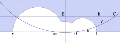
Figure 7. The image of Fig. 6 after a conformal transformation sending $\xi\mapsto\infty$, $0\mapsto 1$ , and $\infty\mapsto-1$. The point $C$ is a point of intersection of $h$ and $\ell$, and $B$ is the intersection of $h$ with the $y$-axis.

Lines and circles are mapped to lines and circles, and angles of incidence are preserved. The horocycle tangent to $\xi$ is now the horizontal line, $h$ (tangent to $\xi$, which has been mapped to infinity). Similarly, the line $\ell$ from zero to infinity passing through the horocycle is now a circle passing through the same points, having the same angle of incidence, $\theta$, with the real line.

We reconstruct this configuration yet again in Fig. 8. Let $A$ be the center of the circle $\ell$, having radius $R=R(\theta)$, let $B$ be the intersection of the horocycle $h$ with the $y$-axis, $C$ the intersection of the horocycle with the circle, and let $D$ denote the origin.

It is easy to see through elementary geometry (since $\overline{A0}$ is tangent to the circle) that angle $0AD=\theta$. Looking at triangle $0AD$, we see that

$$R\sin\theta=\overline{0D}=1.$$ (A.15)

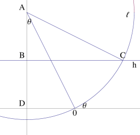
Figure 8. A cleaner version of Fig. 7. The point $A$ is the center of the circle $\ell$, and $D$ denotes the origin.

Let $x=x(\theta)$ represent the length of $\overline{BC}$, and $y=y(\theta)$ be the distance from $B$ to $D$. We aim to compute the precise dependence of $x$ and $y$ on $\theta$.

We collect two identities for $\overline{AB}$:

$$\overline{AB} = \overline{AD}-\overline{BD}=R\cos\theta-y,\text{ and}$$

$$\overline{AB}^{2} = \overline{AC}^{2}-\overline{BC}^{2}=R^{2}-x^{2}.$$

This implies

$$x^{2}=R^{2}-(R\cos\theta-y)^{2}=R^{2}\sin^{2}\theta+2Ry\cos\theta-y^{2},$$

which together with (A.15) gives

$${x^{2}+y^{2}-1\over 2y}={\cos\theta\over\sin\theta}\asymp{1\over\theta},$$ (A.16)

as $\theta\to 0$.

Thus (A.16), together with Proposition A.11, concludes the proof of Theorem A.1.

References

- [Bea83] Alan F. Beardon. The Geometry of Discrete Groups, volume 91 of Graduate Texts in Mathematics. Springer-Verlag, New York, 1983.
- [BG07] Jean Bourgain and Alex Gamburd. Uniform expansion bounds for Cayley graphs of , 2007. Preprint.
- [BGS06] Jean Bourgain, Alex Gamburd, and Peter Sarnak. Sieving and expanders. C. R. Math. Acad. Sci. Paris, 343(3):155–159, 2006.
- [BGS08] Jean Bourgain, Alex Gamburd, and Peter Sarnak. Affine linear sieve, expanders, and sum-product, 2008.
- [CHH88] M. Cowling, U. Haagerup, and R. Howe. Almost matrix coefficients. J. Reine Angew. Math., 387:97–110, 1988.
- [Dal00] F. Dal’bo. Topologie du feuilletage fortement stable. Ann. Inst. Fourier (Grenoble), 50(3):981–993, 2000.
- [DH97] H. Diamond and H. Halberstam. Some applications of sieves of dimension exceeding 1. In Sieve methods, exponential sums, and their applications in number theory (Cardiff, 1995), volume 237 of London Math. Soc. Lecture Note Ser., pages 101–107. Cambridge Univ. Press, Cambridge, 1997.
- [DHR88] H. Diamond, H. Halberstam, and H.-E. Richert. Combinatorial sieves of dimension exceeding one. J. Number Theory, 28(3):306–346, 1988.
- [Gam02] Alex Gamburd. On the spectral gap for infinite index “congruence” subgroups of . Israel J. Math., 127:157–200, 2002.
- [GR07] I.S. Gradshteyn and I.M. Ryzhik. Table of Integrals, Series, and Products. Academic Press, 2007.
- [GT09] B. Green and T. Tao. Linear equations in primes, 2009. To appear, Annals Math. Preprint at arXiv:math/0606088v2.
- [GV88] Ramesh Gangolli and V. S. Varadarajan. Harmonic analysis of spherical functions on real reductive groups, volume 101 of Ergebnisse der Mathematik und ihrer Grenzgebiete [Results in Mathematics and Related Areas]. Springer-Verlag, Berlin, 1988.
- [HL22] G. H. Hardy and J. E. Littlewood. Some problems of ‘Partitio Numerorum’: III. on the expression of a number as a sum of primes. Acta Math., 44:1–70, 1922.
- [HR74] H. Halberstam and H.-E. Richert. Sieve methods. Academic Press [A subsidiary of Harcourt Brace Jovanovich, Publishers], London-New York, 1974. London Mathematical Society Monographs, No. 4.
- [Iwa78] Henryk Iwaniec. Almost-primes represented by quadratic polynomials. Invent. Math., 47:171–188, 1978.
- [Kna86] Anthony W. Knapp. Representation theory of semisimple groups, volume 36 of Princeton Mathematical Series. Princeton University Press, Princeton, NJ, 1986. An overview based on examples.
- [KO08] A. Kontorovich and H. Oh. Apollonian circle packings and closed horospheres on hyperbolic 3-manifolds, 2008. Preprint, http://arxiv.org/abs/0811.2236.
- [Kon07] A. V. Kontorovich. The Hyperbolic Lattice Point Count in Infinite Volume with Applications to Sieves. Columbia University Thesis, 2007.
- [Kon09] A. V. Kontorovich. The hyperbolic lattice point count in infinite volume with applications to sieves. Duke J. Math., 149(1):1–36, 2009. http://arxiv.org/abs/0712.1391.
- [KS03] H. Kim and P. Sarnak. Refined estimates towards the Ramanujan and Selberg conjectures. J. Mar. Math. Soc., 16:175–181, 2003.
- [Lan53] Edmund Landau. Handbuch der Lehre von der Verteilung der Primzahlen. 2 Bände. Chelsea Publishing Co., New York, 1953. 2d ed, With an appendix by Paul T. Bateman.
- [Lan02] Serge Lang. Algebra, volume 211 of Graduate Texts in Mathematics. Springer-Verlag, New York, third edition, 2002.
- [LP82] P.D. Lax and R.S. Phillips. The asymptotic distribution of lattice points in Euclidean and non-Euclidean space. Journal of Functional Analysis, 46:280–350, 1982.
- [LS07] Jianya Liu and Peter Sarnak. Integral points on quadrics in three variables whose coordinates have few prime factors, 2007. Preprint.
- [Pat75] S. J. Patterson. The Laplacian operator on a Riemann surface. Compositio Math., 31(1):83–107, 1975.
- [Pat76] S.J. Patterson. The limit set of a Fuchsian group. Acta Mathematica, 136:241–273, 1976.
- [Sar81] Peter Sarnak. Asymptotic behavior of periodic orbits of the horocycle flow and Eisenstein series. Comm. Pure Appl. Math., 34(6):719–739, 1981.
- [SS58] A. Schinzel and W. Sierpiński. Sur certaines hypothèses concernant les nombres premiers. Acta Arith. 4 (1958), 185–208; erratum, 5:259, 1958.