Suzaku Monitoring of the Iron K Emission Line in the Type 1 AGN NGC 5548

Abstract

We present 7 sequential weekly observations of NGC 5548 conducted in 2007 with the Suzaku X-ray Imaging Spectrometer (XIS) in the 0.2-12 keV band and Hard X-ray Detector (HXD) in 10-600 keV band. The iron K$\alpha$ line is well detected in all seven observations and K$\beta$ line is also detected in four observations. In this paper, we investigate the origin of the Fe K lines using both the width of the line and the reverberation mapping method.

With the co-added XIS and HXD spectra, we identify Fe K$\alpha$ and K$\beta$ line at 6.396${}_{-0.007}^{+0.009}$ keV and 7.08${}_{-0.05}^{+0.05}$ keV, respectively. The width of line obtained from the co-added spectra is 38${}_{-18}^{+16}$ eV ($\textrm{FWHM}=4200_{-2000}^{+1800}$ km/s) which corresponds to a radius of 20${}_{-10}^{+50}$ light days, for the virial production of $1.220\times 10^{7}$ M_⊙ in NCG 5548.

To quantitatively investigate the origin of the narrow Fe line by the reverberation mapping method, we compare the observed light curves of Fe K$\alpha$ line with the predicted ones, which are obtained by convolving the continuum light curve with the transfer functions in a thin shell and an inclined disk. The best-fit result is given by the disk case with $i=30^{\circ}$ which is better than a fit to a constant flux of the Fe K line at the 92.7% level (F-test). However, the results with other geometries are also acceptable (P$>$50%). We find that the emitting radius obtained from the light curve is 25-37 light days, which is consistent with the radius derived from the Fe K line width. Combining the results of the line width and variation, the most likely site for the origin of the narrow iron lines is 20-40 light days away from the central engine, though other possibilities are not completely ruled out. This radius is larger than the H$\beta$ emitting parts of the broad line region at 6-10 light days (obtained by the simultaneous optical observation), and smaller than the inner radius of the hot dust in NGC 5548 (at about 50 light days).

1 Introduction

The neutral, photoionized iron K emission line commonly found in the X-ray spectra of active galactic nuclei (AGNs) can be decomposed into a narrow core around 6.4 keV and a broad redshifted component, though sometimes only one of them is present (Fabian et al. 2000; Yaqoob et al. 2001; Nandra et al. 1997, 2007). The broad, relativistic component could be modelled as being emitted from the vicinity of the central black hole and used to determine the parameters of the black hole (e.g. Brenneman & Reynolds 2006). An alternative explanation of this feature is the complex absorption origin (Miller, Turner & Reeves 2008). However, the origin of the narrow component is still unclear, but could be critical to understanding the central structure of AGNs. The narrow width (FWHM $\sim$ several thousand km/s or less, e.g. Yaqoob & Padmanabhan 2004) suggests an origin well outside the continuum producing region. One of the proposed sites is the putative ‘obscuring torus’ (e.g. Nandra 2006) at $\sim$0.1-1 pc. The evaporation radius of the dust can be estimated by $r=1.3L^{1/2}_{\textmd{uv},46}T^{-2.8}_{1500}$ pc (Barvainis 1987), where $L_{\textmd{uv},46}$ is the ultraviolet luminosity in units of 10⁴⁶ ergs/s, and $T_{1500}$ is the evaporation temperature in units of 1500 K. For NGC 5548, since $L_{\textmd{uv},46}\sim 0.01$ and assuming $T_{1500}=1$, the evaporation radius is about 0.1 pc. However, the broad emission lines have similar line widths, so the more compact broad line region (BLR) is another possible location which cannot be ruled out simply. A BLR origin is supported by the quasi-simultaneous optical spectroscopic observation with Chandra observation of NGC 7213 (Bianchi et al. 2008), which shows consistent Fe K and H$\beta$ line widths, and by the rapid $N_{H}$ changes seen in several AGNs (Elvis et al. 2004; Puccetti et al. 2007; Risaliti et al. 2002), which require a BLR-like radius for the $N_{H}\gtrsim 10^{23}$ cm^-2 absorbers. Seen from another angle, these absorbers must re-emit in Fe K.

The lag between the variation of the flux of the continuum and the line can be used to measure the location of an emission line region (Blandford & McKee 1982) and this ‘reverberation mapping’ methodology has been applied to the optical and UV broad emission lines (BELs) with great success (Peterson et al. 2004). However, until now the 10% or greater error on the flux of the 6.4 keV Fe K line (compared with the usual 1%-5% error on the flux of BELs), and the low sampling frequency of the X-ray observations, have made it hard to apply this method to determine lags for Fe K lines, especially on relatively short timescale expected ($\sim$10 days for a BLR origin). For example, Chiang et al. (2000) found the flux of the iron K line in NGC 5548 was consistent with being constant using the four simultaneous observations of ASCA and RXTE within 25 days and another observation after about half a year. However, some response of the Fe K line to the continuum changes has been found. Markowitz et al. (2003) tried this method, analyzing the long-term RXTE spectra for seven sources. Although they found no evidence for correlated variability between the line and continuum, comparable systematic long-term ($\sim$3-4 years) decreases in the line and continuum were present in NGC 5548.

We report here on a series of seven sequential X-ray observations of NGC 5548 by Suzaku, spaced roughly weekly. This observing campaign was designed, among other goals, to constrain the flux of the iron line to about 10% in each observation. This allows us, for the first time, to apply the reverberation mapping technique to Fe K to try to distinguish different geometries of the Fe K emitting region. NGC 5548 is the source best studied by the optical reverberation mapping technique (e.g. Peterson & Wandel 1999) and so has the best determined radial structure. Therefore, it is easy to determine the relative location of the Fe K line emitting region. In previous observations, only the Fe K$\alpha$ line was detected. As we will present in this paper, the K$\beta$ line is also well detected in the Suzaku observations. Although very weak in some observations, K$\beta$ is useful to constrain the ionization state of iron.

The iron line in NGG 5548 has been observed by several X-ray satellites: ASCA spectra suggested a relativistic broad iron K$\alpha$ line in NGC 5548 with $\sigma=340_{-120}^{+190}$ eV (68% error for 4 interesting parameters, Nandra et al. 1997) and $\sigma\sim 400$ eV (Chiang et al. 2000). However, less than two years later, only the narrow K$\alpha$ line was detected in a Chandra observation with much higher energy resolution (38 eV vs 160 eV) but lower S/N (Yaqoob et al. 2001). An XMM-Newton EPIC CCD observation confirmed the Chandra result (Pounds et al. 2003).

In §2, we describe the observations and the procedure of the data reduction. In this paper we intend to investigate the origin of the Fe K line using the reverberation mapping method and the width of the line. Therefore, in §3, we first fit the spectra of each observation to determine the flux of the continuum and the iron line. We then fit the co-added spectra in §3.2 to determine the mean parameters, especially the width of the iron line. In §4.2 and §4.3, we calculate the transfer functions in different geometries and investigate the possible emitting region of iron line. In §5.1, we discuss the possible origin of the iron line. In §5.3, we briefly discuss the implications of the intensity and the equivalent width of iron line. In §6 we give our conclusions. Throughout this paper we adopt the redshift of NGC 5548 obtained from 21 cm H I measurements, i.e. z=0.017175 (de Vaucouleurs et al. 1991). The errors quoted in this paper correspond to 90% confidence level ($\Delta\chi^{2}=2.706$, Avni 1976) if not otherwise specified.

2 Observations and data reduction

2.1 Observations

During 2007 June to 2007 August, NGC 5548 was observed by the CCD X-ray Imaging Spectrometers (XIS 0, 1, and 3) in 0.2-12 keV band (Koyama et al. 2007) and by the Hard X-ray Detector (HXD) in 10-600 keV band (Takahashi et al. 2007) on Suzaku (Mitsuda et al. 2007) seven times for 28.9 ks-38.7 ks each. We denote these as observations 1-7. The details of the observations are summarized in Table 1.

2.2 Data reduction

Following the standard procedures outlined in the “Suzaku Data Reduction (ABC) Guide (version 2)”, we used the updated Charge Transfer Inefficiency (CTI) calibration (Suzaku XIS CALDB 20081110) and screened the events using the xispi (Ftools 6.5) and xselect scripts provided by Suzaku team (we adopted the standard criterion in xis_event.sel and xis_mkf.sel), respectively.

X-ray spectra were extracted using xselect from all the XISs with a circular extraction region of radius 260 arcsec centered on NGC 5548 ($\alpha=$14h 17m 59.5s, $\delta=$+25d 08m 12.4s, J2000). Background spectra were obtained from a larger annulus around the source (but avoiding the calibration sources on the corners of the chips). Response matrices (rmf) and effective area (arf) files were generated with the xisrmfgen and xissimarfgen (estepfile=dense and num_photon=300000), respectively. We then combined the spectra, background, rmf, and arf files from the two front-side illuminated CCDs, XIS 0 and 3, for each observation with addascaspec (we denote the combined spectra by ‘XIS03’). The spectra of XIS 1 are considered separately, as this detector uses a back-side illuminated CCDs.

NGC 5548 was detected by the silicon diode PIN instrument of the HXD, but below the sensitivity limit of the GSO crystal scintillator instrument. We downloaded the tuned non-X-ray background (NXB, version 2.0) files from the Suzaku Guest Observer Facility (GOF) and then merged the good-time interval (GTI) of the NXB with that of the screened event files to produce a common GTI using mgtime. Then the spectra of the source and the NXB were extracted by xselect using the common GTI. And the dead time of the source spectra was corrected by hxddtcor. Since the event rate in the PIN background event file is 10 times higher than the real background to suppress the Poisson errors, the exposure time of the spectra of NXB was increased by a factor of 10. The cosmic X-ray background (CXB) was not taken into account in the NXB file, therefore we also added a CXB component in the spectral fitting using the model given by the ABC guide (Section 7.3.3). The response file ae_hxd_pinxinome3_20080129.rsp was used for observation 1-5, while the response file ae_hxd_pinxinome4_20080129.rsp was used for observation 6 and 7 due to the changes in instrumental settings of Suzaku during different observation epochs. The PIN spectra were multiplied by a constant cross-normalization factor of 1.16 to account for the differences in calibration between XIS and PIN.

3 Spectral fitting

To perform the reverberation mapping calculation, we should first determine the flux of the continuum and the Fe K line. In order to avoid the influence of the complex absorption below 3 keV (Detmers et al. 2008; Steenbrugge et al. 2003), we only analyze the XIS spectra in 3-10 keV band. The warm absorber seen in the $<$3 keV spectra is presented by Krongold et al. (2009). In this paper, we will focus on the property and origin of the iron emission line. A global fit to the entire Suzaku spectral band for the entire campaign will be presented in a subsequent paper.

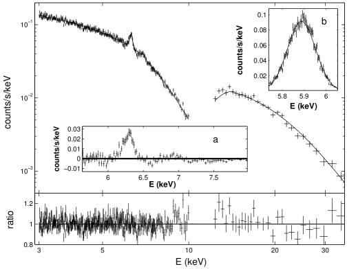
Figure 1: The best fit model (solid lines) and the added spectra of XIS03 (plus). The inset (a) is the residual of the spectra of XIS03 to the best fit of a single power law. The inset (b) is the added spectra of Mn K$\alpha$ line of the calibration sources on XIS03.

For each observation, we fitted the spectra of XIS03 simultaneously with the spectra of XIS 1 in XSPEC (version 12.4). Although both of the energy resolution and the effective area of XIS 1 are lower than XIS 0, 3 in 4-10 keV band (the background level of XIS 1 is also higher than XIS 0, 3 in this band), it is still useful to reduce the error of the intensity of the Fe K line. We fixed the Galactic absorption column at 1.63$\times 10^{20}$ cm^-2 (Murphy et al. 1996), and fitted the spectra with a single power law. The continua were well described by a single power law except for the region of the iron K$\alpha$ and K$\beta$ lines around 6.4 keV and 7.0 keV, respectively (see Figure 1). Therefore, we added two Gaussian lines to describe these features. It is important to construct a self-consistent model to describe all the components of the continuum and theoretically predict the strength of the Fe K line, as in Murphy & Yaqoob (2009). However, this is not the purpose of this paper. Our purpose is only to simply model the Fe K line using a Gaussian line and determine the flux and width of it and then to perform the reverberation calculation. A K$\alpha$ line is required by all the seven spectra ($>$6 $\sigma$), while K$\beta$ line is only required by four observations ($>$2 $\sigma$ for 1, 2, 4, and 7). The 90% upper limit of the flux of the K$\beta$ line is determined in observation 3, 5, and 6. Since the K$\beta$ line is weak, we fixed the width of K$\beta$ to be the same as that of K$\alpha$. Fe K$\beta$ line was also detected in other sources, e.g. NGC 2992 (Yaqoob et al. 2007) and Mrk 3 (Awaki et al. 2008). The detailed result of the fitting is given in Table 3, though we are mainly concerned about the flux of the continuum and the intensity of the Fe K line. Due to the weak reflection component in NCG 5548 (e.g. Pounds et al. 2003), if we simultaneously fit the continua in the XIS and PIN spectra of each observation using the pexrav model instead of the power law model, the intensity of the Fe K line will systematically decrease by 10% for each observation (the strength of the reflection component $R\sim 0.2-1.5$). However, this change will not influence the reverberation mapping result in §4.3, since it degenerates with the normalization of the transfer function (see the detail of the transfer function in §4.2). The PIN data is also not helpful to reduce the error of the flux of the Fe K line due to the additional uncertainty introduced by the reflection component and large error in the PIN spectra. The detailed discussion about the variation of the X-ray continuum and simultaneous UV/optical data will be presented in another paper.

3.1 Continuum light curve

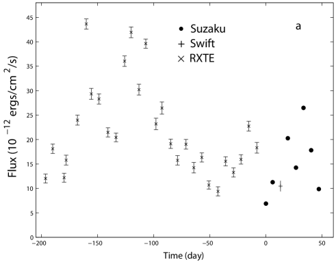
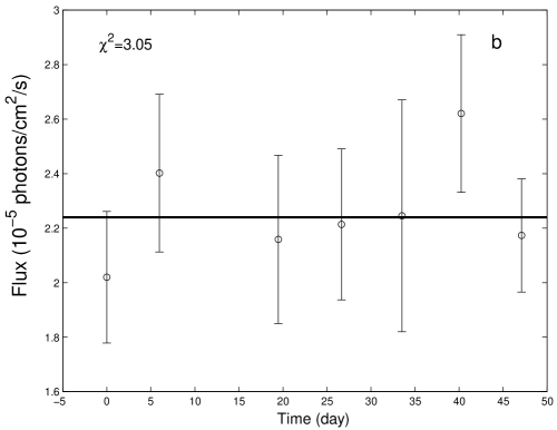
Figure 3: (a) The light curve of the flux of the continuum in 3-10 keV band. The small error bar of the flux of the Suzaku observation is omitted. (b) The light curve of the flux of K$\alpha$ line. The solid line in (b) is the result of the constant fitting (see the text in §4.1).

Having fitted the spectra, we calculated the observed flux of the continuum in the 3-10 keV band. The result light curve is shown in Figure 3a. To better sample the continuum light curve, we also utilized one observation of the continuum from the simultaneous Swift campaign. Since the observation times and the flux of other Swift data are quite similar to that of the Suzaku data, we will not include them in this paper. The details of the Swift campaign will be discussed in Grupe et al. (2009). 28 observations of the continuum with PCA on RXTE before the Suzaku campaign are also used, since we are looking for the lag between the variation of continuum and line. However, due to the short exposure time, we cannot determine the flux of the line in any of these additional observations. The details of the RXTE and Swift observations are summarized in Table 2.

3.2 Narrow iron lines

To determine the mean parameters of the Fe K$\alpha$ and K$\beta$ lines more accurately, especially the width of the line, we added the spectra from the seven observations together using addascaspec (the XIS03, XIS1, and PIN spectra were added separately and then fitted simultaneously). The net counts of the source in 3-10 keV band in the total XIS03 and XIS1 spectra are 160349 and 75332, respectively. The net counts of the source in 12-35 keV band in the total PIN spectra is 22243. We found that the XIS1 spectra could not provide any useful constraint on the width of the Fe K line, since the $\sigma$ of the Gaussian line is pegged at 0 eV (the 90% upper limit is 30 eV). Therefore, we will only utilize the co-added XIS 03 and PIN spectra to determine the width of the Fe K line.

If we only fitted the co-add XIS03 spectra using the model in §3, i.e. a power law and two Gaussian lines, the width is $\sigma=50_{-15}^{+14}$ eV. However, since the weak reflection component could influence the width of the Fe K line, we then simultaneously fitted the co-added XIS 03 and PIN spectra using the pexrav model and two Gaussian lines. The derived parameters are given in Table 4, where the strength of the reflection component ($R\sim 0.8$) could explain the Fe K line. As shown in Figure 1, only a narrow iron line is clearly present in the spectra, with a width, $\sigma=$38${}_{-18}^{+16}$ eV. This value is consistent with previous results: i.e. $\sigma=$41${}_{-24}^{+32}$ eV obtained by HEG+MEG on Chandra (Yaqoob et al. 2001) and $\sigma=$40${}_{-40}^{+40}$ eV (MOS) and 64${}_{-24}^{+24}$ eV (PN) obtained by XMM-Newton (Pounds et al. 2003).

Since the peak energies of the line and the parameters of the continua are somewhat different for each observation, we simultaneously fitted the spectra of all observations in XSPEC to test whether the line was broadened artificially in the co-added process. We required the width of line to be the same for all observations and kept other parameters free. The obtained width is only slightly smaller than that from the co-add spectra by about 2 eV, which implies the co-added method has not significantly broadened the width.

The width obtained by the co-add spectra is inconsistent with zero at 2.2 $\sigma$ and corresponds to FWHM= 4200 km/s and a radius of 5.2$\times 10^{16}$ cm or 5.2$\times 10^{3}$ $r_{g}$ ($r_{g}=GM/c^{2}$), for the 6.71$\times$10${}^{7}M_{\odot}$ black hole in NGC 5548 (Peterson et al. 2004). In §5.1, we will estimate the location of the emitting material of the line and discuss the origin of the line.

To test the presence of the broad, relativistic Fe K$\alpha$ line found by ASCA, we tried the diskline model in XSPEC to fit the K$\alpha$ line. We fixed the inner and outer disk radii at 6$r_{g}$ and 1000$r_{g}$ ($r_{g}=GM/c^{2}$), respectively. The index of the power law emissivity was frozen at -2.5 (the mean value obtained in Nandra et al. 1997). If we thaw the index, it will be pegged at the positive upper limit in XSPEC, i.e., the flux of the line is dominated by the outer disk and therefore it is not a disk line at all. It was found that the diskline model cannot describe the K$\alpha$ line alone, since $\chi^{2}$ was higher by 128 than for a narrow line with the same number of parameters. The same conclusion was also obtained by Yaqoob et al. (2001).

Next, we investigated the result if we fit the K$\alpha$ line with a disk line and a Gaussian line. Besides the constraint on the diskline model mentioned above, we also fixed the value of the inclination angle at 31 degrees, which is the best-constrained value from the ASCA data (Yaqoob et al. 2001). We found the central value of the intensity of the disk line is pegged at 0 and the 90% upper limit is $4\times 10^{-6}$ photons/cm²/s. Therefore, any broad component must be $>$ 5 times weaker than the narrow component and we will not include this component in the following discussion.

We show the confidence regions for the peak energies of K$\alpha$ and K$\beta$ in Figure 2a. The expected values of different iron ionization states (Palmeri et al. 2003; Mendoza et al. 2004; Yaqoob et al. 2007) are also shown. Since the peak energy may be influenced by the residuals in the energy scale calibration, we extracted the spectra of the ⁵⁵Fe calibration sources on the corners of the CCDs and added them together (see the inset in Figure 1b). Using a Gaussian line to fit the Mn K$\alpha$ line, we found the peak energies are 5.892${}_{-0.001}^{+0.001}$ keV and 5.893${}_{-0.001}^{+0.002}$ keV for XIS03 and XIS1, respectively. The expected value of the Mn K$\alpha$ line is 5.895 keV. This result is well within the accuracy of the absolute XIS energy scale given by the Suzaku Technical Description as 0.2%. The fit widths of Mn K$\alpha$ line are 12${}_{-5}^{+3}$ eV and 16${}_{-8}^{+5}$ eV for XIS03 and XIS1, respectively. Therefore, the peak energy obtained by the spectral fitting is reliable and we could conclude that the iron emission line in NGC 5548 is most likely to be dominated by relatively low ionization states, $<$Fe XIII (99% confidence). Actually, the observed Fe K line could be a blend of several ionization states.

The confidence regions of the intensities of the Fe K$\alpha$ and K$\beta$ lines are shown in Figure 2b. The expected ratio of I(K$\beta$) to I(K$\alpha$) varies from 0.12 to 0.20 for different ionization states (dashed lines in Figure 2b, Palmeri et al. 2003; Mendoza et al. 2004;). Our result is fully consistent with the expected value. However, due to the weakness of K$\beta$, the error is still too large to constrain the ionization state precisely.

4 Time variability analysis

4.1 Fe K$\alpha$ line light curves

The light curve of Fe K$\alpha$ line is shown in Figure 3b each being determined to $\sim$10%. As K$\beta$ is weak in some observations, we will only discuss the result for K$\alpha$ below. As shown in Figure 3a, the flux of the continuum changed strongly during the seven observations. The highest value (2.65$\times 10^{-11}$ ergs/cm²/s, for observation 5) is about 4 times that of the lowest (6.89$\times 10^{-12}$ ergs/cm²/s, for observation 1). However, perhaps due to the relatively large error, the flux of the line is consistent with being constant, $\chi_{min}^{2}=$3.05 (P=80%) and the value of the corresponding line constant flux is 2.24$\times 10^{-5}$ photons/cm²/s.

A constant Fe K$\alpha$ flux is the simplest solution to the Fe K$\alpha$ light curve, and it requires the emitting region should be far from the central engine to smooth out the variation in short time scale. According to the result in §4.3 and Figure 6b, it should be larger than 100 light days. However, as shown in Figure 1 and 2 in Markowitz et al. (2003), the presence of the variation of the Fe K flux in time scale shorter than 100 days indicates the emitting region must be smaller than 100 light days. The emitting region required by the constant flux fitting is also inconsistent with that required by the line width (see §5.1). Therefore, we have investigated whether there is a better and more self-consistent solution than the constant flux fitting. To quantitatively access the emitting location of the Fe K$\alpha$ line, we should perform the reverberation calculation. The cross-correlation function (CCF) is usually used in the optical reverberation mapping to determine the lag between the continuum and the emission line. However, due to the very few data points of the light curve of the Fe K line and the large error of them, we did not find any significant peak in CCF. Therefore, we will approach this problem in a different way. To do so we first calculate the transfer function for Fe K$\alpha$ in §4.2.

4.2 Transfer function

As in the case of the optical broad emission lines, we calculate a transfer function for Fe K$\alpha$, i.e. the response of the flux of the line to a $\delta$ function change in the continuum. We consider two cases: (1) a spherical region and (2) an inclined disk.

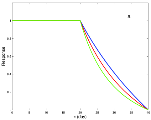
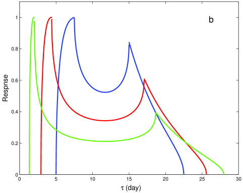
Figure 4: The transfer functions for the spherical (a) and disk cases (b). We choose $r_{min}=10$ light days and $r_{max}=20$ light days for all curves, which are normalized to 1 at the maximum. (a) $\alpha=2$ (blue), $\alpha=3$ (red), and $\alpha=4$ (green). (b) $\alpha=3$ for all curves. $i=30^{\circ}$ (blue), $i=45^{\circ}$ (red), and $i=60^{\circ}$ (green).

(1) We assume the emitting material is spherically distributed around the center with an inner ($r_{min}$) and outer ($r_{max}$) radius. The transfer function in this model is then simply a constant between 0 and $2r_{min}/c$, and then decays to 0 at $2r_{max}/c$ (see Figure 4a and Peterson 1993).

(2) For a thin disk, the general form of the transfer function is two-peaked (Welsh & Horne 1991). Figure 4b shows the result for different values of the inclination angle $i$ (the angle between the normal of the disk and the line of sight).

The shape of the transfer function depends on the form of the “responsivity” $\varepsilon(r)$ (see Figure 4a), which combines the effects of the distributions of the number density of clouds and the emissivity per cloud. We assumed that the responsivity is a power law $\varepsilon(r)\varpropto r^{-\alpha}$ and the normalization is adjusted to fit the observed light curve. The power law form is simple and somewhat arbitrary. However, since we only consider the thin shell case (i.e. $\Delta r\ll r$, or equivalent to the locally optimized clouds model), the result is not sensitive to the detailed form of the responsivity nor the index of the power law (see Figure 6a). $\alpha=3$ is adopted in the calculation in §4.3.

We could then obtain the predicted light curve of the line by convolving the transfer function with the light curve of the continuum flux. In the thin spherical shell and disk cases discussed in §4.3, it can be proved that the the lag time, $\tau$, obtained by the CCF just corresponds to the radius of the emitting region, i.e. $\tau=r/c$ (Koratkar & Gaskell 1991).

4.3 Comparison with the observed light curve

Since the observation data of the continuum are still too few to produce a complete light curve, we performed linear interpolation between data points to convolve the light curve with the transfer function.

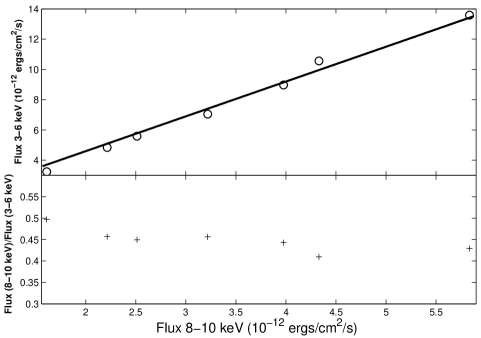
Figure 5: The top panel shows the correlation between the flux in 3-6 keV band and that in 8-10 keV band of all seven observations. The solid line is the best-fitting straight line across the origin. The error bars of the fluxes are omitted, since they are smaller than the symbols. The bottom panel shows the ratios between the flux in 8-10 keV band and that in 3-6 keV band.

We used the light curve of the continuum in 3-10 keV band in order to have precision measurements. Similar bands (e.g. 2-10 keV) have been adopted in the previous attempts to determine the lag between the variation of the continuum and the Fe K line (e.g. Markowitz et al. 2003, 2009), although only photons from above the ionization threshold can actually lead the emission of an Fe K photon. As shown in Figure 5, the flux in 3-6 keV band is tightly and nearly proportionally correlated with the flux in 8-10 keV band. Any possible effects due to rapidly changing $N_{H}$ (Risaliti et al. 2005) must therefore be small. As a result, the results of the following calculations will not be sensitive to the adopted energy band of the continuum. The change of the continuum slope is also related to the total amount of the ionization flux. However, this is a minor factor compared with the change of the normalization of the continuum. Specially, this effect should be even small for NGC 5548, since e.g. Sobolewska and Papadakis (2009) showed that the continuum slope is nearly independent on the flux. We find the same lack of dependence (Table 3).

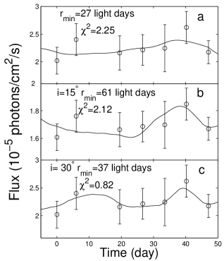
Figure 7: The comparison between the observed and predicted light curve of the flux of the line with the minimum of $\chi^{2}$ in different cases, i.e. (a) spherical case, (b) disk case with $i=15^{\circ}$, (c) disk case with $i=30^{\circ}$.

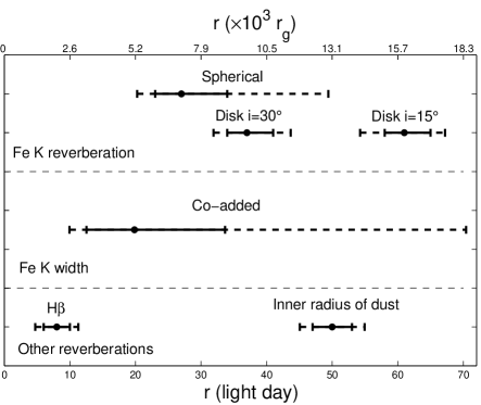
Figure 9: The summary of the location of the Fe K$\alpha$ line emitting region. We show intervals derived from the variation of the flux and the width of the Fe K line, with the locations of H$\beta$ and the inner radius of the dust for comparison. The solid and dashed error bars correspond to 68% and 90% confidence intervals, respectively.

We fixed the width of the emitting region at 0.1 light days, substantially smaller than the likely radius of the Fe K emitting region, and varied $r_{min}$. After convolving the light curve of the continuum with the transfer functions in different geometries and $r_{min}$, we compared the predicted light curve of the line with the observed one to find the minimum value of $\chi^{2}$ (since the error on the flux is asymmetric, we conservatively adopt the larger one to calculate $\chi^{2}$). Figure 6b shows $\chi^{2}$ vs $r_{min}$. All the curves show pronounced minima (somewhat surprisingly, given the weak structure in the Fe K$\alpha$ light curve) and finally decrease towards the result of the constant fitting (the horizontal dashed in Figure 6b) with increasing $r_{min}$, as the result of the significant smoothing effect with large $r_{min}$. The values of minimum $\chi^{2}$ in the spherical thin shell case and disk case with $i=15^{\circ}$ and $i=30^{\circ}$ are well below that of the constant fitting, and we will only discuss these three cases below. With the smallest value of $\chi^{2}$, the best-fitting light curve in the disk with $i=30^{\circ}$ is improved at 92.7% level compared with the constant fitting. We show the predicted light curves corresponding to the minima of $\chi^{2}$ in these three cases in Figure 7. Due to the few data points, we cannot tightly constrain the inclination angle. Except for the the disk case with $i=15^{\circ}$, the positions of the minimum $\chi^{2}$ in the spherical case (27 ${}_{-7}^{+22}$ light days) and the disk case with $i=30^{\circ}$ (37 ${}_{-5}^{+7}$ light days) are similar, and they are smaller than the inner radius of the dust (47-53 light days, see the discussion in §5.1). The value of the best-fitting $r_{min}$ in the disk case with $i=15^{\circ}$ is 61${}_{-7}^{+6}$ light days, which is beyond the inner radius of the dust of NGC 5548 (such optically thick region will significantly absorb the photons of Fe K lines) and only marginally consistent with the small tail of the 90% confidence interval of the emitting region inferred from the widths of Fe K$\alpha$ line (see the error bar in Figure 9 and it should be noted that the error bar is quite asymmetric). In addition, $i=15^{\circ}$ is also well smaller than the best-fitting inclination angle of the disk line in the ASCA ($i=31.5^{\circ}\pm 6.5^{\circ}$, Yaqoob et al. 2001), though it is not very reliable, due to the absence of the broad component of the Fe K line in the following Chandra, XMM-Newton, and our Suzaku observations. Therefore, the disk case with $i=15^{\circ}$ is quite unlikely, and we will only focus on the spherical case and the disk case with $i=30^{\circ}$ when discussing the origin of the narrow Fe K$\alpha$ line in detail in §5.1.

5 Discussion

5.1 Location of the Fe K emitting region

Assuming the geometry and dynamics of the emitting region of the Fe K line are the same as that of the H$\beta$ line, and using the virial relation for the H$\beta$ line, $\sigma^{2}r/G=1.220\times 10^{7}$ M_⊙ (Peterson et al. 2004), the radius of the Fe K emitting region can be derived using the Fe K$\alpha$ width, $\sigma$, obtained in §3.2. The derived radius using the width obtained by the co-added XIS03 and PIN spectra is 20${}_{-10}^{+50}$ light days.

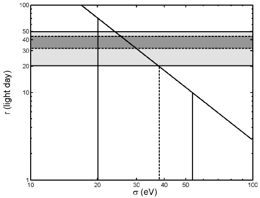
Figure 8: The relationship between $\sigma$ of the line and the radius of the emitting region inferred from the black hole mass. The vertical dashed and solid lines correspond the central value and the 90% confidence intervals of the line width obtained by the co-added XIS 03 and PIN spectra, respectively. The horizontal lines correspond to the 90% confidence intervals of the emitting region inferred from the light curve in the spherical case (solid) and the disk case with $i=30^{\circ}$ (dashed, see Figure 6c).

In Figure 8, we plot the line width size against $r_{min}$ from the reverberation analysis (Figure 6b) for both the spherical thin shell case and the disk case with $i=30^{\circ}$ with 90% confidence intervals for both quantities. The disk case with $i=30^{\circ}$ and the spherical case are consistent with the width of the co-added Fe K$\alpha$ line . Combining the above results, we conclude that the origin of the narrow iron line in NGC 5548 is likely to be $\sim 20-40$ light days away from the continuum source, for the geometries considered. However, the other possible origins are not completely ruled out due to the incompleteness of the light curves, our model-dependent method, and the sizeable error on the width of the Fe K line.

Since NCG 5548 is one of the best-studied AGNs with reverberation mapping, the locations of the BELs are well-determined, especially for the H$\beta$ line. The lag between the flux of H$\beta$ line and the continuum varies from 6.5 light days to 26.5 light day depending on the luminosity of the continuum (Bentz et al. 2007; Cackett & Horne 2006). Since the correlation between the lag time and the continuum flux is more significant than the correlation between the lag time and the width of H$\beta$ line (Bentz et al. 2007), and the broad component of the H$\beta$ line is weak during the Suzaku campaign, we will utilize the continuum flux to predict the radius of the H$\beta$ line region.

From the simultaneous optical spectra of NGC 5548 from FLWO FAST spectrograph (June 19-23, 2007), we measured the monochromatic flux at 5100 Å and used this flux to estimate the radius of the H$\beta$ emitting region at the time of the Suzaku campaign. After calibration with a standard star, the optical spectra were put on an absolute calibration scale assuming a constant flux of $F$([OIII] 5007)${}_{\textrm{standard}}$ = 5.58$\times$10^-13 ergs/s/cm² (Peterson et al. 1991) and found the monochromatic flux at 5100 Å, $F(5100{\textmd{ \AA}})_{\textmd{observed}}$ = 5.13$\times$10^-15 ergs/s/cm${}^{2}/$Å. For the aperture size of $5\textmd{ arcsec}\times 7.5\textmd{ arcsec}$, the contribution of the host galaxy at 5100 Å is 4.47$\times$10^-15 ergs/s/cm${}^{2}/$Å (Bentz et al. 2006). To account for the effect of the aperture and the difference between telescopes, the flux measured by FLWO should be converted by the coefficients given in Peterson et al. (2002), i.e. $F(5100{\textmd{ \AA}})_{\textmd{true}}=\varphi F(5100{\textmd{ \AA}})_{\textmd{observed}}-G$. We averaged the results using the different coefficients (i.e. $\varphi$ and $G$) determined in years 8 and 9-13 of the campaign (see details in Peterson et al. 2002), and then excluded the flux of the host galaxy (4.47$\times$10^-15 ergs/s/cm${}^{2}/$Å, Bentz et al. [2006]) . The final 5100 Å flux of the AGN in NGC 5548 is $(1.7\pm 0.7)\times 10^{-15}$ ergs/s/cm${}^{2}/$Å during the Suzaku campaign. With the relation between the emitting region of H$\beta$ line and $F$(5100 Å) (Figure 5 in Bentz et al. [2007]), we found r(H$\beta$)= $8\pm 2$ light days during the Suzaku observations.

From the result of dust reverberation of NGC 5548, we also know the inner radius of the hot dust in this source is 47-53 light days (from the lag of K-band relative to V-band, Suganuma et al. 2006).

We plot the radial locations of Fe K$\alpha$, H$\beta$ and the inner dust in Figure 9 (note that this is a linear plot). It is likely that the location of the Fe K emitting region is closer in than the inner radius of the dust, but slightly farther out than H$\beta$, i.e. the origin of the narrow iron line lies in the outer part of the BLR [$(0.5-1.0)\times 10^{4}$ $r_{g}$]. This result is consistent with the region emitting the optical Fe II emission lines, which is less than several light weeks from the continuum emitter (Vestergaard & Peterson 2005). This region is also consistent with the intermediate line region proposed by Zhu et al. (2009) and the radius of the low ionization, low velocity component of the warm absorber in NGC 5548 (r$<$3 pc, Krongold et al. 2009). Despite the uncertainty of the column density of the Fe K emitting region, it is surely much higher (see §5.3) than that of the warm absorber found in NGC 5548 ($10^{21}\sim 10^{22}$ cm^-2, Krongold et al. 2009). Therefore, It clearly does not lie along our line of sight.

5.2 Physical condition

We can use the location derived above to estimate the density of the emitting region from the ionization parameter and the distance. Kallman et al. (2004) investigated the dependence of the line profile of K$\alpha$ and K$\beta$ on the ionization parameter. The peak energies of K$\alpha$ and K$\beta$ in NGC 5548 (see Figure 2a) prefer a relatively low ionization parameter, i.e. $\log\xi=-1\pm 1$, where $\xi=L/nR^{2}$ $(\textmd{erg s${}^{-1}$cm})$, $L$ is the Fe K ionizing luminosity of the continuum source (erg s^-1), $n$ is the density of the emitting region (cm^-3), and $R$ is the distance to the continuum source (cm). With $\log L=43.7\pm 0.3$, $\log\xi=-1\pm 1$, and $R=30\pm 10$ light days, we obtain $\log n=10.9\pm 1.1$, which is comparable with the density of the gas in the BLR of NGC 5548 (Ferland et al. 1992; Goad & Koratkar 1998; Kaspi & Netzer 1999).

5.3 Theoretical intensity of the Fe line

The intensity and the equivalent width of the iron line can be estimated theoretically (Krolik & Kallman 1987; Yaqoob et al. 2001). We found the column density $N_{H}>10^{23}$ cm^-2 is required to produce the observed intensity and the equivalent width of the Fe K$\alpha$ line in our Suzaku observations. However, as pointed out by Miller et al. (2009) and Yaqoob et al. (2009), due to the self-absorption effect and the Compton scattering, for $N_{H}>10^{23}$ cm^-2, the relation between the intensity of the Fe K line and $N_{H}$ or the abundance of iron is quite non-linear, and the intensity of the Fe K line also significantly depends on the geometry of the emitting region and the observing angle. Since the detailed investigation of the geometry, $N_{H}$, and the abundance of the emitting region of Fe K lines is much beyond the scope of this paper, we will not further discuss the constraints obtained from the intensity and the equivalent width of the Fe K lines.

6 Conclusions

We analyzed the iron K$\alpha$ and K$\beta$ lines in spectra of NGC 5548 obtained by Suzaku XIS and summarize our results as follows.

1. The iron K$\alpha$ line was well detected ($>6\sigma$) in all seven observations and the K$\beta$ line was also detected ($>2\sigma$) in four observations (1, 2, 4, and 7).

2. Only a narrow iron line was found in the spectra. The line width obtained by the added spectra is 38${}_{-18}^{+16}$ eV, which is consistent with the results of Chandra and XMM-Newton. Assuming the same virial relation as that of the H$\beta$ line, this width corresponds to a radius of 20${}_{-10}^{+50}$ light days. Any relativistically broadened disk line must be a factor of 5 weaker than the narrow component in flux at 90% confidence level.

3. We compared the observed peak energies and intensity ratios of K$\alpha$ and K$\beta$ lines with the expected value and found they are consistent with the low ionization states of iron, i.e. lower than Fe XIII, at the 99% confidence level.

4. The Fe K$\alpha$ line is consistent with being constant over the 50 days of the Suzaku campaign, although the 3-10 keV continuum varies by a factor of 4. It is shown that a location at $>$100 light days is consistent with the data (see the discussion in §4.3 and Figure 6b), but this is not a unique result.

5. To further access the location of the iron lines using the light curve, we calculated the transfer functions in spherical and disk geometries, and compared the predicted light curves with the observed one. The value of $\chi^{2}$ is smallest in the disk case with $i=30^{\circ}$, which is better than the constant fitting at the 92.7% level. The spherical thin shell case is also acceptable (P=81%). The inferred emitting radii are 27${}_{-7}^{+22}$ light days in the spherical case and 37${}_{-5}^{+7}$ light days in the disk case with $i=30^{\circ}$, which are consistent with that obtained from the width of iron lines.

6. Combining the Suzaku constraints, the most likely origin of the narrow iron lines is about 20-40 light days away from the central engine, i.e. the outer part of BLR (5.2$\times 10^{3}$-1.0$\times 10^{4}$ $r_{g}$). However, we could not completely rule out other possible origins.

The approaches used in this paper offer a valuable tool for determining the size and structure of the inner regions of AGNs, although we stress again this method is model dependent. The constraint on the emitting region of the narrow Fe K line obtained by the width will be greatly improved by upcoming calorimeters, which have $>10$ time better the energy resolution, of only a few eV. If future X-ray satellites (e.g. Astro-H, IXO, and Gen-X) with larger effective area could reduce the error of the flux of the Fe K emission line by even a factor of 2, then it will be possible to distinguish different geometries from the constant flux fitting. Higher sampling frequency campaign, preferably over a longer baseline, is also desirable to obtain a cross-correlation function with a quality comparable to or better than current optical observations.

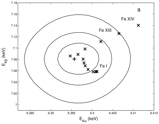
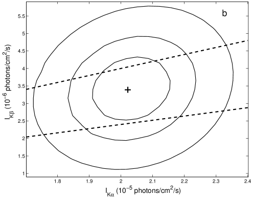
Figure 2: The confidence region of the peak energies (a) and intensities (b) of K${\alpha}$ and K$\beta$ obtained from the fitting of the co-added XIS03 and PIN spectra. The contours from inner to outer correspond to $\Delta\chi^{2}$=1.00, 2.71, and 6.63 (68%, 90%, 99%), respectively. The crosses in (a) are the predicted values of the peak energies in different ionization states of iron. The lower and upper dashed lines in (b) correspond to the I(K$\beta$)/I(K${\alpha})$ ratios of 0.12 and 0.20, respectively.

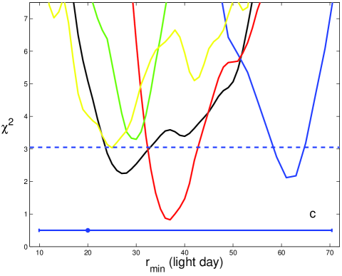
Figure 6: (a) Comparison with different values of $\alpha$ in the spherical case. $\alpha=2$ (blue), $\alpha=3$ (red), and $\alpha=4$ (green). Since the original curves are nearly identical, the curves of $\alpha=2$ and $\alpha=4$ are vertically shifted by -0.5 and 0.5, respectively. (b) The curves of $\chi^{2}$ with different $r_{min}$ for spherical and disk cases. Spherical (black), disk $i=15^{\circ}$ (blue), $i=30^{\circ}$ (red), $i=45^{\circ}$ (green), and $i=60^{\circ}$ (yellow). The horizontal dashed line is the $\chi^{2}$ of the constant fitting (see the text). (c) Enlarged plot of (b). The error bar at the bottom is the 90% confidence interval inferred from the line width obtained by the simultaneous fitting of all spectra (see Figure 8).

Table 1: Suzaku observation log.

Sequence number	Obs. ID	Start Date & Time	Exposure time (ks)	3-10 keV Count Rate
				($10^{-3}$ photons/cm2/s)
1	702042010	2007-06-18 UT 22:28:15	31.1	0.772
2	702042020	2007-06-24 UT 21:53:31	35.9	1.29
3	702042040	2007-07-08 UT 10:02:55	30.7	2.35
4	702042050	2007-07-15 UT 13:57:39	30.0	1.62
5	702042060	2007-07-22 UT 10:40:25	28.9	3.05
6	702042070	2007-07-29 UT 04:20:44	31.8	2.04
7	702042080	2007-08-05 UT 00:37:46	38.8	1.12

Table 2: RXTE and Swift observation logs.

Obs. ID	Start Date & Time	Exposure time (s)	3-10 keV Flux
			($10^{-12}$ ergs/cm2/s)
RXTE
92113-07-40-00	2006-12-05 UT 03:35:48	919	12.0 $\pm$ 0.9
92113-07-41-00	2006-12-11 UT 12:59:06	885	18.1 $\pm$ 1.0
92113-07-42-00	2006-12-21 UT 16:34:27	961	12.2 $\pm$ 0.9
92113-07-43-00	2006-12-23 UT 11:08:04	830	15.8 $\pm$ 1.0
92113-07-44-00	2007-01-02 UT 13:09:22	914	24.0 $\pm$ 1.0
92113-07-45-00	2007-01-10 UT 10:09:27	1259	43.6 $\pm$ 1.0
92113-07-46-00	2007-01-14 UT 21:15:16	926	29.3 $\pm$ 1.1
92113-07-47-00	2007-01-21 UT 16:35:22	913	28.3 $\pm$ 1.0
92113-07-48-00	2007-01-29 UT 17:19:33	948	21.5 $\pm$ 0.9
92113-07-49-00	2007-02-05 UT 20:22:13	1171	20.4 $\pm$ 0.9
92113-07-50-00	2007-02-13 UT 12:12:30	895	36.0 $\pm$ 1.1
92113-07-51-00	2007-02-19 UT 08:05:31	896	41.9 $\pm$ 1.1
92113-07-52-00	2007-02-26 UT 07:25:07	1002	30.2 $\pm$ 1.1
92113-07-53-00	2007-03-04 UT 07:48:42	1354	39.6 $\pm$ 0.9
92113-07-54-00	2007-03-13 UT 11:30:51	614	23.2 $\pm$ 1.2
92113-07-55-00	2007-03-18 UT 18:56:43	572	26.4 $\pm$ 1.3
92113-07-56-00	2007-03-26 UT 13:58:42	994	19.1 $\pm$ 0.9
92113-07-57-00	2007-04-01 UT 16:10:48	982	15.7 $\pm$ 1.0
92113-07-58-00	2007-04-09 UT 04:12:03	893	19.0 $\pm$ 1.0
92113-07-59-00	2007-04-16 UT 03:23:00	955	14.2 $\pm$ 1.1
92113-07-60-00	2007-04-23 UT 06:05:57	961	16.3 $\pm$ 0.9
92113-07-61-00	2007-04-29 UT 12:54:16	1041	10.7 $\pm$ 0.8
92113-07-62-00	2007-05-07 UT 17:14:43	928	9.4 $\pm$ 0.9
92113-07-63-00	2007-05-14 UT 11:42:04	950	15.5 $\pm$ 0.9
92113-07-64-00	2007-05-21 UT 11:48:48	922	13.3 $\pm$ 0.9
92113-07-65-00	2007-05-28 UT 03:30:13	931	15.9 $\pm$ 1.0
92113-07-66-00	2007-06-04 UT 01:59:35	949	22.7 $\pm$ 1.0
92113-07-67-00	2007-06-11 UT 07:33:05	888	18.3 $\pm$ 1.1
Swift
00030022061	2007-07-01 UT20:25:01	2503.18	10.5

Table 3: The derived parameters from the spectral fits of the XIS data of each observation (with error corresponding to 90% confidence level except flux and intensity).

Sequence	Continuum		K$\alpha$				K$\beta$
number	$\Gamma$	Flux	E	$\sigma$	I	EW	E	I	EW	$\chi^{2}$/dof	$\Delta\chi^{2}_{1}\;\tablenotemark{h}$	$\Delta\chi^{2}_{2}\;\tablenotemark{i}$
1	1.41${}_{-0.06}^{+0.07}$	6.89${}_{-0.34}^{+0.24}$	6.405${}_{-0.017}^{+0.016}$	44${}_{-44}^{+32}$	2.02${}_{-0.24}^{+0.23}$	215${}_{-77}^{+83}$	7.00${}_{-0.08}^{+0.08}$	5.6${}_{-1.8}^{+1.7}$	68${}_{-68}^{+72}$	78.9/114	10.2	122.4
2	1.55${}_{-0.05}^{+0.05}$	11.28${}_{-0.30}^{+0.23}$	6.384${}_{-0.016}^{+0.017}$	46${}_{-46}^{+29}$	2.40${}_{-0.29}^{+0.25}$	155${}_{-56}^{+58}$	7.08${}_{-0.06}^{+0.06}$	5.5${}_{-2.0}^{+2.0}$	42${}_{-42}^{+51}$	197.7/177	7.4	122.8
3	1.68${}_{-0.03}^{+0.03}$	20.25${}_{-0.16}^{+0.13}$	6.374${}_{-0.025}^{+0.027}$	62${}_{-37}^{+31}$	2.16${}_{-0.31}^{+0.30}$	77${}_{-38}^{+39}$	7.04	$<$5.5	$<$40	355.1/338		65.7
4	1.53${}_{-0.04}^{+0.04}$	14.24${}_{-0.27}^{+0.24}$	6.380${}_{-0.018}^{+0.019}$	34${}_{-34}^{+31}$	2.21${}_{-0.27}^{+0.28}$	112${}_{-48}^{+48}$	7.05${}_{-0.04}^{+0.04}$	7.5${}_{-2.1}^{+2.2}$	44${}_{-44}^{+44}$	227.3/214	11.7	98.9
5	1.61${}_{-0.03}^{+0.03}$	26.46${}_{-0.16}^{+0.14}$	6.401${}_{-0.031}^{+0.029}$	62${}_{-62}^{+49}$	2.25${}_{-0.36}^{+0.43}$	61${}_{-34}^{+34}$	7.04	$<$5.3	$<$31	427.9/406		54.6
6	1.57${}_{-0.03}^{+0.03}$	17.80${}_{-0.22}^{+0.18}$	6.393${}_{-0.015}^{+0.015}$	34${}_{-34}^{+29}$	2.62${}_{-0.26}^{+0.29}$	106${}_{-39}^{+39}$	7.04	$<$7.0	$<$50	303.2/308		124.1
7	1.53${}_{-0.04}^{+0.04}$	9.85${}_{-0.24}^{+0.20}$	6.416${}_{-0.012}^{+0.012}$	23${}_{-23}^{+28}$	2.17${}_{-0.21}^{+0.19}$	162${}_{-53}^{+52}$	6.97${}_{-0.08}^{+0.09}$	4.0${}_{-1.6}^{+1.5}$	34${}_{-34}^{+43}$	205.0/216	6.9	166.1

Table 4: The derived parameters from the spectral fits of the co-added XIS03 and PIN data (with error corresponding to 90% confidence level except flux and intensity).

Sequence

Continuum

K$\alpha$

K$\beta$

number

$\Gamma$

E${}_{\textrm{cut-off}}$

R

Flux

E

$\sigma$

I

EW

E

I

EW

$\chi^{2}$/dof

$\Delta\chi^{2}_{1}\;$

$\Delta\chi^{2}_{2}\;$

1

1.59${}_{-0.03}^{+0.03}$

75${}_{-15}^{+85}$

0.79 ${}_{-0.32}^{+0.35}$

15.1${}_{-0.3}^{+0.1}$

6.396${}_{-0.007}^{+0.009}$

38${}_{-18}^{+16}$

2.02${}_{-0.11}^{+0.13}$

95${}_{-19}^{+21}$

7.08${}_{-0.05}^{+0.05}$

3.4${}_{-0.9}^{+0.9}$

19${}_{-17}^{+17}$

423.8/396

14.7

405.5

References

- (1) Avni, Y. 1976, ApJ, 210, 642
- (2) Awaki, H., et al. 2008, PASJ, 60, S293
- (3) Barvainis, R. 1987, ApJ, 320, 537
- (4) Bentz, M. C., Peterson, B. M., Pogge, R. W., Vestergaard, M., & Onken, C. A. 2006, ApJ, 644, 133
- (5) Bentz, M. C., et al. 2007, ApJ, 662, 205
- (6) Bianchi, S., et al. 2008, MNRAS, 389, L52
- (7) Blandford, R. D., & McKee, C. F. 1982, ApJ, 255, 419
- (8) Brenneman, L. W., & Reynolds, C. S. 2006, ApJ, 652, 1028
- (9) Cackett, E. M., & Horne, K. 2006, MNRAS, 365, 1180
- (10) Chiang, J., et al. 2000, ApJ, 528, 292
- (11) Detmers, R. G., et al. 2008, A&A, 488, 67
- (12) de Vaucouleurs, G., de Vaucouleurs, A., Corwin, H. G., Jr., Buta, R. J., P., & Paturel, G. 1991, Third Reference Fouque. , Catalogue of Bright Galaxies, V3.9 (New York: Springer)
- (13) Elvis, M., Risaliti, G., Nicastro, F., Miller, J., & Puccetti, S. 2004, ApJ, 635, L25
- (14) Fabian, A. C., et al. 2000, PASP, 112, 1145
- (15) Ferland, G. J., Peterson, B. M., Horne, K., Welsh, W. F., & Nahar, S. N. 1992, ApJ, 387, 95
- (16) Goad, M., & Koratkar, A. 1998, ApJ, 495, 718
- (17) Grupe, D., et al. 2009, in preparation
- (18) Kallman, T. R., et al. 2004, ApJS, 155, 675
- (19) Kaspi, S., & Netzer, H. 1999, ApJ, 524, 71
- (20) Koratkar, A. P., & Gaskell, C. M. 1991, ApJS, 75, 719
- (21) Koyama, K. et al. 2007, PASJ, 59, S23
- (22) Krolik, J. H., & Kallman, T. 1987, ApJ, 320, L5
- (23) Krongold et al. 2009, submitted
- (24) Markowitz, A., Edelson, R., & Vaughan, S. 2003, ApJ, 598, 935
- (25) Markowitz, A., et al. 2009, ApJ, 691, 922
- (26) Mathur, S., Elvis, M., & Wilkes, B. E. 1999, ApJ, 519, 605
- (27) Mendoza, Kallman, T. R., Bautista, M. A., & Palmeri, P. 2004, A&A, 414, 377
- (28) Miller, L., Turner, T. J., & Reeves, J. N. 2008, A&A, 483, 437
- (29) Miller, L., Turner, T. J., & Reeves, J. N. 2009, MNRAS, 399, L69
- (30) Mitsuda, K., et al. 2007, PASJ, 59, S1
- (31) Murphy, E. M., et al. 1996, ApJS, 105, 369
- (32) Murphy, K. D. & Yaqoob, T. 2009, MNRAS, 397, 1549
- (33) Nandra, K., et al. 1997, ApJ, 477, 602
- (34) Nandra, K., 2006, MNRAS, 368, L62
- (35) Nandra, K., O’ Neill, P. M., George, I. M., & Reeves, J. N. 2007, MNRAS, 382, 194
- (36) Palmeri, P., et al. 2004, A&A, 410, 359
- (37) Peterson, B. M., et al. 1991, ApJ, 368, 119
- (38) Peterson, B. M. 1993, PASP, 105, 247
- (39) Peterson, B., & Wandel, A. 1999, ApJ, 521, L95
- (40) Peterson, B. M., et al. 2002, ApJ, 581, 197
- (41) Peterson, B. M., et al. 2004, ApJ, 613, 682
- (42) Pounds, K. A., et al. 2003, MNRAS, 341, 953
- (43) Puccetti, S. et al. 2007, MNRAS, 377, 607
- (44) Risaliti,G., Elvis, M., & Nicastro, F. 2002, ApJ, 571, 234
- (45) Risaliti, G., Elvis, M., Fabbiano, G., Baldi, A., & Zezas, A. 2005, ApJ, 623, L93
- (46) Sobolewska, M. A. & Papadakis, I. E. 2009, MNRAS, 399, 1597
- (47) Steenbrugge, K. C., et al. 2003, A&A, 402, 477
- (48) Suganuma, M., et al. 2006, ApJ, 639, 46
- (49) Takahashi, T., et al. 2007, PASJ, 59, S35
- (50) Vestergaard, M., & Peterson, B. M. 2005, ApJ, 625, 688
- (51) Welsh, W. F., & Horne, K. 1991, ApJ, 379, 586
- (52) Yaqoob, T., et al. 2001, ApJ, 546, 759
- (53) Yaqoob, T., & Padmanabhan, U. 2004, ApJ, 604, 63
- (54) Yaqoob, T., et al. 2007, PASJ, 59,
- (55) Yaqoob, T., et al. 2007, PASJ, 59, S283
- (56) Yaqoob, T., Murphy, K. D., Miller, L., & Turner, T. J. 2009, accepted by MNRAS, arXiv:0909.0899
- (57) Zhu, L., Zhang, S. N., & Tang, S. M. 2008, ApJ, 700, 1173