The nature of gas and stars in the circumnuclear regions of AGN: a chemical approach

Abstract

Aim of this communication is to describe the first results of a work-in-progress regarding the chemical properties of gas and stars in the circumnuclear regions of nearby galaxies. Different techniques have been employed to estimate the abundances of chemical elements in the gaseous and stellar components of nuclear surroundings in different classes of galaxies according to the level of activity of the nucleus (normal or passive, star forming galaxies and AGNs).

1 Introduction

A recent comparative study of the features of the stellar component of the circumnuclear ($r\sim 5pc$) regions, carried out on three different samples of galaxies, namely 1302 star-forming galaxies (SFG), 1996 active galaxies and 2000 normal galaxies (passive galaxies) by [Rafanelli et al. (2009)], has shown that SFGs are characterized by a spectral continuum distribution dominated by O, B stars. On the contrary, O and B stars are absent in active and normal galaxies which show a similar continuum in the optical spectral range, but a slightly different depth of the 4000$\AA$ break, deeper in the spectra of normal galaxies (NG) than in the spectra of active galaxies. This difference in deepness of the 4000$\AA$ break is a clear indication that there are more stars of spectral type A, namely tracers of a recent star formation history, in the circumnuclear regions of active galactic nuclei (AGN) than in the same regions of not-active galaxies. This finding reinforces the scenario according to which galactic activity is correlated to stellar formation in the proximity of the central engine of AGNs. Aim of this work is the characterization of the chemical composition of the gaseous component of the circumnuclear regions in both SFG and AGN. We have focused our attention on two different questions:

• Is gas in which star formation is occurring in SFG rich in heavy elements (taking the Sun chemical composition as reference)?

• Is the chemical composition of gas ionized by the central engine of AGN different from that of SFG?

In our work, we have applied the CLOUDY photoionization code [Ferland et al. (1998)] to the AGN and SFG samples on a grid of models spanning a large area of the parameter space and obtained the corresponding observed emission lines. In particular, we have concentrated our attention to Type 2 AGN, namely the Seyfert 2 galaxies in the redshift range $[0.04,0.08]$, in order to avoid the broad emission lines arising in the dense gaseous clouds close to the nucleus of the AGN and hidden by the torus in Seyfert 2 galaxies (S2G). Our analysis allows us to derive the features of the gas components in S2 and SF galaxies with density and opacity comparable to those of the gaseous components in observed galaxies.

2 The samples of galaxies

The three different samples of galaxy spectra studied in this work have been extracted from the SDSS DR7 spectroscopic dataset and classified on the basis of a set of classical spectroscopic diagnostic diagrams which exploit the flux ratios of spectral emission lines to determine the presence of AGN activity in the spectrum of the nuclear region of the galaxies. These samples have all been selected from a larger dataset composed of all galaxies observed spectroscopically and with redshift comprised in the range [0.04, 0.08], with signal-to-noise $S/N>5$ in the spectral continuum at $\lambda=5500\AA$ with the additional requirement of a signal-to-noise ratio $S/N>3$ in the strong emission lines $\mbox{[OIII]}\lambda 5007$, $\mbox{[OI]}\lambda 6300$, $\mbox{[OII]}\lambda 3727$, $\mbox{H}\beta$, $\mbox{H}\alpha$, $\mbox{[NII]}\lambda 6584$, $\mbox{[SII]}\lambda\lambda 6717\ 6731$, when observed. The selection in redshift has been performed in order to minimize the effect on the spectra of the fixed aperture of spectroscopic fibers used for SDSS observations (see [Kewley et al. (2006)] for comparison) and allow the smallest possible contamination by stellar light emitted in the regions of the galaxies far outside from the nucleus. The first step of the selection process has been the separation of the sources without emission lines from the emission line galaxies. The 2000 galaxies with highest S/N ratios of this class have been chosen as members of the passive galaxies sample. The remaining emission line galaxies have been split in two subsamples, the first corresponding to the sources showing the signs of the presence of an AGN and the second containing SFG, Liners and composite galaxies by applying the diagnostic diagram based on the Oxygen lines flux ratios [Vaona (2009)], using the fluxes measured by the SDSS and the empirical relation in the$\mbox{[OI]}\lambda 6300/\mbox{[OIII]}\lambda 5007$ vs $\mbox{[OII]}\lambda 3727/\mbox{[OIII]}\lambda 5007$ diagram derived by [Vaona (2009)]. The spectra of the galaxies selected as AGN-hosting sources in the previous step have been retrieved by the spectroscopic SDSS database and corrected for galactic reddening using the values of the extinction provided by the Nasa Extragalactic Database (NED) web-service, based on the maps and tools discussed in [Schlegel et al. (1998)]. Then, they have been reduced to the rest-frame using the value of the redshift as measured by the SDSS spectroscopic pipeline. The stellar continuum of the spectra of these presumptive Seyfert galaxies has been evaluated using STARLIGHT ([Bruzual & Charlot (2003)]), and subtracted from the observed spectra in order to retain the emission and absorption features of the spectra. Afterthen, the spectral parameters of all emission lines with $S/N>5$ have been re-measured using an original method performing a multi-gaussian fit of the the emission lines developed by L. Vaona during his PhD thesis ([Vaona (2009)]). The galaxies showing in their spectra $\mbox{H}\alpha$ and $\mbox{H}\beta$ line profiles broader than the $\mbox{[OIII]}\lambda 5007$ profile have been rejected, and the remaining sample has been classified using the classical spectroscopic diagnostic diagrams known as Veilleux-Osterbrock diagrams [Veilleux & Osterbrock (1987)]. The last step of the selection process of the S2G galaxies has been the extraction of the galaxies which satisfy the empirical relations in the $\mbox{[NII]}\lambda 6584/\mbox{H}\alpha$ vs $\mbox{[OIII]}\lambda 5007/\mbox{H}\beta$, $\mbox{[SII]}\lambda 6717/\mbox{H}\alpha$ vs $\mbox{[OIII]}\lambda 5007/\mbox{H}\beta$ and $\mbox{[OI]}\lambda 6300/\mbox{H}\alpha$ vs $\mbox{[OIII]}\lambda 5007/\mbox{H}\beta$ diagrams as determined in ([Kewley et al. (2006)]) for a sample of galaxies observed spectroscopically in the SDSS DR4:

$$\frac{0.61}{[\log\frac{\mbox{[NII]}}{\mbox{H}\alpha}-0.47]}+1.19<\log\frac{\mbox{[OIII]}}{\mbox{H}\beta}$$ (1)

$$\frac{0.72}{[\log\frac{\mbox{[SII]}}{\mbox{H}\alpha}-0.32]}+1.30<\log\frac{\mbox{[OIII]}}{\mbox{H}\beta}$$ (2)

$$\frac{0.73}{[\log\frac{\mbox{[OI]}}{\mbox{H}\alpha}-0.59]}+1.33<\log\frac{\mbox{[OIII]}}{\mbox{H}\beta}$$ (3)

The SFG galaxies have been extracted from the original sample using the Oxygen diagram and then applying again the appropriate relations in the Veilleux-Osterbrock diagnostic diagrams to the line fluxes as measured by the SDSS pipeline. To summarize, the final numbers of members of the NG, SFG and S2G galaxy samples used for the following analysis are 2000, 1302 and 1996 respectively.

3 Spectral continua

The first step of the analysis has been the determination of the properties of the stellar population in the close surroundings of the galactic nucleus. The spectra of the galaxies belonging to each of the three samples described in the previous section have been corrected for galactic reddening using the extinctions provided by the NED service and, similarly at what has been done for the selection of the S2G galaxies, reduced to the rest frame using the spectroscopic redshift measured by the SDSS. Then, all spectra have been realigned to match the dispersion of 1 Å/pixel in the spectral range $[3600\AA,9200\AA]$. At this point, STARLIGHT has been used to produce the template spectra accounting for the purely stellar emission in the nuclear regions of the galaxies. This code performs spectral synthesis on observed spectra, consisting in the decomposition of the spectrum in terms of a convenient superposition of a base of simple stellar populations of various ages and metallicities. The collection of stellar populations employed to perform the fits of the input spectra in this work consists in a set of 92 stellar populations extracted from the Bruzual-Charlot library of evolutionary synthesis models described [Bruzual & Charlot (2003)] with 23 equally spaced distinct ages in the interval $[10^{6},1.3\cdot 10^{10}]$ years and 4 distinct metallicity values (Z = $4\cdot 10^{-3},8\cdot 10^{-3},2\cdot 10^{-2},5\cdot 10^{-2}$). The template spectra, obtained by STARLIGHT, of all galaxies of the three samples have been normalized to the spectral flux measured at $\lambda=5500$Å, since this region of the spectrum is devoid of emission and absorption lines, thus being a good approximation of the continuum component of the spectrum. In figure 1, the comparison of the normalized average spectra for the three different families is shown (blue is used for SFG, red for S2G galaxies and black for NGs). While the average spectrum of SFGs galaxies is significantly higher than others in the shorter wavelengths region, the behaviour of the spectra of S2G and NGs galaxies is very similar. The ratio of the average normalized spectra of S2G galaxies and NGs is shown in figure 2 in order to highlight the differences between their shapes. The average spectrum of S2G galaxies appears to be systematically higher than the average spectrum of the NGs at wavelengths smaller than $\lambda=5500\AA$, thus indicating the presence of a small fraction of young stellar populations in the nuclear regions of galaxies that harbor a Seyfert 2 nucleus which are not found in the surrounding of the nuclei of no-emission lines galaxies.

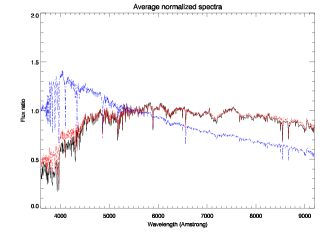
Figure 1: Normalized average spectra for NGs (black curve), S2G galaxies (red curve) and SFGs galaxies (blue curve).

Figure 2: Ratio of the normalized average spectra of NGs and S2G galaxies.

4 Metallicity of the three samples of galaxies

Three different methods have been used to estimate the metallicity of the interstellar matter and stellar populations in the central regions of galaxies of the three samples here considered. For Seyfert 2 galaxies, a photoionization model for the gas in the narrow line region of the AGN ([Vaona (2009)]) has been employed, while the content of metals of central regions of SFs and normal galaxies has been evaluated using two empirical techniques, the P method ([Pilyugin & Thuan (2005)]) and the $Mg_{2}$ index method ([Bender et al. (1993)]) respectively. The last method, namely the empirical correlation between the $Mg_{2}$ index and the metallicity, has been employed also to estimate the metallicity of S2 and SFs galaxies and compared with the metallicity provided by the other methods. In both cases, the circumnuclear stellar populations have been reconstructed using STARLIGHT. In the following sections these methods and the results of their application to the galaxy samples considered will be described.

4.1 Photoionization models

There are so many physical processes involved in the ionized gas emitting region of AGNs that building a model able to reproduce the observed spectrum is a great challenge. Following ([Netzer (2008)]), there are five main aspects to be taken into account for a correct modeling of the ionized gas physical processes: photoionization and radiative recombination, thermal balance, ionizing spectrum, gas chemical composition and clouds and/or filaments distribution. In the thermal balance we find the mechanical heating and the role of dust which is always present in the NLRs. We have excluded from our analysis the gas kinematics and winds and gas confinement mechanisms. A code such as CLOUDY [Ferland et al. (1998)] is able to solve numerically the ionization and thermal structure of a single cloud so it can be used to explore different parameters values, to build more sophisticated models such as composite models with more clouds and/or different geometries and time-dependent models. CLOUDY works with two defaults geometries, open and close respectively. The first one is based on simple photoionization field through a plane parallel slab with a defined ionized column density, while in the second case the gas is distributed all around the source. The models were made using CLOUDY code version $06.02$ [Ferland et al. (1998)]. We have assumed open geometry for all models. Once the ionizing spectrum is defined (no-thermal power-law in our case) the input parameters are the density $N_{e}/cm^{-3}$, the ionized column density $N_{c}(H^{+})/cm^{-2}$, the ionization parameter $U$ and the metal abundances,$Z/Z_{\odot}$. The ionization parameter expresses the level of ionization of photoionized gas and is proportional to the ratio of the ionizing photon density over the gas density according to the relation:

$$U=\frac{Q(H)}{4\pi r^{2}cN_{H}}$$ (4)

where c, the speed of light, is introduced to make U dimensionless. We built two kinds of photoionization models: single cloud models and composite models, the latter being based on a combination of two different single-cloud models. In the literature two fundamental approaches regarding composite models can be found: a dense cloud inside a medium with low density ([Binette et al. (1996)], or combining separately two clouds ([Komossa & Schulz (1997)]). The evaluation of the model parameters on a grid of models is the only realistic way to compare a great number of observed spectra to the models. Since our aim is to define the mean physical parameters which characterize the NLRs using spectra in the visible range, a particular attention is put on the metallicity because this parameter is important in the investigation of the nature of gas and its origin. We have generated a great number of models in order to fit all the observed lines. The well known and useful method of the line ratio diagrams employs few lines and so has limited separation power, so that if we reproduce all the measured lines the line ratio diagrams are automatically satisfied by a large number of models. In these cases, parameters values are obtained by averaging the different models. Another important result obtained by this method is the extension toward the ultraviolet (UV) and near infrared (NIR) wavelengths of the electromagnetic spectrum. A $\chi^{2}$ test has been employed to compare the models with the observed fluxes.

4.1.1 One cloud models and the input parameters

In order to explore the 5-dimensional parameter space we built, a set of single cloud models with the values for the parameters reported in Table 1. The ionizing spectra were assumed to be power-laws with $\nu^{\alpha}$ in the range $10$ $\mu$$m$ - $50$$Kev$, a cut-off at low energies ($\nu^{5/2}$) and a cut-off at high energies ($\nu^{-2}$). This choice is in agreement with the results showed in ([Komossa & Schulz (1997)]) and ([Groves et al. (2004)]), and supported by X band observations (see [Mainieri et al. (2007)]). In order to assure consistency, the column density values were checked and the simulation was interrupted when the number of transmitted ionizing photons was below $1$%; otherwise, the simulation stops when the final temperature reaches $4000K$. The basic model is summarized in Figure 3: the ionizing photons cross a slab with a fixed density, column density and dust to gas ratio (D/G) (the distance of the source is not required as a free parameter since the ionization parameter is fixed). Then the intrinsic spectrum is calculated using CLOUDY: the calculation stops when either the fixed required column density has been achieved or the temperature in the simulation has fallen below $4000$K. We assume that the intrinsic spectrum is reddened by the ISM, so when the models are compared to the observed spectra it is necessary to correct for extinction.

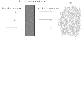
Figure 3: Basic scheme of the photoionization models.

Table 1: Input parameter values. Note that $U$, $N_{e}$ and $N_{c}(H+)$ values are reported in logarithmic notation.

$Z/Z\sun$	$\alpha$	$U$	$N_{e}$ $cm^{-3}$	$N_{c}(H+)$ $cm^{-3}$
0.5	-1.9	-3.6	1	19
1	-1.6	-3.2	1.5	19.4
1.5	-1.3	-2.8	2	19.8
2	-1	-2.4	2.5	20.2
2.5		-2	3	20.6
3		-1.6	3.5	21
3.5			4	21.4
				21.8
				22.2

4.1.2 Set of chemical abundances

The metallicity in HII regions and in star-forming galaxies may be determined by direct methods ([Aller et al. (1984)]), measuring the line flux ratios, once the temperature is determined, or through empirical but well tested metallicity sensitive calibrations ([Pilyugin & Thuan (2005)]), when it is not possible to measure directly the abundances (high metallicity or low excitation cases). In the stellar photoionization case, the ionization structure is known and so it is possible to obtain the total abundances by measuring the ionic abundances using the ionization correction factors method (see ([Mathis & Rosa (1991)]) and references therein). In the AGN, the situation is more difficult to handle since, when the ionizing spectrum is a no-thermal power-law, the ionization structure is very complex: the partial ionized region is so large so that different ionization states are mixed and taking into account the ionic abundances making up the total abundances gets quite complicated. In this case, direct methods are not possible and the empirical calibrations are obtained only by models. The choice of the sets of chemical abundances a critical step in the creation of the models because they are critically linked to another fundamental aspect of the simulations, i.e. the role of the dust and its composition. Once a reference sample of different abundances is assumed (usually, the solar set of values), a law describing the change in the chemical composition and that will be used for the exploration of different metallicities, is required. The observations of the ionized gas chemical abundances in HII regions and starburst galaxies show that all the elements, except nitrogen and helium, in first approximation are found in equal proportions. As usual, in the HII regions the metallicity is expressed in terms of oxygen abundance while in the visible spectra it is possible to measure three different ionization states and oxygen is the most abundant element after hydrogen and helium. Then, we can assume that all the elements scale directly with the oxygen abundance, except for nitrogen and helium that must be treated separately. The nitrogen abundance, as well as helium, must be corrected for secondary production [Vila Costas & Edmunds (1993)].

$$\frac{N}{H}=\frac{O}{H}[10^{-1.6}+10^{2.37+log(O/H)}].$$ (5)

$$\frac{He}{H}=0.0737+0.0293\frac{Z}{Z_{\odot}}$$ (6)

The composition and quantity of dust are also sources of uncertainties. The set of abundances needs to take into account both gas and dust composition in order to maintain the total assumed element abundances. As for the abundances of the elements, whose reference values are assumed to be similar to the solar values, the default values of abundance and composition for dust are taken from the Galactic interstellar matter (ISM). Chosen the features of the dust, the abundances of the gas component are calculated by subtracting the dust abundances from the total. With the exception of the noble gases, all abundances must be corrected for depletion into dust. This correction corresponds to a variation in the abundances of elements in gaseous form. The determination of these corrections is a main issue of modeling since it is only possible to make assumptions based on the observed properties of the Galactic ISM. It is reasonable to suppose an increase of dust with metallicity because at a metallicity increase corresponds an increment of the refracting elements. Another important assumption regards the dust to gas ratio value (D/G thereafter). By changing the relative internal dust content as a function of the metallicity, the depletion factors must also be changed, and a method to estimate the depletion factors with the variation of the dust content is presented in ([Binette et al. (1993)]). In any case, some assumptions for the D/G and the variation of the dust with the metallicity are necessary. It seems that the depletion into grains could be constant in many directions of the Galaxy (see ([Vladilo (2002)])), so we adopted the depletion factors reported in ([Groves et al. (2006)]) as reference values and a linear law for the scaling of the dust abundance with the metallicity. Using the conventional logarithmic notation, the relation between depletion factor and gas abundance is given by the formula:

$$depl(X)=log(X/H)_{gas}-log(X/H)_{tot}$$ (7)

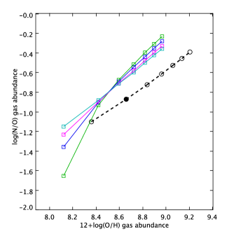
Figure 4: N/O vs O abundance, black dashed line total abundances, filled black circle the Sun abundances, colored lines: pale blue D/G=1.00, cyan D/G=0.75, blue D/G=0.50, green D/G=0.25

In this work, it is assumed $log(X/O)=$cost for all chemical elements, with the exception of N and He. For these elements we follow ([Groves et al. (2004)]) and ([groves06]) by employing a linear combination of the primary and secondary components of Nitrogen with the requirement of matching the adopted solar abundance patterns ([Asplund et al. (2005)]) (Table 2). In the models, $4$ D/G values were used in units of the ISM D/G = $0.25$, $0.50$, $0.75$, $1.00$. For each D/G value, we defined seven sets of chemical abundances, using the solar oxygen abundance as reference: $Z/Z_{\odot}$=$0.5$; $1$; $1.5$; $2$; $2.5$; $3$; $3.5$. We focused our attention on the high metallicity levels because nuclear gas and Seyfert galaxies very rarely present sub-solar metallicities ([Groves et al. (2006)]). For each adopted D/G we changed the depletion factors set in order to retain the total abundances. The set of depletion factors is constant for each assumed D/G value with the exception of nitrogen because of the secondary production. The nitrogen depletion factor must change with the metallicity because, in agreement with our assumptions, if the dust increases with the metallicity there must be an excess of nitrogen in gas form due to the formula 5. The Nitrogen may be depleted in the carbonaceous grains: the involved functional groups are Amines (N-H, C-N), Amides (N-H), Nitriles (C,N triple bond stretch), Isocyanates (-N=C=O), Isothiocyanates (-N=C=S), Imines (R2C=N-R) and Nitro groups (-NO2 aliphatic, aromatic) [Kwok (2007)]. Excluding the ammonia (NH₃), which cannot survive in an intense ionizing field such as in the AGN case, all the mentioned compounds need their partner elements linearly increasing with the metallicity. In Table 3 the depletion factors used for D/G$=1.00$ are reported. if this assumption is correct, a great increment of nitrogen gas abundance for $Z/Z_{\odot}>1.5$ should be observed, suggesting that it is not necessary to invoke an excess of nitrogen in order to match the observed $[NII]\lambda 6584$ line intensity. In the Figure 4 there are the relations between $log(N/O)_{gas}$ and $12+log(O/H)_{gas}$ for each couple of D/G and $Z/Z_{\odot}$ values. For the other elements the trend is constant at a given D/G value. It is important to stress that the depletion of the elements must be taken into consideration even if the nebula is without dust, such as in radiation-pressure dominated models of ([Groves et al. (2004)]) according to which the dust is blown away by the wind. In our models, we assumed only two types of dust, graphite and silicates; their reference abundances are $[C/H]=1.22E-04$ when D/G$=1$ in the graphite and $[O/H]=1.94E-04$, $[Mg/H]=3.15E-05$, $[Si/H]=2.82E-05$, $[Fe/H]=2.70E-05$ for silicate respectively, while the distribution of their size is in the range $[0.005,0.25]$ $\mu$m. We analyzed the abundances found in many HII regions with direct methods in order to check the relation between oxygen abundance and the other elements. In ([Van Zee et al. (1998)]), ([Van Zee & Haynes (2006)]), ([Izotov & Thuan (1999)]), ([Izotov et al. (2006]) and ([Contini et al. (2002)]) a vast collection of chemical abundances were determined in $186$ $HII$ regions spanning a range of radius in $13$ spiral galaxies, $54$ supergiant H II regions in $50$ low-metallicity blue compact galaxies, $67$ $HII$ regions in $21$ dwarf irregular galaxies, $~{}310$ emission-line galaxies from the Data Release $3$ of the SDSS and a sample of $68$ UV-selected intermediate-redshift ($0\leq z\leq 0.4$) galaxies. Our set of models does not match very well with the trend seen in Figure 5, whereas there is a better fit with the samples used by ([Groves et al. (2004)]) ([Mouhcine & Contini (2002)], [Kennicutt et al. (2003)]) but the $log(N/O)$ trend is in any case overestimated when the abundances are greater than $Z_{\odot}$. In order to compare our results with those obtained by the above mentioned authors, we adopted the same solar abundances, formalism and constraints. It is apparent that the UV-galaxies have a large spread in the $log(N/O)$ values, so it could be possible that the HII regions and starburst galaxies have different sets of chemical abundances. This hypothesis could be tested by using a sample of gas abundances in nuclei of spiral galaxies to ascertain whether the adopted function is an upper limit of the real one. The final number of models models is $10390$, $9782$, $9022$ and $8207$ for D/G=$0.25$, $0.50$, $0.75$, $1.00$ respectively. The models will be rejected unless the resulting spectra are classified as Seyfert 2 spectra in the ([Veilleux & Osterbrock (1987)]) diagnostic diagrams, following the Kewley’s conditions ([Kewley et al. (2006)]), and the synthetic fluxes are in the observed ranges, following Koski’s diagrams ([Koski (1978)]).

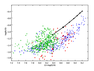
Figure 5: the log(N/O) vs 12+log(O/H): filled red circles UV galaxies, blue crosses HII regions in spiral galaxies, green crosses HII regions in blue compact galaxies, blue *** HII regions in dwarf irregular galaxies and green *** emission line galaxies, black line the adopted N/O function, the black circles show the adopted metallicity values $Z/Z\odot$, respectively 0.5, 1 (filled circle), 1.5, 2, 2.5, 3, 3.5.

Table 2: Adopted abundances and depletion factors (the depletion factor is defined as: $depl=log(X/H)_{gas}-log(X/H)_{tot}$).

el.	$log(X/H)_{\odot}$	depl	$log(X/H)_{\odot gas}$	ISM
He	-1.07	0.00	-1.07
Li	-10.95	0.00	-10.95
Be	-10.62	0.00	-10.62
B	-9.30	0.00	-9.30
C	-3.61	-0.30	-3.91	-3.91
N	-4.22	-0.30	-4.52	-4.52
O	-3.34	-0.24	-3.58	-3.71
F	-7.44	0.00	-7.44
Ne	-4.16	0.00	-4.16
Na	-5.83	-0.60	-6.43	-5.96
Mg	-4.47	-1.15	-5.62	-4.50
Al	-5.63	-1.44	-7.07	-5.65
Si	-4.49	-0.89	-5.38	-4.55
P	-6.64	0.00	-6.64
S	-4.86	-0.34	-5.20	-5.13
Cl	-6.50	-0.30	-6.80	-6.80
Ar	-5.82	0.00	-5.82
K	-6.92	0.00	-6.92
Ca	-5.68	-2.52	-8.20	-5.68
Sc	-8.95	0.00	-8.95
Ti	-7.10	0.00	-7.10
V	-8.00	0.00	-8.00
Cr	-6.36	0.00	-6.36
Mn	-6.61	0.00	-6.61
Fe	-4.55	-1.37	-5.92	-4.57
Co	-7.08	0.00	-7.08
Ni	-5.77	-1.40	-7.17	-5.79
Cu	-7.79	0.00	-7.79
Zn	-7.40	0.00	-7.40

Table 3: Nitrogen depletion factors for the ratio D/G=1.00. Relative abundances of metals are in logarithmic notation.

$Z/Z\sun$	$O/H$	$N/H$	$N/H_{gas}$	depl
0.5	-3.64	-4.75	-5.54	-0.79
1	-3.34	-4.22	-4.52	-0.3
1.5	-3.16	-3.89	-4.09	-0.19
2	-3.04	-3.66	-3.8	-0.14
2.5	-2.94	-3.48	-3.59	-0.11
3	-2.86	-3.32	-3.41	-0.09
3.5	-2.8	-3.19	-3.27	-0.08

4.1.3 Composite models

The simple single cloud model described in the previous section is( only the first step of our modeling effort since in the observed Seyfert spectra two distinct c components are usually observed, yielding high and low ionization lines. A double component model with two clouds, each accounting for either the high or the low ionization lines, can be created. We explored two kinds of composite models: Binette’s models and 2 clouds models. The first one is based on the ([Binette et al. (1996)]) work, with the only improvements represented by the exploration of a larger region of the parameter space; the second model is based on a combination of two different and independent single cloud models ([Komossa & Schulz (1997)]), as described previously. We considered all the possible combinations between two clouds with fixed power-law indexes and metallicities. The spectral lines emitted by the first and second cloud are combined by a weighted mean, where the weight is given by the product of $H_{\beta}$ luminosities ratio and the solid angle ratio ($\omega_{1}/\omega_{2}$) subtended by the clouds as seen from the source of the ionizing radiation (this ratio, called geometrical factor, is indicated by $GF$). The following steps lead to the relation which has been applied to the combined fluxes. The line luminosity is given by:

$$L=4\pi r^{2}S\omega/4\pi$$ (8)

where $r$ is the inner radius of the nebula, $\omega/4\pi$ is the covering factor, $S$ the emission line intensity ($erg$ $s^{-1}$ $cm^{-2}$). Then:

$$L=4\pi d^{2}F=4\pi r^{2}S\omega/4\pi$$ (9)

where $F$ is the observed flux ($erg$ $s^{-1}$ $cm^{-2}$), $d$ is the distance of the source. Defining the density of ionizing photons ($s^{-1}$ $cm^{-2}$) as:

$$\phi(H^{0})=Q(H^{0})/4\pi r^{2}$$ (10)

where $Q(H^{0})$ is the number of ionizing photons emitted from the source in a second and the ionization parameter as

$$U=\phi(H^{0})/n_{H}c$$ (11)

If there are two clouds:

$$U_{1}/U_{2}=r_{2}^{2}n_{2}/r_{1}^{2}n_{1}\Rightarrow r_{2}^{2}/r_{1}^{2}=U_{1}n_{1}/U_{2}n_{2}$$ (12)

and, as a consequence:

$$L_{2}/L_{1}=4\pi d^{2}F_{2}/4\pi d^{2}F_{1}=F_{2}/F_{1}$$ (13)

Then:

$$F_{2}/F_{1}=U_{1}n_{1}S_{2}\omega_{2}/U_{2}n_{2}S_{1}\omega_{1}$$ (14)

in terms of $H_{\beta}$ this ratio can be written as:

$$F_{2}(H\beta)/F_{1}(H\beta)=GF\cdot L_{2}^{{}^{\prime}}(H\beta)/L_{1}^{{}^{\prime}}(H\beta)$$ (15)

where $L_{2}^{{}^{\prime}}$($H_{\beta}$)/$L_{1}^{{}^{\prime}}$($H_{\beta}$) is the $H_{\beta}$ luminosity ratio if $\omega_{2}=\omega_{2}$. These quantities are calculated by CLOUDY for each model. If we want to find the emission line intensity $I_{\lambda}$ relative to $H_{\beta}$ then:

$$I_{\lambda}=\frac{(F_{\lambda})_{2}+(F_{\lambda})_{1}}{F_{tot}(H\beta)}$$ (16)

where $F_{tot}(H\beta)$ is the total observed flux, and rearranging the terms we obtain:

$$I_{\lambda}=\frac{(I_{\lambda})_{2}+\frac{F(H\beta)_{1}}{F(H\beta)_{2}}(I_{\lambda})_{1}}{1+\frac{F(H\beta)_{1}}{F(H\beta)_{2}}}$$ (17)

and finally:

$$I_{\lambda}=\frac{(I_{\lambda})_{2}+\frac{L_{2}^{{}^{\prime}}(H\beta)}{L_{1}^{{}^{\prime}}(H\beta)}\cdot GF\cdot(I_{\lambda})_{1}}{1+\frac{L_{2}^{{}^{\prime}}(H\beta)}{L_{1}^{{}^{\prime}}(H\beta)}\cdot GF}$$ (18)

If $GF$ goes to zero only the second cloud is visible; on the contrary, if $GF$ goes to infinity, only the first cloud is visible. Five values for $GF$ have been used ($0.25$, $0.5$, $1$, $2$ and $4$), so that each couple of models provides five new synthetical spectra.The total number of models obtained with the constrains on D/G, $\alpha$, $Z/Z_{\odot}$ fixed for each couple and after imposing the Kewley and Koski conditions, is about $9\cdot 10^{6}$.

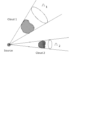
Figure 6: 2 clouds model, $\omega_{1}$ and $\omega_{2}$ are the solid angles subtended by the clouds.

4.2 Comparison of models with observations

We have compared all the measured lines coming from the observations with the synthetic data provided by the models. Our goal is to reproduce as efficiently as possible the observed spectra with the aim of determining the most realistic set of input parameters. In ([Oliva et al. (1999)]), the authors proposed a new method for deriving abundances in the AGN narrow line region (NLR), consisting in a selection of ”good’” models from a great sample (they used $27000$ models) which is capable of fairly reproducing the observed line spectra, and then slightly modifying the chemical abundances in order to determine the best estimates of the metallicity of the AGN. The very large number of synthetical spectra we have produced has been employed to determine the set of models yielding the most similar synthetic spectral features to each observed spectrum with a $\chi^{2}$ test. In this case, the $\chi^{2}$ is given by:

$$\chi^{2}=\sum_{i}(F_{\lambda_{obs}}-F_{\lambda_{C}})^{2}_{i}/(\sigma_{i})^{2}$$ (19)

where $F_{\lambda_{obs}}-F_{\lambda_{C}}$ is the difference between the observed flux and CLOUDY flux, and $\sigma_{i}$ the error associated to the i-th line. The most probable set of input parameters can be therefore determined for each observed spectrum. The comparison has been carried out taking into account the synthetical lines which are foreseen to be visible in the observed spectrum, since these lines would be detectable ($S/N>3$ ratio) in the observed spectrum. Lines below the $S/N$ value of the observed spectrum or not visible are excluded from the analysis. Two further parameters considered in the models are the reddening (Av) and the scale factor $F(H_{\beta})$. The $\chi^{2}$ test is performed using the measured fluxes not corrected by reddening while the flux models are reddened in order to achieve the observed $F(H_{\alpha})/F_{(H\beta)}$ ratio. Since we have not corrected for the extinction using a fixed value, even if close to $3.1$, many models show a significantly different value. Av is calculated applying the relation in ([Cardelli et al. (1989)]):

$$Av=7.22\cdotp\left[log\left(\frac{F(H\alpha)}{F(H\beta)}\right)_{o}-log\left(\frac{F(H\alpha)}{F(H\beta)}\right)_{C}\right]$$ (20)

Nine different values of $F(H_{\alpha})/F(H_{\beta})$, obtained combining $F(H_{\alpha})\pm\Delta F(H_{\alpha})$ with $F(H_{\beta})\pm\Delta F(H_{\beta})$ (writing in compact form the fluxes $F_{\alpha}/F_{\beta}$, $(F_{\alpha}+\Delta F_{\alpha})/F_{\beta})$, $F_{\alpha}/(F_{\beta}-\Delta F_{\beta})$ and so on), have been adopted. Then the mean ($\langle F_{\alpha}/F_{\beta}\rangle$) and the root mean square ($\sigma$) of the ratios are calculated, taking into account all the values within the range $-\sigma<\langle F_{\alpha}/F_{\beta}\rangle<\sigma$, giving as a result a positive Av value. For each model up to $9$ different synthetical spectra have been calculated. The scale factor allows us to compare directly the reddened model with the observed spectrum. Relative fluxes would have increased relative errors because of the propagation. The accepted model have to satisfy a predetermined significance level, suggested by the analysis of the reduced $\chi^{2}$ distribution and given by:

$$\chi^{2}/dof=\chi^{2}/(nr-np)$$ (21)

where ”dof” stands for degree of freedom, ”nr” is the number of measured lines and ”np” the number of parameters used in the models. The minimal number of dof necessary in order to decide the acceptability level is given by the number of measured lines minus the number of parameters used in the models. In order to consider the model a good approximation of the observed spectrum, the $\chi^{2}/dof$ distribution is required to be similar to a gaussian distribution peaked on $1$. If the peak is located at values $<<1$ there is an overestimation in the fitting, presumably caused by the fact that very large error bars fit very well not significant set of parameters of the model. On the other hand, if the peak is placed at values $>>1$, the models cannot reproduce the observed spectra or the errors are too small. The significance level has been fixed, after several tests, between $5\%$ and $10\%$ and the assumed flux errors at $2\sigma$ level. The best fit models are associated to the minimum $\chi^{2}$ value, indicated with ($\chi^{2}_{min}$), with the assumption that if a model is accepted, all the models falling within the assumed confidence region are considered as acceptable as well. This condition can be expressed as:

$$\chi^{2}-\chi^{2}_{min}<A$$ (22)

where A is the value selected for a given probability [Mollá & Hardy (2002)] ($25\%$ level of confidence is adopted in this work). For each fitted spectrum there is a group of accepted models; the best values of the parameters are evaluated by averaging the single values over all the accepted models. In this analysis, $7$ free parameters for the single cloud models (SC) have been considered. As a consequence, a minimum number of measured lines equal to $7$ and $11$ to fit such models is required, while at least $12$ measured lines and $7$ parameters for Binette’s models. About $50\%$ of the spectra shows less than $12$ measured lines, meaning that the 2C models can be compared to only the 50% of the original sample of galaxies but with the great advantage of considering only the higher S/N spectra. A spectrum with a low number of measured lines has usually low S/N, i.e. then big errors on the measured spectral lines, so, even though it is easier to fit the models with different parameters, these fits have little or no scientific validity.

4.2.1 The test

In order to compare the different kinds of models, the spectra are splitted into two groups, namely spectra with $nr\geq 12$ and spectra with $nr<12$. Since the D/G ratio is not considered a parameter of the model, the models with different D/G values will be treated separately. Such classification leads to four families of models, one for each D/G value. The number of input parameters for each kind of model are summarized in Table 4.

Table 4: The input parameters of the simulations for single cloud, double clouds and Binette’s models.

Parameter	SC	2C	Binette
power-law index, $\alpha$	yes	yes	yes
metallicity, $Z/Z_{\odot}$	yes	yes	yes
density, Ne	yes	yes	fixed
column density, Nc(H+)	yes	yes	yes
ionization parameter, U	yes	yes	yes
density 2nd cloud, Ne2	no	yes	fixed
column density 2nd cloud, Nc(H+)2	no	yes	calculated
ionization parameter 2nd cloud, U2	no	yes	calculated
geometrical factor, Gf	no	yes	yes
Reddening, Av	yes	yes	yes
Scale factor, F(Hβ)	yes	yes	yes
number of parameters	7	11	7

4.2.2 Seyfert 2

On a total of $2153$, $1141$ spectra have $nr<12$ and the remaining $nr\geq 12$. For this reason, the comparison between SC and 2C models will be done only over $1012$ spectra. In Table 5 the number of fitted spectra for each D/G value is reported; in more details, the first column contains the D/G value, second to fourth columns contain the fitted spectra with SC models and the last column the fitted spectra with 2C models. The total percentage of spectra which passed the test are $\sim 65\%$ and $\sim 50\%$ for the SC and 2C models respectively. The percentage of spectra successfully fitted with $nr<12$ is $80\%$, while $\sim 45\%$ is the fraction of spectra fitted with $nr\geq 12$. Both two 2C models accounts for only $50\%$ of the spectra fitted, since this work was carried out with the goal of achieving the best fitting and not the maximum number of spectra fitted.

Table 5: Number of fitted spectra.

D/G	SC	SC $nr<12$	SC $nr\geq 12$	2C
0.25	1249/2153	853/1141	396/1012	404/1012
0.50	1375/2153	912/1141	463/1012	486/1012
0.75	1445/2153	930/1141	515/1012	554/1012
1.00	1426/2153	939/1141	487/1012	561/1012

The $\chi^{2}/dof$ distributions are shown in figure 7. The distributions of the SC models are slightly skewed toward lower values for the D/G=$1$ and D/G=$0.75$ models, while the 2C models show tails for larger values even if their overall shapes are more regular. The significant difference between the models is evident comparing the distribution of absolute $\chi^{2}$, since this statistics represents the goodness of the overall fitting procedure (the input model parameters, the choice of the significance level and errors) and it is possible to discriminate between two models which are able to fit the same spectrum by looking at the $\chi^{2}$ value.

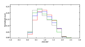
Figure 7: $\chi^{2}/dof$ distribution for SC models, up, and 2C models, down, and the different D/G values, red $0.25$, blue $0.50$, green $0.75$ and grey $1.00$.

The cumulative distributions (Figure 8) of $\chi^{2}/dof$ show clearly the great difference in the obtained fits between the two kinds of models used in this work. Within each type of models, the D/G value yielding the minimum $\chi^{2}$ values is $1$ even if the difference is not significative, while the larger overall number of fitted spectra is obtained with D/G$=0.75\div 1$. More interesting is the comparison of $\chi^{2}$ between the matched fitted spectra with single and 2C models. For each D/G value (starting from $0.25$) there are respectively $289$, $356$, $410$ and $396$ shared spectra, whose $\chi^{2}$ distributions are dramatically different. The differences can be appreciated looking at the cumulative distributions (Figure 9): spectra having good S/N are best fitted using 2C models. Many measured lines and much greater number of spectra could be fitted increasing the parameter resolution, in particular for the power-law index and the ionization parameter, at the cost of a much heavier computational load.

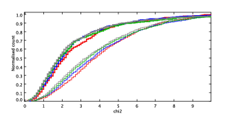
Figure 8: $\chi^{2}$ cumulative distribution for SC models, thin lines, and 2C models, thick lines.

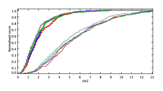
Figure 9: $\chi^{2}$ cumulative distribution for shared fitted spectra with the usual meaning of the symbols.

Table 6 contains the percentage of failures for each measured line of the observed spectra. The data show again that the 2C models fit more efficiently all the lines. Anyway, these results should be cautiously handled since the percentage of successful fits are calculated averaging over few spectra, so that a single measure could modify drastically the result (in particular for the $[ArIV]$ and $[FeVII]$ lines). The lines mostly affected by this kind of issue are $[NI]5200$, $[FeVII]5721,6087$, $HeI5876$ and $[ArIII]7135$.

Table 6: Percentage of line failures for single cloud and double cloud models.

	SC				2C
line	0.25	0.50	0.75	1.00	0.25	0.50	0.75	1.00
$[OII]$3727	6	6	7	5	3	2	2	1
$[NeIII]$3869	2	2	1	1	2	0	0	3
$[NeIII]$3968	1	1	2	3	5	2	1	1
$[SII]$4074	8	18	18	25	0	0	0	0
$H_{\gamma}$4340	0	1	1	1	0	0	0	0
$[OIII]$4363	10	0	7	8	3	6	6	8
HeII4686	2	1	1	3	0	1	0	0
$[ArIV]$4711	0	0	0	0	0	0	0	0
$[ArIV]$4740	33	25	25	20	0	0	0	0
$H_{\beta}$4861	0	0	0	0	0	0	0	0
$[OIII]$4959	0	0	0	0	0	0	0	0
$[OIII]$5007	2	3	3	3	0	0	0	0
$[NI]$5200	67	62	59	57	34	29	32	34
$[FeVII]$5721	50	60	67	67	14	10	30	33
HeI5876	19	17	16	15	8	10	9	11
$[FeVII]$6087	62	61	66	63	9	15	15	65
$[OI]$6300	7	6	7	6	2	3	5	5
$[OI]$6363	2	1	1	1	0	0	1	0
$[NII]$6548	0	0	0	0	0	0	0	0
$H_{\alpha}$6563	0	0	0	0	0	0	0	0
$[NII]$6584	2	3	4	5	0	0	0	0
$[SII]$6716	2	3	3	4	0	0	1	1
$[SII]$6731	4	4	4	4	8	6	4	1
$[ArIII]$7135	7	11	16	22	3	8	26	27
$[OII]$7325	0	0	0	0	0	0	0	10

4.2.3 Metallicities of Seyfert 2 galaxies

In Table 7 are summarized all the mean values of the parameters with their root mean square, $\sigma$, respectively for the single cloud and 2C models. The power-law index $\alpha$ decreases to $-1.8$ with the increasing of the D/G ratio, probably because of the decreasing gas metallicity content (a large fraction of metals is depleted into grains). In fact, a low metallicity of the gas implies a much slower cooling and a weaker ionizing spectrum is necessary to obtain the same degree of ionization. The total metallicity is well defined in all models with negligible scatter; $1.5\div 2.5$ $Z/Z_{\odot}$ is the range of the fitted values with the SC models while for the 2C model the estimate obtained is $1.0\div 2.0$ $Z/Z_{\odot}$. The high metallicity of the gas indicates that the AGN fuel is evolved material, which, in turn, supports the idea that the gas has a local origin in the vast majority of the observed Seyfert 2 galaxies. The densities are in agreement with the measured values: SC and SC models produce the same values of densities, both very similar to the measured sulfur density.

Table 7: Parameters output

One cloud models	$0.25$		$0.50$		$0.75$		$1.00$
Parameter	mean	$\sigma$	mean	$\sigma$	mean	$\sigma$	mean	$\sigma$
$\alpha$	-1.5	0.3	-1.6	0.3	-1.7	0.3	-1.8	0.3
$Z/Z_{\odot}$	2.0	0.6	1.9	0.6	1.9	0.5	1.8	0.5
$log(Ne)$	2.3	0.7	2.3	0.7	2.2	0.6	2.1	0.7
$log(Nc(H+))$	20.5	0.7	20.3	0.6	20.0	0.5	19.9	0.4
U	-3.1	0.2	-3.1	0.2	-3.0	0.2	-3.0	0.3
Av	1.4	0.6	1.5	0.6	1.5	0.6	1.6	0.6
2C models
$\alpha$	-1.3	0.3	-1.4	0.3	-1.6	0.3	-1.8	0.3
$Z/Z_{\odot}$	1.6	0.5	1.7	0.4	1.7	0.4	1.7	0.4
$log(Ne)$	2.2	0.8	2.2	0.8	2.1	0.7	2.2	0.8
$log(Nc(H+))$	20.2	0.4	20.2	0.4	20.2	0.4	20.2	0.4
U	-2.7	0.4	-2.6	0.4	-2.6	0.4	-2.5	0.4
$log(Ne)_{2}$	3.0	0.9	2.8	0.9	2.7	0.9	2.5	0.8
$log(Nc(H+))_{2}$	19.7	0.4	19.7	0.3	19.7	0.3	19.7	0.3
U2	-3.3	0.2	-3.3	0.2	-3.3	0.2	-3.3	0.3
Av	1.2	0.4	1.2	0.4	1.3	0.4	1.4	0.4

The column densities are very similar in the SC models and in the first cloud of the 2C models, while the second cloud of the latter model has a lower column density and a lower ionization parameter too, which allows us to treat such cloud as a ionization bounded case. The ionization parameter in the SC models is almost constant for different D/G values: $log(U)=-3$. In the 2C the high ionization cloud shows a little variation in the ionization parameter with respect to D/G values, the mean value being $log(U)=-2.6$, while a very similar value is found for the low ionization cloud ($log(U)=-3.3$). In general, the amount of ionization in the SC models is intermediate between the values found in the first and second clouds of the 2C models. Another result, which can be explained with an increasing dust content, is the increase of the absorption Av with D/G. There is an average difference of $0.2$ mag between the SC and 2C models. In Figure 10 the values of the Av found by models for all the fitted spectra and obtained with all the models are shown against the Av values estimated by Balmer decrement. The Av models appear to be slightly larger then the estimated values for both SC and 2C models. This effect can be explained by the fact that the $H_{\alpha}/H_{\beta}$ ratio obtained by CLOUDY, in the vast majority of cases, is significantly lower than the canonical value of $3.1$.

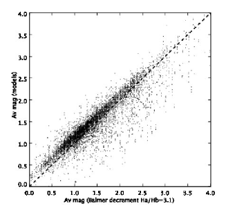
Figure 10: Comparison between the observed values of the absorption Av and the values produced by CLOUDY.

The temperatures obtained by the models are shown in Table 8. The $[OII]$ and $[SII]$ temperatures values are consistent with those measured by RO2 and RS2t ratios, while the $[OIII]$ temperature is lower than the measured one but nonetheless consistent with the photoionization case.

Table 8: Model temperatures for the observed and simulated spectral lines in single cloud and double clouds models.

	$0.25$		$0.50$		$0.75$		$1.00$
SC	Te	$\sigma$	Te	$\sigma$	Te	$\sigma$	Te	$\sigma$
${[OIII]}$	8274	1421	8522	1437	8879	1387	9374	1379
${[OII]}$	7813	1145	8142	1184	8568	1130	9136	1192
${[SII]}$	7026	1038	7282	1163	7608	1220	8021	1527
2C
${[OIII]}$	10923	3257	11172	3189	11225	2937	11535	2853
${[OII]}$	10020	3353	10390	3169	10361	2806	10736	2658
${[SII]}$	9219	3715	9560	3567	9334	3294	9759	3170
${[OIII]}_{2}$	9282	1118	9298	1085	9516	1103	9679	1140
${[OII]}_{2}$	8788	1078	8906	1016	9222	1020	9464	1006
${[SII]}_{2}$	7995	1418	8049	1353	8307	1450	8450	1480

4.3 Metallicity for star-forming galaxies

The determination of chemical abundances in the HII regions of SFs galaxies is complicated by the difficulty of reliable measures of the temperature of the HII clouds. The auroral lines, such as [OIII]4363, [SIII]6312 and [NII]5755, used to evaluate the temperature are usually weak and in low-excitation metal-rich HII regions they are often too weak to be detected. For this reason, the direct method is almost useless in the vast majority of the cases. The paper by ([Pagel et al. (1979)]) suggested that some empirical calibrations, based on collection of observations, between the nebular line fluxes could be used to derive directly the oxygen abundance or the temperature of the HII regions. In more details, the parameter defined as $R_{23}=\frac{([OII]3727+[OIII]4959,5007)}{H\beta}$ was used to directly measure the Oxygen abundances. This ratio was recalibrated using photoionization models and confirmed through other observations. Nonetheless, the comparison between the results obtained from different samples of galaxies remains very difficult because of the high heterogeneity of the model parameters and data. In all cases, the one-dimensional calibrations are systematically wrong as showed in ([Pilyugin & Thuan (2005)]). The only $R_{23}$ index does not remove all the degenerations, so a more general two-dimensional parametric calibration, called the P-method, was proposed ([Pilyugin & Thuan (2005)]), introducing a new parameter, called the excitation parameter and defined as:

$$P_{23}=\frac{([OIII]4959,5007)}{([OII]3727+[OIII]4595,5007)}$$ (23)

From a collection of high precision measurements of 700 HII regions, in ([Pilyugin & Thuan (2005)]) the authors revised the P-index calibration proposing two different functional forms for the upper branch and lower branch in the plane $R_{23}$ vs $\log{O/H}$ respectively. For the upper branch:

$$12+\log{O/H}=$$

$$\frac{(R_{23}+726.1+842.2\cdot P+337.5\cdot P^{2})}{(85.96+82.76\cdot P+43.98\cdot P^{2}+1.793\cdot R_{23})}$$

These relations can be used to determine the Oxygen abundances of the HII regions in SF galaxies and remove the degeneracies, since the P-index increases from left to right in the figure 11.

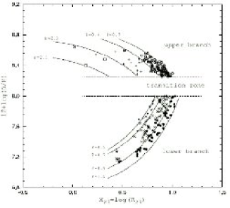
Figure 11: Family of curves in the $(R_{23},\log{O/H})$ plane labeled by different values of the excitation parameter $P$, superimposed with data from different observations. The high-metallicity HII regions with $0.0<P<0.3$ are shown as opens squares, those with $0.3<P<0.6$ as plus sign and those with $0.6<P<0.9$ as open circles. The low-metallicity HII regions with $0.5<P<0.7$ are shown as filled triangles, those with $0.7<P<0.9$ as crosses and those with $0.9<P<1.0$ as filled circles.

4.3.1 Our sample

Applying this procedure, we have found that our sample of SFs galaxies has P values in the range [0.1-0.9], consistent with the upper branch sequence and that the sources are in the transition zone 12. At the same time, the estimated Oxygen abundance of our sample is in the range [7.9-8.4]. Assuming the oxygen solar abundance of $\frac{N(O)}{N(H)}=4.5710^{-4}$ ([Asplund et al. (2005)]), the gas in this sample of galaxies has a sub-solar abundance. If the metal abundances scale with the oxygen abundance, how it is usually assumed, the gas metallicity is between 0.2 and 0.5 $Z_{\sun}$ in figure 12. It needs to be stressed that these determinations of the metal abundances take into account only the gas component and that, in order to achieve the real metallicity, dust composition has to be carefully modeled and considered. Assuming that the ISM has solar abundance, about $40\%$ of the oxygen resides in silicate grains, implying that $\frac{N(O)}{N(H)}=1.9410^{-4}$ oxygen atoms per hydrogen atom are in dust form ([Groves et al. (2006)]). Even if there is an increase in the oxygen abundance, the metallicity is in any case sub-solar or solar (the estimated value represents an upper limit because the dust content, usually, increases with the metallicity).

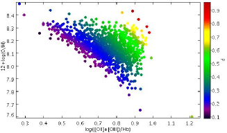
Figure 12: The star-forming galaxies of the sample used in this work in the $(R_{23},\log{O/H})$. These galaxies have excitation parameter $P$ in the interval $[0.1,0.9]$, values that are consistent with their location in the upper branch sequence of the plot.

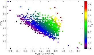
Figure 13: Same plot as before, with the assumption that total metallicity scales linearly with the Oxygen abundance. In this case, the SFs galaxies of our sample have metallicity between $0.2\cdot Z_{\sum}$ and $0.5\cdot Z_{\sun}$

5 Metallicity from stellar population synthesis

The global relationship between the stellar populations and structural properties of hot galaxies has been studied in ([Bender et al. (1993)]) using two different measures of the global stellar population, namely the $Mg_{2}$ index and the $(B-V)_{0}$ colour. The $Mg_{2}$ index, introduced in ([Faber et al. (1977)]), is defined as the the difference in magnitude between the instrumental flux in a window $F_{2}=[5156.0,5197.25]\AA$ centered on the Magnesium spectral feature and the pseudo-continuum interpolated from two windows, $F_{1}=[4897.0,4958.25]\AA$ and $F_{3}=[5303.0,5366.75]\AA$ at the blue and red sides respectively:

$$Mg_{2}=\frac{F_{2}}{F_{1}+0.61(F_{3}-F_{1})}$$ (24)

Using population synthesis models of various authors, the relation between the $Mg_{2}$ index and the central velocity dispersion $\sigma_{0}$ can be translated in an approximate relation between the same spectroscopic index and the age and metallicity of the stellar population:

$$\log{Mg_{2}}=0.41\cdot\log{\frac{Z}{Z_{\sun}}}+0.41\cdot\log{t}-1.00$$ (25)

where $Z$ is the metallicity, $t$ is the age measured in Gyr and the uncertainty on the coefficients is about $\pm 20\%$. This relation is relatively reliable for $-0.5<\log{(Z/Z_{\sun})}<0.3$ and $5<t<15$ (always expressed in Gyr). The age and metallicities of the stellar populations of the normal galaxies considered in our work have been determined by exploiting this relation. In turn, one of the two parameters has been derived from the fitted model of the continuum component of the spectrum obtained by STARLIGHT (whose output consist in a set of weights expressing the relative contribution of each single stellar population of given age and $Z$ to the observed spectrum); this estimate of either $Z$ or $t$ has been used to calculate the other parameter as an unknown term in the 25 relation, using as approximation of the measured values of the $Mg_{2}$ values the equivalent width of the MgI lines, retrieved from the SDSS database. Both temperature and metallicity of the stellar population could have been, in principle, derived by the only spectral models obtained by STARLIGHT, but this approach may prove to be essentially wrong due to the intrinsic limited coverage of the $(t,Z)$ plane of the library of template stellar population used by STARLIGHT to fit the continuum component of the observed spectra, since every possible final estimates of both parameters is a weighted average of age and metallicities of the stellar population contained in the template library.

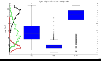
Figure 14: Distribution of mean weighted age $t$ for the three samples of galaxies considered in this work, obtained using STARLIGHT. The ”box and whisker” plots show the position of the first four quartiles of the age distribution and the outliers.

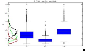
Figure 15: ”Box and whisker” plots of the distributions of the mean weighted metallicity $Z$ for the three samples of galaxies considered in this work.

The age $t$ and metallicity $Z$ distributions for all galaxies belonging to the three different samples considered in this work and derived by STARLIGHT only are shown in figures 14 and 15 as ”whisker and box” plots with, on a side, the histograms obtained from the same distributions. As expected, the normal galaxies have significantly older stellar populations than the other two samples of galaxies, among which SFs are still younger than Seyfert 2 galaxies. The metallicity distributions show that normal galaxies and Seyfert galaxies, while almost consistent from a statistical point of view, possess more evolved stellar populations than star-forming galaxies. On the other hand, the same distributions obtained using the measured values of the $Mg_{2}$ index and the relation 25 are shown in figures LABEL:mh2_t and 17 respectively. The comparison between these plots indicates that, though the relative relations between distributions of different samples of galaxies remain unchanged, stellar populations appear to be systematically younger and less metal-rich than in the case of the estimation by STARLIGHT only.

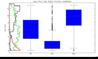
Figure 16: ”Box and whisker” plots of the distributions of the mean weighted age $t$ for the three samples of galaxies considered in this work. These estimates have been obtained using the relation 25, the mean metallicity provided by STARLIGHT and the observed Mg2 indexes of the galaxies.

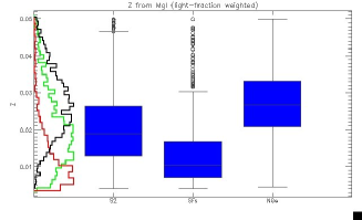
Figure 17: ”Box and whisker” plots of the distributions of the mean weighted metallicities $Z$ for the three samples of galaxies considered in this work. These estimates have been obtained using the relation 25, the mean weighted age provided by STARLIGHT and the observed Mg2 indexes of the galaxies.

6 Conclusions

In this work the metal content of the stellar and gaseous components of the central regions of galaxies has been characterized with multiple methods. Three different samples of galaxies, namely normal galaxies, star-forming galaxies and galaxies hosting an AGN (Seyfert 2), retrieved from the SDSS DR7 spectroscopic database and classified according to an original method based on spectroscopic diagnostics (see [Vaona (2009)]), have been compared. For what the nuclear stellar populations are concerned, the presence of a strong blue continuum and the absence of any 4000Å  break in the spectra of the SF galaxies are an indication of the presence, in their circumnuclear regions, of an excess of young hot blue stars compared with NG and S2G. On the contrary, the spectra of the circumnuclear regions of S2G and NG indicate quite similar conditions: a dominating stellar component of type F and a 4000Å  break in NG deeper than in S2G of a factor $\sim$1.5. This indicates that the presence of an excess of A stars in the central regions of S2G compared to NG is quite likely, suggesting that there have been in the recent past of S2 AGN slightly more star formation events than in NG. The analysis of the gas of the central regions of the Seyfert 2 galaxies has been performed using a very robust modeling of the photoionization processes occurring in gas clouds around the AGN and exploring a very large region of the model parameters space in order to reproduce realistically the observed spectra from simulation. Both single and two clouds models indicate for S2 a significantly larger metallicity than solar ($1.5\div 2.5\ Z/Z_{\odot}$ with SC models and $1.0\div 2.0\ Z/Z_{\odot}$ for the 2C models). These results support the idea that the AGN fuel is composed by evolved material and that the gas has a local origin in most of the observed Seyfert 2 galaxies. The gas metal abundances for SF galaxies have been estimated using the method of the P-index ([Pilyugin & Thuan (2005)]) and we have obtained results which clearly indicate sub-solar metal abundances (0.2 - 0.5 $Z_{\sun}$), confirming that young stars are fueled by relatively primordial and unprocessed material. The overall relations between the average age and metallicity of central stellar populations of the three different samples of galaxies here considered have been determined using the $Mg_{2}$ absorption feature as proposed by([Faber et al. (1977)]) and exploiting the spectral continuum components of observed spectra of the galaxies extracted using STARLIGHT ([Rafanelli et al. (2009)]). This analysis qualitatively confirms that Seyfert 2 galaxies have young low-metallicity circumnuclear stellar populations feeding in a metal-rich environment where gas clouds are composed of rather high metallicity material; on the other hand, SF galaxies have very young and primordial central stellar populations. In conclusion, the comparative study of metallic content of stars and gas in this work indicate that Seyfert 2 nuclei occur preferentially in a stellar environment composed of young stars where recent circumnuclear star formation processes were active (as witnessed by the high metallicity of gas clouds), even if there is no compelling evidence that would connect present or past star formation activity to the nature of the central engine. The two phenomena, SF and AGN activity, may therefore be not causally connected to each other or, if so, through indirect or/and not clear physical mechanisms.

References

- [Aller et al. (1984)] Aller, L. H. 1984, in ”Physics of thermal gaseous nebulae”, editor: Astrophysics and Space Science Library
- [Asplund et al. (2005)] Asplund, M., Grevesse, N & Sauval, A.J. 2005, ASPCS.
- [Bender et al. (1993)] Bender, R., Burstein, D. & Faber, S. M. 2003, AJ, 1, 411, 1531
- [Binette et al. (1993)] Binette, L. et al. 1993, ApJ, 414, 535-551
- [Binette et al. (1996)] Binette, L., et al. 1996, AAP, 312, 365-379
- [Boesgaard et al. (1998)] Boesgaard, A. M., et al. 1998, ApJ, 493, 206
- [Bruzual & Charlot (2003)] Bruzual, G., & Charlot, S. 2003, MNRAS, 344, 1000
- [Cardelli et al. (1989)] Cardelli, J. A. 1998, ApJ, 345, 245-256
- [Cid Fernandes et al. (2004)] Cid Fernandes, R., et al. 2004, ApJ, 605, 105
- [Contini et al. (2002)] Contini, T. et al. 2002, VizieR Online Data Catalogue, 733, 75
- [Faber et al. (1977)] Faber, S. M. 1977, PASP, 89, 23
- [Ferland et al. (1998)] Ferland, G. J., et al. 1998, PASP, 110, 761-778.
- [Groves et al. (2004)] Groves, B. A, et al. 2004, ApJS, 153, 9-73
- [Groves et al. (2006)] Groves, B. A, Heckman, T. M & Kauffmann, G. 2005, MNRAS, 371, 1559
- [Izotov & Thuan (1999)] Izotov, Y. I. & Thuan, T. X. 1999, ApJ, 511, 639-659
- [Izotov et al. (2006] Izotov, Y. I. et al. 2006, AAP, 448, 955-970
- [Kennicutt et al. (2003)] Kennicutt, Jr., R. C. et al. 2003, ApJ, 591, 801-820
- [Kewley et al. (2006)] Kewley, L. J., Groves, B., Kauffmann, G., & Heckman, T. 2006, MNRAS, 372, 961
- [Kwok (2007)] Kwok, S 2007, in ”Physics and chemistry of the interstellar medium”, editor: University of Science Book
- [Komossa & Schulz (1997)] Komossa, S. & Schulz, H. 1997, AAP, 323, 31-36
- [Koski (1978)] Koski, A. T. 1978, ApJ, 223, 56-73
- [Mainieri et al. (2007)] Mainieri, V., et al. 2007, ApJS, 172, 368-382
- [Mathis & Rosa (1991)] Mathis, J. S. & Rosa, M. R., 1991, AAP, 245, 625-634
- [Mollá & Hardy (2002)] Mollá, M. & Hardy, E. 2002, AJ, 123, 3055-3066
- [Mouhcine & Contini (2002)] Mouhcine, M. & Contini, T. 2002, AAP, 389, 106-114
- [Netzer (2008)] Netzer, H. 2008, NewAR, 52, 257-273
- [Pagel et al. (1979)] Pagel, B. E. J. et al. 1979, MNRAS, 189, 95
- [Pilyugin & Thuan (2005)] Pilyugin, L. S. & Thuan, T. X. 2005, ApJ, 631, 231
- [Oliva et al. (1999)] Oliva, E. et al. 1999, ApJ, 342, 87-100
- [Rafanelli et al. (2009)] Rafanelli, P., et al. 2009, NewAR, 53, 7-10, 186-190
- [Schlegel et al. (1998)] Schlegel D. J. et al. 1998, ApJ, 500, 525
- [Van Zee et al. (1998)] Van Zee, L. et al. 1998, AJ, 116, 2805-2833
- [Van Zee & Haynes (2006)] Van Zee, L. & Haynes, M. P. 2006, ApJ, 636, 214-239
- [Vaona (2009)] Vaona, L., 2009, PhD Thesis
- [Vila Costas & Edmunds (1993)] Vila Costas, M. B. & Edmunds, M. G. 1993, MNRAS, 265, 199
- [Vladilo (2002)] Vladilo, G. 2002, ApJ, 569, 295-303
- [Veilleux & Osterbrock (1987)] Veilleux, S. & Osterbrock, D. E. 1987, ApJS, 63, 295