Wave communication across regular lattices

Abstract

We propose a novel way to communicate signals in the form of waves across a $d$ - dimensional lattice. The mechanism is based on quantum search algorithms and makes it possible to both search for marked positions in a regular grid and to communicate between two (or more) points on the lattice. Remarkably, neither the sender nor the receiver needs to know the position of each other despite the fact that the signal is only exchanged between the contributing parties. This is an example of using wave interference as a resource by controlling localisation phenomena effectively. Possible experimental realisations will be discussed.

Localization phenomena in linear wave systems are closely linked to wave interference effects. Anderson localisation in disordered media is a prime example thereof still posing challenges to both theory and experiment Hu08 60 years after its discovery And58 . Recently, a new research area has emerged focusing on interference as a resource and making use of localisation phenomena in a controlled way. Prominent examples are among others time reversal imaging deR and reconstructing the Green function in terms of correlation functions Wea05 , see also TS07 . Here, information about the wave system is obtained by manipulating a seemingly ‘noisy’ signal using phase coherence. We will focus here on another class of wave localisation phenomena with counterintuitive properties, namely (quantum) search algorithms and (quantum) random walks. Wave search algorithms gained prominence with Grover’s work Gro96 demonstrating a $\sqrt{N}$ speed-up compared to a classical search within an unsorted data base of $N$ items. Even though search algorithms became an inherent part of quantum information theory NC00 , the speed-up is in effect caused by wave interference as has already been pointed out by Grover GS02 and has been implemented for a classical wave system in BLS02 . Based on ideas from quantum random walks ADZ93 ; kempe ; SJK08 , Grover’s algorithm has been generalized to spatial search algorithms on networks such as on a hypercube SKW03 ; HT09 and on regular lattices AKR05 . Experimental realisations of quantum random walks have been achieved again both using classical waves (optics) BMK99 and quantum devices XSBL08 .

Starting from wave search algorithms, we will demonstrate that localisation can be used to establish communication channels across a regular lattice with surprising properties: (i) signals can be exchanged exclusively between a source and a receiver point, where neither the sender nor the receiver know the position of each other; (ii) the signal can track a moving receiver in the network; (iii) the algorithm can be used as a searching device without the necessity to know the time of measurement, (a typical requirement for Grover’s search algorithm); (iv) the protocol can act as a sensitive switching device for wave transport through a lattice; (v) the algorithm can be effectively implemented both on a quantum computer and using classical waves only. We will first describe the set-up of the search algorithm. We then introduce a simplified model for the search and explain the wave communication protocol.

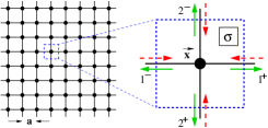
Figure 1: Regular grid with $d=2,n=8$; local scattering within a unit cell at vertex $\vec{x}$ is described by the matrix $\sigma$.

We consider wave propagation across $d$-dimensional periodic lattices of identical scatterers or periodic potentials with fixed lattice parameter $a$, see Fig. 1. It is important that the lattice has a finite number of sites $n$ along each axis with a total number $n^{d}$ of lattice sites. To simplify the calculations we will restrict ourselves to models with nearest-neighbour interaction only and consider periodic boundary conditions. The wave dynamics within each unit cell is given by a local scattering matrix $\sigma$ mapping incoming channels onto outgoing channels, see Fig. 1. ($\sigma$ is also denoted a coin matrix in the context of quantum walks). The overall wave dynamics is then given in terms of an operator $U_{0}$ mapping incoming onto outgoing wave coefficients between unit cells. We have $\mbox{dim }U_{0}=m\,n^{d}$ where $m$ denotes the number of open scattering channels within a unit cell. Furthermore, $U_{0}$ is unitary when disregarding dissipation. Stationary solutions are obtained by the condition

$$\det\left(1-{\rm e}^{{\rm i}ka}U_{0}\right)\equiv 0$$ (1)

where $k$ is the wave length and $\exp({\rm i}ka)$ is a phase shift between incoming and outgoing waves. We neglect any (in general weak) $k$ dependence of $\sigma$ and thus $U_{0}$. Note that the spectrum obtained from (1) is now periodic in $k$ with period $2\pi/a$; the eigenvalues are $k_{j,l}=(2\pi l-\theta_{j})/a,\,l\in\mathbb{N}$ , where $\theta_{j}$ are the eigenphases of $U_{0}$ with $j=1,\ldots,N$. To start with, we will consider a model consisting of a single open channel between nearby lattice sites ($m=2d$) and we assume Kirchhoff boundary conditions at each vertex. The Hilbert space is then effectively $N=2d\,n^{d}$ dimensional. This physical model captures the essence behind the effect described below.

We label incoming wave components from each unit cell as $\left|i^{\pm}\right\rangle\otimes\left|\vec{x}\right\rangle=\left|i^{\pm},\vec{x}\right\rangle$, where $\vec{x}$ specifies the vertex in position space and $i^{\pm}$, for $i=1,\dots,d$ gives the $\pm$ direction in dimension $i$. Incoming waves at vertex $\vec{x}$ are mapped onto outgoing waves by a scattering matrix $\sigma$. For Kirchhoff boundary conditions, one obtains $\sigma=2\left|s\right\rangle\left\langle s\right|-\mathbbm{1}_{2d}$ and $\left|s\right\rangle$ is the uniform distribution $\left|s\right\rangle=\frac{1}{\sqrt{2d}}\sum_{i=1}^{d}\left(\left|i^{+}\right\rangle+\left|i^{-}\right\rangle\right)$ AKR05 . Outgoing waves in direction $i^{\pm}$ are now identified with incoming waves at an adjacent vertex $\vec{x}\pm a\,\vec{e}_{i}$ where $\vec{e}_{i}$ is the unit vector in direction $i$. The local scattering processes is described in terms of a (global) scattering (or coin) matrix $C=\sigma\otimes\mathbbm{1}_{n^{d}}$. The full wave propagator (or quantum walk) $U_{0}$ is obtained from $C$ after identifying incoming and outgoing waves of adjacent unit cells accordingly. The spectrum of the unperturbed walk $U_{0}$ exhibits a band structure as shown in Fig. 2 a), here for $d=2$. (For a finite lattice, the quasi-momenta $\kappa_{x},\kappa_{y}$ are discretised according to $\kappa_{x,y}=2\pi j/(na);\,j=0\ldots n-1$.)

Following Ambainis, Kempe and Rivosh (AKR), the quantum walk $U_{0}$ acts as a search algorithm after marking a target vertex $\left|v\right\rangle$ by a modified scattering matrix $\sigma^{\prime}$ AKR05 , that is, one considers $C^{\prime}=C-\left(\sigma-\sigma^{\prime}\right)\otimes\left|v\right\rangle\left\langle v\right|$. The AKR search uses $\sigma^{\prime}=-\mathbbm{1}_{2d}$. Since $\left|s\right\rangle$ is an eigenvector of $\sigma$, we may write $U^{\prime}=U_{0}\left(1-2\left|sv\right\rangle\left\langle sv\right|\right)$, where $\left|sv\right\rangle=\left|s\right\rangle\otimes\left|v\right\rangle$. The search algorithm is initialised in the uniform state $\left|\Phi_{0}\right\rangle=1/\sqrt{N}\sum_{\vec{x}}\left|s\vec{x}\right\rangle$, and the walk $(U^{\prime})^{T}\left|\Phi_{0}\right\rangle$ localizes at $|{v}\rangle$ after $T\propto\sqrt{N}$ steps.

The AKR search can be analysed by defining a one parameter family of unitary operators HT09

$$U_{\lambda}=U_{0}+\left({\rm e}^{{\rm i}\pi\lambda}-1\right)U_{0}\left|sv\right\rangle\left\langle sv\right|;$$ (2)

one obtains $U_{0}$ for $\lambda=0$ or 2 and the AKR search for $\lambda=1$. The part of the eigenfrequency spectrum of $U_{\lambda}$ interacting with the perturbation is shown in Fig. 2 b). The spectrum is periodic in $k$ with period $2\pi/a$ independent of $\lambda$. When varying $\lambda$, a “perturber state” $|\nu_{\lambda}\rangle$ emerges which crosses the $k\mod 2\pi/a=0$ axis at $\lambda=1$. The resulting avoided crossing between the initial state $|\Phi_{0}\rangle$ and $|\nu_{\lambda}\rangle$ is shown in Fig. 2 c). Note that $|\Phi_{0}\rangle$ is the fully symmetric eigenstate of $U_{0}$ corresponding to a $d$-dimensional Bloch-vector $\vec{\kappa}=0$ of the unperturbed spectrum with eigenvalue $k\mod 2\pi/a=0$. Like in Grover’s algorithm, the quantum search $U^{\prime}=U_{\lambda=1}$ rotates the initial state $|\Phi_{0}\rangle$ into a localised state $|\nu_{\lambda}\rangle$ which has here a strong overlap with the target state $|sv\rangle$. The search time $T_{0}$ is inversely proportional to the gap at the avoided crossing $\Delta$, that is, $T_{0}\approx{\pi}/{\Delta}$.

In order to obtain an estimate for the search time $T_{0}$ as well as the efficiency of the search, that is, the matrix element $\langle sv|\nu_{\lambda}\rangle$, it is essential to find the approximately invariant two-level subspace near the crossing spanned by $|\Phi_{0}\rangle$ and $|\nu_{\lambda=1}\rangle$. The technique developed in HT09 for the hypercube has been adapted to regular grids. We will only give the result here, further details will be presented elsewhere HT09I . One finds for the normalised vector $\left|\nu_{\lambda=1}\right\rangle$

$$\left|\nu_{\lambda=1}\right\rangle = -\langle sv|v_{\lambda=1}\rangle\sqrt{\frac{2}{N}}\sum_{\vec{\kappa}\neq\vec{0}}{\rm e}^{-\frac{2\pi{\rm i}}{n}\vec{\kappa}\vec{v}}\times$$

$$\left(\frac{{\rm e}^{{\rm i}\theta_{\vec{\kappa}}}}{1-{\rm e}^{{\rm i}\theta_{\vec{\kappa}}}}\left|\Phi_{\vec{\kappa}}^{+}\right\rangle+\frac{{\rm e}^{-{\rm i}\theta_{\vec{\kappa}}}}{1-{\rm e}^{-{\rm i}\theta_{\vec{\kappa}}}}\left|\Phi_{\vec{\kappa}}^{-}\right\rangle\right),$$

where $\vec{v}$ is the position of the target vertex and $|\Phi^{\pm}_{\vec{\kappa}}\rangle$ and $\pm\theta_{\vec{\kappa}}$ are the eigenvectors and eigenphases of the unperturbed walk $U_{0}$ AKR05 . The $d$-dimensional label $\vec{\kappa}$ with $\kappa_{i}=0,\ldots,n-1$ is equivalent to the (discretised) Bloch wave number, see Fig. 2 a). The eigenphases are explicitly given as $\cos\theta_{\vec{\kappa}}=\frac{1}{d}\sum_{i=1}^{d}\cos\frac{2\pi\kappa_{i}}{n}$. The overlap-matrix element $\langle sv|\nu_{\lambda=1}\rangle$ can be estimated HT09I :

$$\langle sv|\nu_{\lambda=1}\rangle=\left\{\begin{array}[]{lcl}{\cal O}(1/\sqrt{\log N)}&\mbox{for}&d=2,\\ {\cal O}(1)&\mbox{for}&d>2.\end{array}\right.$$

Detailed expressions for the leading order coefficients for $d=2$ and 3 are given in HT09I . We find that $|\nu_{\lambda=1}\rangle$ is exponentially localised on the marked vertex $\vec{v}$; note, that the overlap of $|sv\rangle$ with a typical eigenstate of the unperturbed spectrum $|\Phi_{\kappa}\rangle$ is of the order ${\cal O}(N^{-\frac{1}{2}})\ll{\cal O}(1)$.

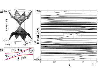
Figure 2: a) The band structure at $\lambda=0$ for $d=2$ and in the limit $n\to\infty$ with $\vec{\kappa}$, the Bloch wave numbers; b) the eigenphases of $U_{\lambda}$ for $n=11$, $d=2$; c) the avoided crossing with spectral gap $\Delta$ at $\lambda=1$ and $k\mod 2\pi/a=0$ together with the approximate eigenstates $|\nu_{\lambda}\rangle$ and $|\Phi_{0}\rangle$ (dashed lines).

Near the avoided crossing, the level dynamics can be described in terms of the two-level sub-space spanned by the orthogonal vectors $|\nu_{\lambda}\rangle$ and $|\Phi_{0}\rangle$. Writing the unitary operator $U_{\lambda}$ as $U_{\lambda}={\rm e}^{-{\rm i}H_{\lambda}}$, one obtains at $\lambda=1$ in the $\{|\Phi_{0}\rangle,|\nu_{\lambda=1}\rangle\}$ basis an effective two-dimensional Hamiltonian $H_{\lambda=1}$ of the form

$$H^{2\times 2}=\begin{pmatrix}k_{l}a&-{\rm i}\epsilon\\ {\rm i}\epsilon&k_{l}a\end{pmatrix}$$ (4)

with $k_{l}=2\pi l/a,l\in\mathbb{N}$ being the wave numbers corresponding to $\vec{\kappa}=0$ states of the unperturbed lattice and $\epsilon$ is a real and positive coupling parameter, that is,

$$\epsilon=\frac{\Delta}{2}=\langle\nu_{\lambda=1}|U_{1}|\Phi_{0}\rangle\approx\frac{2\left|\langle sv\mid\nu_{\lambda}\rangle\right|}{\sqrt{N}}+{\cal O}\left(N^{-1}\right)$$ (5)

with $\Delta$, the gap at the avoided crossing.

The start vector $(1,0)\equiv|\Phi_{0}\rangle$ is rotated into the localised state $(0,1)\equiv|\nu_{\lambda=1}\rangle$ in $T_{0}=\pi/(2\epsilon)$ steps leading to the $\sqrt{N}$ speed-up AKR05 . The whole process is $2\,T_{0}$-periodic , that is, one needs - like for Grover’s algorithm Gro96 - to know the period $T_{0}$ to perform the search. For a simulation of the search on a $31\times 31$ grid, see Fig. 3.

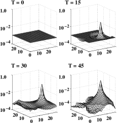
Figure 3: Probability distribution of the quantum walk on a $31\times 31$-grid up to $T=45$ time steps.

Interesting applications emerge when considering several target vertices, $\left|v^{i}\right\rangle,i=1,\ldots m$ with $m\ll N$. We now define a set of parameters $\lambda=(\lambda_{1},\ldots,\lambda_{m})$ and a search algorithm of the form

$$U_{\lambda}=U+\sum_{i=1}^{m}\left({\rm e}^{{\rm i}\pi\lambda_{i}}-1\right)U\left|sv^{i}\right\rangle\left\langle sv^{i}\right|.$$ (6)

At $\lambda=\left(1,1,\dots,1\right)$ and $ka\mod 2\pi=0$, one finds that there are $m-1$ degenerate eigenvalues and two further eigenvalues forming an avoided crossing with the degenerate subset. The corresponding set of $m+1$ eigenstates coincides in good approximation with the subspace spanned by the uniform distribution $|\Phi_{0}\rangle$ and now $m$ localised states $\left|\nu_{\lambda}^{i}\right\rangle,i=1,\ldots,m$. Each of the $\left|\nu_{\lambda}^{i}\right\rangle$ is well described by the approximation (Wave communication across regular lattices) and $\langle\nu_{\lambda}^{i}|\nu_{\lambda}^{j}\rangle\approx\delta_{ij}$. The localised states interact at the crossing predominantly via $|\Phi_{0}\rangle$ which takes on the role of a carrier state. In analogy to (4), we write a model Hamiltonian at the crossing in the basis $\{|\Phi_{0}\rangle,|\nu_{\lambda=1}^{1}\rangle,\ldots,|\nu_{\lambda=1}^{m}\rangle\}$ as

$$H^{\left(m+1\right)\times\left(m+1\right)}=\begin{pmatrix}k_{l}a&-{\rm i}\epsilon&-{\rm i}\epsilon&\dots&-{\rm i}\epsilon\\ {\rm i}\epsilon&k_{l}a&0&\dots&0\\ {\rm i}\epsilon&0&k_{l}a&\ddots&\vdots\\ \vdots&\vdots&\ddots&\ddots&0\\ {\rm i}\epsilon&0&\dots&0&k_{l}a\\ \end{pmatrix}.$$ (7)

Like for the full propagator $U_{{\lambda}=1}$, the spectrum of $H^{\left(m+1\right)\times\left(m+1\right)}$ consists of $\left(m-1\right)$ eigenvalues equal to $k_{l}a$ and two eigenvalues $k_{l}a\pm\sqrt{m}\epsilon$ with eigenvectors $|\omega^{\pm}\rangle={\rm i}/\sqrt{2m}\left(\mp{\rm i}\sqrt{m},1,\dots,1\right)^{\rm t}$. The gap between the non-degenerate levels is now $\Delta=2\sqrt{m}\epsilon$ with $\epsilon$ given in (5). Starting the search in the totally symmetric state $|\Phi_{0}\rangle$ at $\lambda=(1,\ldots,1)$, one finds that $U^{T}_{\lambda}|\Phi_{0}\rangle$ localises on all $m$ marked vertices after $T_{0}\sim\pi/2\sqrt{N/m}$ (or, for $d=2$, $T_{0}\sim\pi/2\sqrt{N/m\log N}$) steps simultaneously.

More interestingly, the quantum walk can also be used to transmit signals across the network. Such a sender-receiver configuration has to the best of our knowledge not been described before and may have interesting applications both in a quantum setting, but also for classical waves (such as microwaves, in optics or acoustics). Instead of starting the walk in the uniform state $|\Phi_{0}\rangle$, we propose to begin the walk at one of the localised states $|\nu_{\lambda}^{m}\rangle$, say. At the avoided crossing, this state can approximately be described as

$$|\nu_{\lambda}^{m}\rangle=-\frac{{\rm i}}{\sqrt{2m}}\left(|\omega^{+}\rangle+|\omega^{-}\rangle-{\rm i}\sqrt{2(m-1)}|\omega_{0}\rangle\right)$$ (8)

with $|\omega_{0}\rangle=(m(m-1))^{-1/2}(0,1\ldots,1-m)^{t}$ in the basis spanning $H^{(m+1)\times(m+1)}$; $|\omega_{0}\rangle$ is a vector in the degenerate eigenspace with eigenvalue $k_{l}a$. Applying the walk for $T_{s}=\pi/(\epsilon\sqrt{m})=2T_{0}$ steps leads to

$$U^{T_{s}}|\nu_{\lambda}^{m}\rangle = \frac{{\rm i}{\rm e}^{{\rm i}k_{l}aT_{s}}}{\sqrt{2m}}\left(|\omega^{+}\rangle+|\omega^{-}\rangle+{\rm i}\sqrt{2(m-1)}|\omega_{0}\rangle\right)$$

$$= {\rm e}^{{\rm i}k_{l}aT_{s}}\left(0,-\frac{2}{m},\ldots,-\frac{2}{m},1-\frac{2}{m}\right)^{t}.$$

This implies that a signal of intensity $4/m^{2}$ is transmitted from the sender (located at the $m$-th marked vertex) to each of the $m-1$ other marked vertices. The intensity at the sender at time $T_{s}$ is then of the order $(1-2/m)^{2}$. These findings have been verified numerically in our model. Interestingly, in the case $m=2$ with a single receiver, the signal is transmitted in full. This opens up the possibility of transferring signals directly between two points on a network where neither the sender nor the receiver know each other’s position. In addition, the sender has information about the number of receivers by recording the signal at time $T_{s}$.

The effect persists also for a continuous source at the sender position. In Fig. 4, we recorded the signal both at the sender and at the receiver. (To keep the signal finite, we added a small amount of absorption across the network). Again, without prior knowledge of the receiver’s position, the network localises at the two marked vertices, thus making it possible to actually exchange information continuously between these two points. Changing the position of the receiver leads to a sudden drop of the signal at the old receiver position and a build-up at the new position, see Fig. 4. The system is thus capable of tracking a moving receiver position! The signal speed is limited by the transfer time $T_{s}\sim\sqrt{N}$ ($T_{s}\sim\sqrt{N\ln N}$ for d=2) and thus is the speed at which the receiver can move.

The continuous sender/receiver protocol can also be used to search a marked item without knowing the search time $T_{0}$; this is a serious complication of Grover-type search algorithms when the precise number of marked items is not know (as $T_{0}$ depends on $m$). Here, we find the marked items as long as we wait for times $T\geq T_{s}$. Furthermore, the system can act as a switching device. Wave transport between two points on the grid can only be achieved, if the system is tuned to the avoided crossing. Slight detuning by for example changing the parameter $\lambda$ in (2) will quickly cut-off the signal.

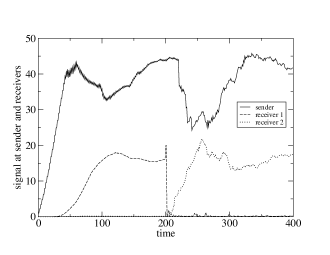
Figure 4: Sending continuously: signal at sender (full) and receivers (dashed/dotted). The response of the system to switching the position of the receiver at $T=200$ is shown. (We introduced a damping of 1% at all vertices.)

The described effects open up completely new ways of transmitting signals across regular networks. While a construction of the map $U$ is certainly feasible in a quantum setting and can be implemented efficiently on a quantum computer NC00 , an implementation using classical waves may be even more promising. For dispersionless wave dynamics and on regular lattices, the unitary matrix $U_{\lambda}$ is equivalent to a discretised version of the time dependent Green function (for times $t=a/c$ with $c$ being the wave velocity; corresponding time scales in a quantum setting would be given by the group velocity KP09 ). Indeed, localised states due to a local perturbation in a regular lattice are well known; (for example in optical crystals, see Joa08 ). We predict that the effect will occur if “defect states” created by local phase perturbations (equivalent to the perturbed coin $C^{\prime}$) are pushed into the (discretised continuum) of the band close to the fully periodic state - the $\vec{\kappa}=0$ state, see Fig. 2 a. Furthermore, the interaction between the defect states and the lattice states must be small enough to lead to avoided crossings between these two states only. We expect that a signal (such as a laser or a microwave transmitter coupled into a periodic structure at a defect position) can be transmitted and focused onto another defect in the same lattice using the described effect. The totally symmetric state $|\Phi_{0}\rangle$ acts then as a carrier state guiding the signal between the perturbations.

We thank J Keating, U Kuhl, T Monteiro, U Peschel, H-J Stöckmann and H Susanto for helpful discussions and S Gnutzmann for carefully reading the manuscript.

References

- (1) H. Hu et al, Nature Physics 4, 945 (2008) and ref. therin.
- (2) A. Anderson, Phys. Rev. 109, 1492 (1958).
- (3) J. de Rosny and M. Fink, Phys. Rev. Lett. 89, 124301 (2002).
- (4) R. L. Weaver, Sience 307, 1568 (2005).
- (5) G. Tanner and N. Søndergaard, J. Phys. A 40, R443 (2007).
- (6) L. K. Grover, Phys. Rev. Lett., 79 325 (1997).
- (7) M. A. Nielsen and I. L. Chuang, Quantum Computation and Quantum Information, (Camb. Uni. Press 2000).
- (8) L. K. Grover and A. M. Sengupta, Phys. Rev. A 65, 032319 (2002).
- (9) N. Bhattacharya, H. B. Linden van den Heuvell and R. J. C. Spreeuw, Phys. Rev. Lett. 88 137901 (2002).
- (10) Y. Aharonov, L. Davidovich and N. Zagury, Phys. Rev. A 48, 1687 (1993).
- (11) J. Kempe, Contemporary Physics, 44 307 (2003)
- (12) M. Stefanak et al, Phys. Rev. Lett. 100, 020501 (2008).
- (13) N. Shenvi, J. Kempe and K. B. Whaley, Physical Review A, 67 052307 (2003).
- (14) B. Hein and G. Tanner, J. Phys. A 42 085303 (2009).
- (15) A. Ambainis, J. Kempe and A. Rivosh, Proceedings of the 16th ACM-SIAM SODA (SIAM, Philadelphia, 2005), p. 1099.
- (16) D. Bouwmeester et al, Phys. Rev. A 61, 013410 (1999); P. L. Knight et al, Phys. Rev. A 68 020301 (R) (2003).
- (17) P. Xue et al, Phys. Rev. A 78, 042334 (2008); H. Schmitz et al, Phys. Rev. Lett. 103, 090504.
- (18) B. Hein and G. Tanner, in preparation.
- (19) J. D. Joannopoulos et al, Photonic Crystals, (Princ. Uni. Press, Princeton, 2008).
- (20) A. Kempf and R. Portugal, Phys. Rev. A 79, 052317 (2009).