The Kepler Pixel Response Function

Abstract

Kepler seeks to detect sequences of transits of Earth-size exoplanets orbiting Solar-like stars. Such transit signals are on the order of 100 ppm. The high photometric precision demanded by Kepler requires detailed knowledge of how the Kepler pixels respond to starlight during a nominal observation. This information is provided by the Kepler pixel response function (PRF), defined as the composite of Kepler’s optical point spread function, integrated spacecraft pointing jitter during a nominal cadence and other systematic effects. To provide sub-pixel resolution, the PRF is represented as a piecewise-continuous polynomial on a sub-pixel mesh. This continuous representation allows the prediction of a star’s flux value on any pixel given the star’s pixel position. The advantages and difficulties of this polynomial representation are discussed, including characterization of spatial variation in the PRF and the smoothing of discontinuities between sub-pixel polynomial patches. On-orbit super-resolution measurements of the PRF across the Kepler field of view are described. Two uses of the PRF are presented: the selection of pixels for each star that maximizes the photometric signal to noise ratio for that star, and PRF-fitted centroids which provide robust and accurate stellar positions on the CCD, primarily used for attitude and plate scale tracking. Good knowledge of the PRF has been a critical component for the successful collection of high-precision photometry by Kepler.

1 Introduction

The high photometric precision demanded by Kepler (Borucki et.al., 2010; Koch et.al., 2010) requires detailed knowledge of how pixels respond to starlight during a nominal observational interval. This is provided by the Kepler pixel response function (PRF), a super-resolution representation of the interaction of starlight with pixels that includes modulation by pointing jitter and other systematic effects during an observation (this usage of PRF differs from that in (Lauer, 1999)). The PRF provides a continuous representation that allows the prediction of a star’s flux value on any pixel given the star’s pixel position: these pixel values are samples of the PRF at the star’s sub-pixel position.

The Kepler focal plane (Argabright et.al., 2008; Caldwell et.al., 2010) consists of 42 $1024\times 2200$ CCDs, each of which is divided into two $1024\times 1100$ output channels. A PRF model is defined on each of these 84 output channels, accounting for CCD tip/tilt and other channel-level variations. Due to variation in the optical PSF within an output channel, the PRF model is pixel-position dependent (§2.1). Data is collected at a 29.4 minute cadence; we refer to this sampling interval as a “long cadence”. Bandwidth limitations prevent the storage and downlinking of all $95\times 10^{6}$ pixels at each long cadence: at most $5.4\times 10^{6}$ pixels are downlinked per long cadence.

The PRF currently contributes to Kepler’s precision by supporting the selection of optimal pixels for aperture photometry (§4.1), and providing high-precision PRF-fitted centroids (§4.2) for attitude determination, crucial for removing the effects of pointing jitter from photometry. These are sufficient to attain Kepler’s current high precision (Jenkins et.al. 2010a, ). The future use of differential image analysis will use the PRF to perform target and pixel level sensitivity corrections, including local image motion, further increasing Kepler’s precision.

A star’s position on the Kepler focal plane is computed with the software package raDec2Pix, developed by the Kepler Science Operations Center (SOC). This package uses the Kepler Focal Plane Geometry (FPG) model (§2.2), as well as Kepler optical, nominal spacecraft attitude, and velocity aberration models.

2 The Pixel Response Function

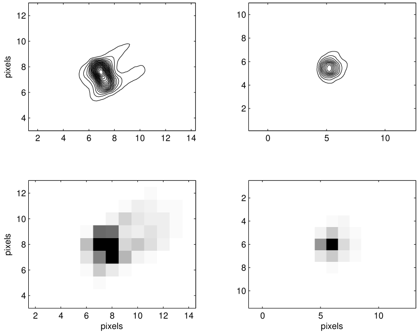
Figure 1: Two example PRFs. Left column: a PRF near the edge of the focal plane. Right column: a PRF near the focal plane center. Top row: the PRF model contours. Bottom row: the PRF converted into pixel values for a star centered on a pixel.

The Kepler PRF on an output channel is represented as a continuous piece-wise polynomial function of sub-pixel position on each pixel, providing a super-resolution image of the light of a star falling on the pixels. Pixel values are determined by evaluating the PRF given the pixel and sub-pixel position of a star: the pixel position determines where the PRF is placed in the output channel’s pixel array, while the sub-pixel position determines the pixel values. Figure 1 shows two example PRFs and corresponding pixel values.

Computation of the PRF from stellar images requires knowing where those images fall on the focal plane. Each star’s coordinates are provided by the Kepler Input Catalog (KIC), and the physical location of the CCDs relative to each other provided by the focal plane geometry (FPG) model (§2.2). Determination of the FPG model, however, requires PRF-fitted stellar centroids (§4.2), so FPG and PRF are mutually dependent. Therefore we determine both FPG and PRF in an iterative process (§3.3).

2.1 Representation of the PRF

A Kepler PRF is defined on a grid of $n\times n$ pixels called the PRF pixel array, where $n$ is large enough to capture the full PRF. Each pixel in the PRF pixel array is sub-divided into $m\times m$ sub-pixel regions. Each sub-pixel region is assigned a two-dimensional polynomial $\mathrm{PRF}_{i,j,s,t}\left(x,y\right)$, where $\left(i,j\right)$ are the pixels indices in the $n\times n$ PRF pixel array and $\left(s,t\right)$ are the sub-pixel indices in the $m\times m$ sub-pixel grid on pixel $\left(i,j\right)$. Therefore there are $n^{2}\times m^{2}$ two-dimensional polynomials associated with a PRF on an output channel. For most channels $n=11$ is sufficient to capture the PRF, while for some channels $n=15$ is required. We find $m=6$ provides sufficient sub-pixel detail. The order of each of these polynomials is determined by a maximal information criterion (§3.2).

Each pixel of the PRF pixel array gives the flux on that pixel from a star whose location is in the central pixel of the PRF pixel array. Thus the central pixel represents the peak of the star’s PRF while pixels towards the edge represent the flux in the wings of that star’s PRF. The values of these fluxes depend on the sub-pixel position of the star.

PRF polynomials are determined independently of each other, so they will not match at sub-pixel boundaries. We handle the resulting discontinuities using two strategies: (1) the discontinuities are minimized by fitting the PRF using data that extends into adjacent sub-pixel regions as described in 3.2 and (2) the remaining discontinuities are smoothed when evaluating the PRF as described in §2.3.

A position-dependent PRF is implemented by measuring five PRFs on each output channel: one at each corner and one at the center. Linear interpolation on the resulting triangles as described in §2.3 provides an interpolated PRF at any point in the output channel. This model neglects pixel-level variations, which are treated during calibration (Jenkins et.al. 2010b, ).

2.2 Focal Plane Geometry

The focal plane geometry (FPG) model represents each of the 42 CCDs on the Kepler focal plane via the center position, rotation angle, and plate scale of each CCD. Prior to launch the CCD positions were known with an accuracy of $\pm 3$ pixels; the FPG model provides the required accuracy of $\pm 0.1$ pixels. The input to the FPG model computation is a two dimensional polynomial which maps right ascension and declination to pixel location. These motion polynomials are derived via a fit to the observed pixel positions of known stars via PRF centroiding (§4.2), and serve as a smoothing filter, reducing the impact of observational errors of individual stars.

FPG computation determines the CCD locations of a set of sky coordinates in two ways: via the raDec2Pix library, which uses the FPG model; and via the motion polynomials, which do not use the FPG model. The FPG model parameters are adjusted via a Levenberg-Marquardt non-linear least squares algorithm until the differences between the model and observation are minimized. The FPG model computation also provides the spacecraft attitude.

2.3 From PRF to Pixel Values

The PRF provides expected pixel values for a given star with a given magnitude and sky location. The output channel and pixel position of the star is determined via the raDec2Pix library. This pixel position determines which triangle contains the star’s central pixel, which determines which three (of five) PRFs are used to compute the star’s final image.

Pixel values for the star are determined from each of the three PRFs by evaluating the PRF polynomials at the sub-pixel position of the star. On each pixel in the PRF pixel array the sub-pixel region containing the star’s sub-pixel coordinates is chosen. The polynomial in that sub-pixel region is evaluated at the star’s sub-pixel location, providing the relative flux for that pixel. This results in an array of $n\times n$ pixels reflecting the relative flux of the star based on that PRF.

When the sub-pixel location of a star is close to the boundary between sub-pixel patches, the following method smoothes out inter-patch discontinuities. The pixel value is evaluated using all nearby polynomial patches (two patches near an edge, four patches near a corner). Adjacent polynomial patches can be evaluated at these positions because patches are defined using data that extend into adjacent patches (§3.2). For simplicity we consider the case of an edge, where we have two values $v_{1}$ and $v_{2}$ from the two polynomial patches adjacent at that edge. These values are smoothly interpolated using the distance $z$ of the star’s sub-pixel position from the edge with the formula $v=w\left(z\right)v_{1}+\left(1-w\left(z\right)\right)v_{2}$. Here the weight $w\left(z\right)$ is given, assuming $z$ is normalized so that it ranges from 0 on one side of the edge to 1 on the other side of the edge, by (Warner, 1983)

$$w\left(z\right)=\frac{f\left(z\right)}{f\left(z\right)+f\left(1-z\right)},\qquad f\left(z\right)=\left\{\begin{array}[]{ll}\exp\left(-1/z^{a}\right)&z>0\\ 0&z\leq 0.\end{array}\right.$$ (1)

The scale factor $a$ determines the steepness of the exponential curve. $w\left(z\right)$ has the property that it is equal to 0 for $z\leq 0$, equal to 1 for $z\geq 1$, and equal to 0.5 for $z=0.5$. Further, $w\left(z\right)$ has continuous derivatives of all order, even at $z=0$ and $z=1$. This approach smoothly eliminates the discontinuity at the boundary between the polynomial patches.

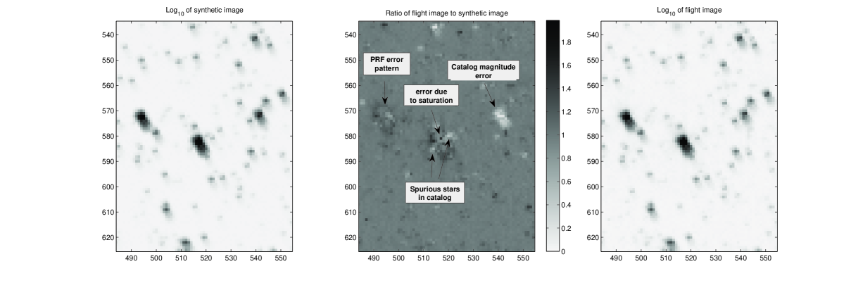
Figure 2: Left: Synthetic image created using a PRF and the Kepler input catalog. Center: Ratio of the the synthetic image and the flight image, indicating various examples of error sources. Right: Flight image for the same region of sky.

The above process is repeated for all three PRFs defined on the triangle containing the star’s central pixel, giving three $n\times n$ pixel arrays, one at the location of each PRF. These pixel arrays are linearly interpolated in the plane of the triangle, giving the final relative pixel values for this star. These relative pixel values are multiplied by the total flux of the star in the Kepler bandpass via the Kepler magnitude given by the Kepler input catalog. The final pixel array is then placed in the output channel pixel array in the location corresponding to the pixel position of the star. Repeating this process for every star on an output channel results in a synthetic image that should match the actual image observed in flight, assuming the KIC is accurate (Figure 2).

3 Measurement of the PRF

The PRF was measured during the commissioning phase of the Kepler mission, after the photometer was brought into final focus. The PRF measurement strategy was to collect observations of bright, uncrowded, unsaturated stars, which are used to fit the PRF polynomial patches.

3.1 In-flight Observations

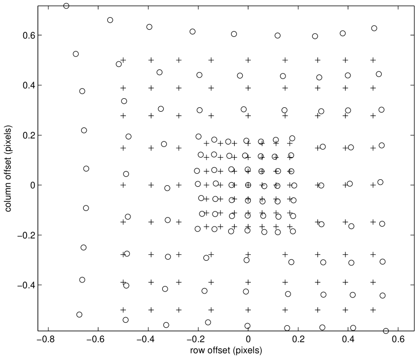
Figure 3: Commanded ($+$) and achieved ($\circ$) dither pattern used to measure the PRF. The discrepancy is due to the early state of calibration of the fine guidance trackers during commissioning.

The PRF measurement used 19,189 stars in the Kepler field with magnitudes between 12 and 13 that did not have significant ($>30\%$) flux from other stars in a $21\times 21$ pixel aperture centered on the star. These stars were observed for 242 cadences of 14.7 minute duration, half a long cadence, to reduce the time required to perform the observations. Data for the PRF measurement were obtained from each odd cadence, while the spacecraft slewed to a new dither location during the even cadences. These 121 PRF data cadences visited the achieved locations shown in Figure 3, which were used in the PRF computation. The order of visitation of this pattern was randomized to minimize the impact of time-varying systematics. The pixel values for each star are converted to relative pixel values by normalizing by the total flux from that star. The pixels from each star measurement of the 121 data cadences are treated as independent data points, resulting in 2,321,869 observations distributed on 84 output channels. The distribution was uneven, with some channels having many more stars than others.

3.2 The PRF Computation

Two types of PRF are computed for each output channel: a single PRF using all targets, and a set of five PRFs to capture intra-channel PRF variation as described in §2.3. When computing the five-PRF set, the data for each of the five PRFs are selected from a region near where that PRF is defined. For each corner PRF the data is selected from a square extending from that corner into the input channel. For the central PRF the data is selected from a square centered on the output channel. The size of each square is set to include a specified minimum number of targets, so the squares on a crowded channel will be smaller than the squares on a channel with fewer stars. We find that ten stars is sufficient to create PRFs that capture the cores with good quality.

Once the data for a particular PRF is selected, the pixel data is grouped in two ways: (1) The integer pixel coordinates of each pixel are registered onto the $n\times n$ PRF pixel array so that the central pixel of the star corresponds to the central pixel of the PRF pixel array. (2) Each star’s pixel is placed into a sub-pixel bin corresponding to the sub-pixel region containing that star. The sub-pixel bin covers a larger area than the sub-pixel region, providing overlapping data used for the polynomial fit, minimizing discontinuities between adjacent polynomial patches. For each pixel in the PRF pixel array, and for each sub-pixel region in that pixel, the $k$th pixel value $p_{k}$ is collected with its sub-pixel coordinates $\left(x_{k},y_{k}\right)$. The PRF polynomial patch $\mathrm{PRF}\left(x_{k},y_{k}\right)$ for that sub-pixel region is the polynomial that minimizes

$$\chi^{2}=\sum_{k=1}^{N}\left[\frac{1}{\sigma_{k}}\left(p_{k}-\mathrm{PRF}\left(x_{k},y_{k}\right)\right)\right]^{2}.$$ (2)

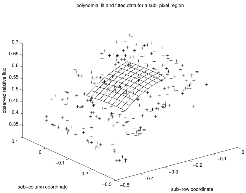
Figure 4: An example of a PRF polynomial patch fitted to data. The domain of the data is larger than the domain of the patch to reduce the size of discontinuities between patches.

Here $N$ is the number of pixel values in this sub-pixel region for this pixel, and $\sigma_{k}$ is the uncertainty in the measurement of $p_{k}$ (Figure 4).

The order of the polynomial is determined by the modified Akaike information criterion (Akaike, 1974). If

$$\mu\left(o\right)=\frac{1}{N}\sum_{k=1}^{N}\left(p_{k}-\mathrm{PRF}_{o}\left(x_{k},y_{k}\right)\right)^{2}.$$ (3)

is the mean square error of the polynomial fit $\mathrm{PRF}_{o}$ for a given order $o$, then Akaike’s modified information criterion selects the order that minimizes

$$2c+N\log\left(\mu\left(o\right)\right)+\frac{2c\left(c-1\right)}{N-c-1}$$ (4)

where $c$ is the number of coefficients in the polynomial $\mathrm{PRF}_{o}$ for order $o$. The polynomial order will vary from sub-pixel region to sub-pixel region. The minimal solution to equation (2) is found using a fitting method that is robust against outliers.

A difficulty was encountered when computing PRFs in a five-PRF set. While the data was sufficient to capture the core of the PRF, the far wings were highly vulnerable to background pollution from dim background stars due to the small number of targets used. In contrast, the single PRFs computed on the same output channel using all the targets had, for the most part, well-behaved wings (we occasionally hand-edited the single PRF far wings to remove obvious background pollution). The solution was to replace polynomials in the far wings of the PRFs in the 5-PRF set with those from the corresponding pixel and sub-pixel regions from the single PRF. The region of replacement was determined by computing a contour of a manually determined background value that encloses the PRF core in each PRF of the five-PRF set. All polynomial patches outside that contour were replaced by polynomials from the single PRF. The resulting discontinuities were of the same magnitude as the discontinuities that already existed between polynomial patches.

The resulting PRFs do a good job of simulating pixel flux from the stars in the KIC, as shown in Figure 2. We find that central pixel energies vary across the Kepler focal plane, with 11% of the output channels having central pixel energies less than 0.3, 20% between 0.3 and 0.4, 37% between 0.4 and 0.5, 28% between 0.5 and 0.6, and 4% between 0.6 and 0.7.

There are several possible sources of PRF error, including:

• Changes in the statistics of spacecraft pointing jitter. This has remained stationary over time but is being monitored.

• Focus has changed slightly but measurably over time due to water desorption and thermal variations (Jenkins et.al. 2010a, ).

• KIC errors, including variable stars and blends, can distort the measured PRF and cause errors for individual stars.

• CCD non-uniformities.

• The PRF computation did not attempt to include effects due to star color. Pre-flight simulated PRFs based on Code V simulations of the optical PSF from Ball Aerospace and Technologies Corporation indicate that color can have a non-trivial effect on the PRF.

The impact and mitigation of these errors is an area of active investigation.

3.3 The FPG/PRF Iteration

The computation described in §3.2 assumes that the pixel data have been calibrated, had their background removed, and that that Kepler attitude and FPG model are known. Pixel data calibration and background removal are performed by the same software from the Kepler SOC pipeline that is used to process Kepler science data (Jenkins et.al. 2010b, ). The Kepler attitude and FPG model, however, are based on PRF centroiding (§4.2). Therefore an iterative approach is required.

Two SOC modules are used: CAL, which performs pixel-level calibration, and PA which performs background characterization and removal as well as stellar centroiding and computation of motion polynomials (PA also performs aperture photometry during Kepler science processing, but PRF does not use this feature). Background-removed pixels are not persisted in the SOC pipeline, so the background removal function of PA must be called with each iteration.

PRF processing begins with a non-iterative bootstrap phase: Pixel data is calibrated by CAL, then PA is called with a pre-launch estimate of the PRF and FPG models that are used for centroiding and motion polynomial creation. At this point the iterative loop is entered: the FPG calculation provides an updated FPG model and attitude solution; PA performs background removal; the PRF computation described in §3.2 is performed; PA performs centroiding and motion polynomial computation using the updated PRF. The iteration is repeated until the FPG model is observed to converge.

To obtain convergence, it was necessary to “pin” the centroid of the PRF computed in §3.2 to a specific location because both PRF and FPG can move the location of a star image on a CCD. We chose to constrain the PRF so that the value-weighted centroid of all input pixel values is at the center of the PRF array.

4 PRF Applications

4.1 Optimal Pixel Selection

There is a limit of $5.4\times 10^{6}$ pixels per Kepler long cadence. Among these pixels are those chosen for stellar Kepler targets (Bathala et.al., 2010). These pixels are selected to support high-precision aperture photometry of these targets: for each stellar target those pixels are selected which maximize the signal-to-noise ratio (SNR) for that target.

The selection process relies on synthetic images generated using the PRF, KIC and a zodiacal light model. For each target, two synthetic images are created: 1) an image that contains the target star only (“target”) and 2) all stars except the target star, plus zodiacal light (“scene”). Both images include effects of saturation, charge transfer efficiency and smear induced by the lack of a shutter. The noise for each pixel $p$ (in electrons) contains contributions from shot, read ($\sigma_{\mathrm{read}}$) and quantization noise ($\sigma_{\mathrm{quant}}$) (Caldwell et.al., 2010) and is computed as $\sigma=\sqrt{p_{\mathrm{target}}+p_{\mathrm{scene}}+\sigma_{\mathrm{read}}^{2}+\sigma_{\mathrm{quant}}^{2}}$. The SNR of the pixel is $p_{\mathrm{target}}/\sigma$.

The pixels are sorted in decreasing order of SNR. Starting with the first pixel, as each pixel is added the SNR of the collection of pixels is computed, and the collection of pixels that maximize the collection’s SNR defines the optimal aperture for this target. Margin against PRF and KIC errors is provided by a ring of pixels placed around the optimal aperture, as well as a column of pixels on the left for undershoot correction (Haas et al., 2010). The result is the requested aperture for storage and downlinking.

Software on the Kepler spacecraft supports 1024 arbitrarily shaped spacecraft apertures, far fewer than the number of requested apertures. Therefore each requested aperture is assigned to the spacecraft aperture with the smallest number of pixels that contains the requested aperture. Figure 5 shows example optimal and spacecraft apertures.

A synthetic image containing all stars in the KIC is used to determine background pixels that are stored, downlinked and used to build and remove a background model in SOC processing of the science targets.

4.2 Stellar Centroids

Centroid locations for unsaturated, sufficiently bright target stars are determined by PRF fitting: a non-linear fit is performed which varies the location and flux of the PRF, minimizing the $\chi^{2}$ of the pixel-wise difference of the PRF-based pixel image (§2.3) and the flight pixel values for that target. The resulting centroids show high stability, with changes over time of about $0.1$ millipixels (after removing systematic effects). Errors in the PRF model induce local biases, which exhibit a median of about 1 millipixel and median absolute deviation of  22 millipixels pixels, across the focal plane.

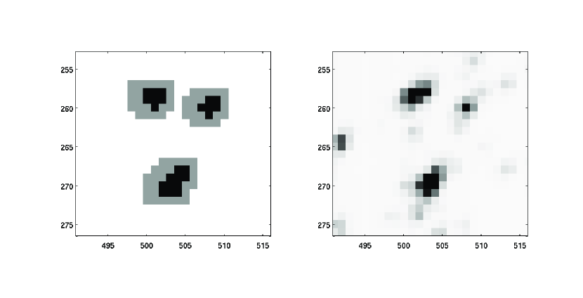
Figure 5: Optimal and spacecraft apertures for three Kepler targets. Left: the optimal apertures for the targets in black and the spacecraft apertures in grey. Right: the synthetic image containing the targets and other stars.

References

- Akaike (1974) Akaike, H., 1974 IEEE Transactions on Automatic Control 19 (6): 716
- Argabright et.al. (2008) Argabright, V. S., et al., 2008 SPIE 7010
- Bathala et.al. (2010) Bathala, N., et al., 2010 ApJ, in press
- Borucki et.al. (2010) Borucki, W. J., et al., 2010 Science, 327 (5968): 977
- Caldwell et.al. (2010) Caldwell, D. A., et al., 2010 ApJ, in press
- Haas et al. (2010) Haas, M. R. et al., 2010 ApJ, in press
- (7) Jenkins, J. M., et al., 2010 ApJ, in press
- (8) Jenkins, J. M., et al., 2010 ApJ, in press
- Koch et.al. (2010) Koch, D. G., et al., 2010 ApJ, in press
- Lauer (1999) Lauer, T. R., 1999 PASP, 111 (765):1434
- Warner (1983) Warner, F. W., 1983, Foundations of Differentiable Manifolds and Lie Groups, (Springer)