Dynamical Horizon Entropy Bound Conjecture in Loop Quantum Cosmology

Abstract

The covariant entropy bound conjecture is an important hint for the quantum gravity, with several versions available in the literature. For cosmology, Ashtekar and Wilson-Ewing ever show the consistence between the loop gravity theory and one version of this conjecture. Recently, S. He and H. Zhang proposed a version for the dynamical horizon of the universe, which validates the entropy bound conjecture for the cosmology filled with perfect fluid in the classical scenario when the universe is far away from the big bang singularity. However, their conjecture breaks down near big bang region. We examine this conjecture in the context of the loop quantum cosmology. With the example of photon gas, this conjecture is protected by the quantum geometry effects as expected.

I Introduction

The thermodynamical property of spacetime is an important hint for the quantization of gravity. Starting from Hawking’s discovery of black hole’s radiation hawking75 , a theory of thermodynamics of spacetime is being constructed gradually. Recently, the second law of this thermodynamics was generalized to the covariant entropy bound conjecture bousso99 . It states that the entropy flux $S$ through any null hypersurface generated by geodesics with non-positive expansion, emanating orthogonally from a two-dimensional (2D) spacelike surface of area $A$, must satisfy

$$\frac{S}{A}\leq\frac{1}{4l_{p}^{2}},$$ (1)

where $l_{p}=\sqrt{\hbar}$ is the Planck length. Here and in what follows, we adopt the units $c=G=k_{B}=1$. Soon, Flanagan, Marolf and Wald flanagan00 proposed a new version of the entropy bound conjecture. If one allows the geodesics generating the null hypersurface from a 2D spacelike surface of area $A$ to terminate at another 2D spacelike surface of area $A^{\prime}$ before coming to a caustic, boundary or singularity of spacetime, one can replace the above conjecture with

$$\frac{S}{A^{\prime}-A}\leq\frac{1}{4l_{p}^{2}}.$$ (2)

More recently, He and Zhang related these conjectures to dynamical horizon and proposed a covariant entropy bound conjecture on the cosmological dynamical horizon zhang07 : Let $A(t)$ be the area of the cosmological dynamical horizon at cosmological time $t$, then the entropy flux $S$ through the cosmological dynamical horizon between time $t$ and $t^{\prime}$ ($t^{\prime}>t$) must satisfy

$$\frac{S}{A(t^{\prime})-A(t)}\leq\frac{1}{4l_{p}^{2}},$$ (3)

if the dominant energy condition holds for matter.

As a non-perturbative and background-independent quantization of gravity, the loop quantum gravity (LQG) developed rapidly in recent years. Its cosmological version, the loop quantum cosmology (LQC) achieved many successes, including resolution of the classical singularity bojowald01 ; bojowald03 , quantum suppression of classical chaotic behavior near singularities bojowald04a ; bojowald04b , generic phase of inflation bojowald02 ; date05 ; xiong1 and more (for example Li ). Since it has been suggested that the holographic principle is a powerful hint and should be used as an essential building block for any quantum gravity theory bousso02 , it is important and tempting to investigate the covariant entropy bound conjecture in the framework of the LQC, which is a successful application of the non-perturbative quantum gravity scheme—the LQG. The authors of ashtekar08 investigated the Bousso’s covariant entropy bound bousso99 ; bousso02 with a cosmology filled with photon gas and found that the conjecture is violated near the big bang in the classical scenario. But they found the LQC can protect this conjecture even in the deep quantum region. In zhang07 , He and Zhang proposed a new version of the entropy bound conjecture for the dynamical horizon in cosmology and validated it through a cosmology filled with adiabatic perfect fluid, governed by the classical Einstein equation when the universe is far away from the big bang singularity. But when the universe approaches the big bang singularity, the strong quantum fluctuation does break down their conjecture. In analogy to Ashtekar and Wilson-Ewing’s result ashtekar08 , one may wonder if He and Zhang’s conjecture can also be protected by the quantum geometry effect of the LQG.

Following ashtekar08 , we use photon gas as an example to investigate this problem. As expected, we find that the loop quantum effects can indeed protect the conjecture. Besides the result of ashtekar08 , our result presents one more evidence for the consistence between the loop gravity and the covariant entropy conjecture. This paper is organized as follows. In Sec. II, we briefly review the framework of the effective LQC and describe the covariant entropy bound conjecture proposed by He and Zhang zhang07 . Then in Sec. III, we test this conjecture with cosmology filled with photon gas, and show that the LQC is able to protect the conjecture in all. We conclude the paper in Sec. IV and discuss the implications.

II The effective framework of LQC and covariant entropy bound conjecture

To a good degree of approximation, the universe can be described by the well-known Friedmann-Robertson-Walker (FRW) metric,

$$ds^{2}=-dt^{2}+a^{2}(t)\left(\frac{dr^{2}}{1-kr^{2}}+r^{2}d\Omega^{2}\right),$$ (4)

which describes a homogeneous and isotropic universe. Here the spatial curvature $k=-1,0,1$ correspond to open, flat and closed universes respectively, and $a$ is the scale factor of the universe. For simplicity we focus on a flat universe in this paper. In the LQC, the phase space for a flat universe is spanned by the coordinates $c=\gamma\dot{a}$, being the gravitational gauge connection, and $p=a^{2}$, being the densitized triad. $\gamma=0.2375$ is the Barbero-Immirzi parameter ashtekar98 . Then the effective Hamiltonian in the LQC is given by ashtekar06 ; mielczarek08

$$H_{eff}=-\frac{3}{8\pi\gamma^{2}\bar{\mu}^{2}}\sqrt{p}\sin^{2}\left(\bar{\mu}c\right)+H_{M}.$$ (5)

The variable $\bar{\mu}$ corresponds to the dimensionless length of the edge of the elementary loop and is given by

$$\bar{\mu}=\xi p^{\lambda},$$ (6)

where $\xi>0$ and $\lambda$ depend on the particular scheme in the holonomy corrections. In this paper we take the $\bar{\mu}$-scheme, which gives

$$\xi^{2}=2\sqrt{3}\pi\gamma l_{p}^{2}$$ (7)

and $\lambda=-1/2$. With this effective Hamiltonian, we have the canonical equation

$$\dot{p}=\left\{p,H_{eff}\right\}=-\frac{8\pi\gamma}{3}\frac{\partial H_{eff}}{\partial c},$$ (8)

or,

$$\dot{a}=\frac{\sin(\bar{\mu}c)\cos(\bar{\mu}c)}{\gamma\bar{\mu}}.$$ (9)

Combining with the constraint on the Hamiltonian, $H_{eff}=0$, we obtain the modified Friedmann equation,

$$H^{2}=\frac{8\pi}{3}\rho\left(1-\frac{\rho}{\rho_{c}}\right),$$ (10)

in terms of the Hubble rate $H\equiv\frac{\dot{a}}{a}$, where $\rho:=\frac{H_{M}}{p^{3/2}}$ and $\rho_{c}=\frac{3}{8\pi\gamma^{2}\bar{\mu}^{2}p}=\frac{\sqrt{3}}{16\pi^{2}\gamma^{2}\hbar}$. $\rho_{c}$ is the critical energy density coming from the quantum effect in the LQC. It is a large quantity and when it goes to infinity all the quantum effects disappear.

According to zhang07 , the cosmological dynamical horizon bousso02 is defined geometrically as a three-dimensional hypersurface foliated by spheres, where at least one orthogonal null congruence with vanishing expansion exists. For a sphere characterized by any value of $(t,r)$, there are two future directed null directions

$$k^{a}_{\pm}=\frac{1}{a}\left(\frac{\partial}{\partial t}\right)^{a}\pm\frac{1}{a^{2}}\left(\frac{\partial}{\partial r}\right)^{a},$$ (11)

satisfying geodesic equation $k^{b}\nabla_{b}k^{a}=0$. The expansion of these null directions is

$$\theta:=\bigtriangledown_{a}k^{a}_{\pm}=\frac{2}{a^{2}}\left(\dot{a}\pm\frac{1}{r}\right),$$ (12)

where the dot denotes differential with respect to $t$, and the sign $+(-)$ represents the null direction pointing to larger (smaller) values of $r$. For an expanding universe, i.e. $\dot{a}>0$, $\theta=0$ determines the location of the dynamical horizon, $r_{H}=1/\dot{a}$, by the definition of dynamical horizon given above. The LQC replaces the big bang with the big bounce, so the universe is symmetric with respect to the point of the bounce, expanding on one side of the bounce and contracting on the other side. The dynamical horizon in the contracting stage of the LQC corresponds to $r_{H}=-1/\dot{a}$, and all of the relations are similar to the ones given here. In this paper we only consider the expanding stage for the LQC, but note that the contracting stage is the same.

Since the area of the dynamical horizon is $A=4\pi a^{2}r_{H}^{2}=4\pi H^{-2}$, the covariant entropy bound conjecture in our question becomes

$$l_{p}^{2}S\leq\pi\left[H^{-2}(t^{\prime})-H^{-2}(t)\right],$$ (13)

where $S$ is the entropy flux through the dynamical horizon between cosmological time $t$ and $t^{\prime}$ ($t^{\prime}>t$), and $H$ is the Hubble parameter. Considering that the cosmology model discussed here is isotropic and homogeneous, we can write the entropy current vector as

$$s^{a}=\frac{s}{a^{3}}\left(\frac{\partial}{\partial t}\right)^{a},$$ (14)

where $s$ is the ordinary comoving entropy density, independent of space. If the entropy current of the perfect fluid is conserved, i.e., $\nabla_{a}s^{a}=0$, $s$ will be independent of $t$ as well. For simplicity we restrict ourselves to this special case. The entropy flux through the dynamical horizon (shown in Fig.1) is given by

$$S=\int_{CDH}s^{a}\epsilon_{abcd}=\frac{4\pi s}{3}\left(r^{3}_{H}(t^{\prime})-r^{3}_{H}(t)\right)$$ (15)

where $\epsilon_{abcd}=a^{3}r^{2}\sin\theta\left(dt\wedge dr\wedge d\theta\wedge d\phi\right)_{abcd}$ is the spacetime volume 4-form. So the conjecture is reduced to

$$H^{-2}(t^{\prime})-\frac{4}{3}l_{p}^{2}s\dot{a}^{-3}(t^{\prime})\geq H^{-2}(t)-\frac{4}{3}l_{p}^{2}s\dot{a}^{-3}(t),~{}~{}t^{\prime}>t.$$

(16)

Figure 1: A schematic of the entropy current flowing across the cosmological dynamical horizon. The thick solid line marked by “CDH” is the cosmological dynamical horizon. The thin solid line is the region enclosed by the CDH at time $t$ and $t^{\prime}$ respectively. The dashed lines are the entropy current.

III Conjecture test for a cosmology filled with perfect fluid

Given that the FRW universe is filled with photon gas, the energy momentum tensor can be expressed as

$$T_{ab} = \rho(t)(dt)_{a}(dt)_{b}+P(t)a^{2}(t)\left\{(dr)_{a}(dr)_{b}\right.$$ (17)

$$\left.+r^{2}[(d\theta)_{a}(d\theta)_{b}+\sin^{2}\theta(d\phi)_{a}(d\phi)_{b}]\right\}.$$

The pressure $P$ and the energy density $\rho$ satisfy a fixed equation of state

$$P=\omega\rho,$$ (18)

where the constant $\omega=\frac{1}{3}$. From $\nabla^{a}T_{ab}=0$, we have the conservation equation

$$\dot{\rho}+3H(\rho+P)=0.$$ (19)

The comoving entropy density $s$ is given by

$$s=a^{3}\frac{\rho+P}{T}=a^{3}(1+\omega)\frac{\rho}{T},$$ (20)

and $\rho$ depends only on the temperature $T$,

$$\rho=K_{o}l_{p}^{-2-\frac{1+\omega}{\omega}}T^{\frac{1+\omega}{\omega}},$$ (21)

where $K_{o}$ is a dimensionless constant depending on the density of energy state of the perfect fluid. For photon gas $K_{o}=\frac{\pi^{2}}{15}$. Plugging above thermodynamics relation into equation (20) we get $s=(1+\omega)K_{o}^{\frac{\omega}{1+\omega}}l_{p}^{-1-\frac{2\omega}{1+\omega}}\rho^{\frac{1}{1+\omega}}a^{3}$. Written the above conservation equation as

$$\dot{\rho}+3(1+\omega)\rho\frac{\dot{a}}{a}=0,$$ (22)

we have an integration constant $C=\rho^{\frac{1}{1+\omega}}a^{3}$. Then $s=(1+\omega)K_{o}^{\frac{\omega}{1+\omega}}l_{p}^{-1-\frac{2\omega}{1+\omega}}C$. Combining our equation of state Eq. (18) with the above conservation equation, we get the relationship between $\rho$ and the Hubble parameter,

$$H=-\frac{1}{3(1+\omega)}\frac{\dot{\rho}}{\rho}.$$ (23)

Substituting the above relation (23) into the modified Friedmann equation (10), we can get

$$\rho=\frac{1}{6\pi(t+C_{1})^{2}(1+\omega)^{2}+\frac{1}{\rho_{c}}}$$ (24)

where $C_{1}$ is an integration constant without direct physical significance, and we can always drop it by resetting the time coordinate. Setting $C_{1}=0$ gives

$$H=\frac{4\pi t\left(1+\omega\right)}{6\pi t^{2}\left(1+\omega\right)^{2}+\frac{1}{\rho_{c}}}.$$ (25)

With the definition of the Hubble parameter, we can integrate once again to get

$$a(t)=C^{1/3}\left[6\pi t^{2}(1+\omega)^{2}+\frac{1}{\rho_{c}}\right]^{\frac{1}{3(1+\omega)}}.$$ (26)

When $\rho_{c}$ goes to infinity, all of the above solutions become the same as the classical ones presented in zhang07 . In the classical scenario,

$$H^{-2}-\frac{4}{3}l_{p}^{2}s\dot{a}^{-3}$$

$$= \frac{9}{4}t^{2}(1+\omega)^{2}-\frac{9K_{o}^{\frac{\omega}{1+\omega}}l_{p}^{1-\frac{2\omega}{1+\omega}}}{2(6\pi)^{1/(1+\omega)}}t^{3-\frac{2}{1+\omega}}(1+\omega)^{4-\frac{2}{1+\omega}}.$$

When $t\ll 1$, $H^{-2}-\frac{4}{3}l_{p}^{2}s\dot{a}^{-3}\sim-t^{3-\frac{2}{1+\omega}}=-t^{3/2}$ which is a decreasing function of $t$, so the conjecture breaks down when the universe approaches the big bang singularity.

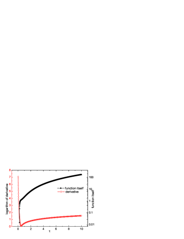
Figure 2: Function $H^{-2}-\frac{4}{3}l_{p}^{2}s\dot{a}^{-3}$ and its derivative respect to $\tau$ for photon gas.

We introduce a new variable $\tau=\sqrt{2\pi\rho_{c}}(1+\omega)t$ for the LQC to simplify the above expressions to

$$H = \sqrt{2\pi\rho_{c}}\frac{2\tau}{3\tau^{2}+1},$$ (28)

$$a = C^{1/3}\rho_{c}^{-\frac{1}{3(1+\omega)}}\left(3\tau^{2}+1\right)^{\frac{1}{3(1+\omega)}},$$ (29)

$$\dot{a}=aH = 2\tau C^{1/3}\rho_{c}^{-\frac{1}{3(1+\omega)}}\sqrt{2\pi\rho_{c}}\left(3\tau^{2}+1\right)^{\frac{1}{3(1+\omega)}-1}.$$

Then

$$H^{-2}-\frac{4}{3}l_{p}^{2}s\dot{a}^{-3}$$

$$= \frac{1}{2\pi\rho_{c}}\left[\left(\frac{3}{2}\tau+\frac{1}{2\tau}\right)^{2}\right.$$

$$- \left.\frac{(1+\omega)}{6\sqrt{2\pi}}K_{o}^{\frac{\omega}{1+\omega}}(\frac{\sqrt{3}}{16\pi^{2}\gamma^{2}})^{\frac{1}{1+\omega}-\frac{1}{2}}\frac{\left(3\tau^{2}+1\right)^{3-\frac{1}{(1+\omega)}}}{\tau^{3}}\right].$$

It is obvious that the necessary and sufficient condition for meeting the covariant entropy bound conjecture is that the above expression increases with $\tau$. In order to investigate the monotone property of above function, we plot $H^{-2}-\frac{4}{3}l_{p}^{2}s\dot{a}^{-3}$ itself and its derivative respect to $\tau$ in Fig.2. The minimal value of the derivative is about $1.16>0$. The covariant entropy bound conjecture for dynamical horizon in cosmology is fully protected by loop quantum effect.

IV conclusion and discussion

The covariant entropy bound conjecture comes from the holographic principle and is an important hint for the quantum gravity theory. In the recent years we have witnessed more and more success of the loop quantum gravity, especially for the problem of the big bang singularity in cosmology. The entropy bound conjecture usually breaks down in the strong gravity region of spacetime where the quantum fluctuation is strong, and one would expect the loop quantum correction to protect the conjecture from the quantum fluctuation. And Ashtekar and Wilson-Ewing do find a result in ashtekar08 which is consistent with above expectation. In this paper, we generalized the covariant entropy conjecture for the cosmological dynamical horizon proposed in zhang07 to the loop quantum cosmology scenario. We found that the quantum geometry effects of the loop quantum gravity can also protect the conjecture. Our result gives out one more evidence for the consistence of covariant entropy conjecture and loop quantum gravity theory. This adds one more encouraging result of loop quantum gravity theory besides previous ones.

- (1) S. W. Hawking, Commun. Math. Phys. 43, 199 (1975).
- (2) R. Bousso, Rev. Mod. Phys. 74, 825 (2002).
- (3) R. Bousso, JHEP 07(1999)004.
- (4) E. Flanagan, D. Marolf and R. Wald, Phys. Rev. D 62, 084035 (2000).
- (5) S. He and H. Zhang, JHEP 10(2007)077.
- (6) M. Bojowald, Phys. Rev. Lett. 86, 5227 (2001).
- (7) M. Bojowald, Class. Quantum Grav. 20, 2595 (2003).
- (8) M. Bojowald, and G. Date, Phys. Rev. Lett. 92, 071302 (2004).
- (9) M. Bojowald, Class. Quantum Grav. 21, 3541 (2004).
- (10) M. Bojowald, Phys. Rev. Lett. 89, 261301 (2002).
- (11) G. Date and G. Hossain, Phys. Rev. Lett. 94, 011301 (2005).
- (12) Hua-Hui Xiong and Jian-Yang Zhu, Phys. Rev. D 75, 084023 (2007).
- (13) Li-Fang Li and Jian-Yang Zhu, Phys. Rev. D 79, 044011 (2009); Phys. Rev. D 79, 124011 (2009); Advances in High Energy Physics, doi:10.1155/2009/905705.
- (14) A. Ashtekar, J. Baez, A. Corichi, and K. Krasnov, Phys. Rev. Lett. 80, 904 (1998).
- (15) A. Ashtekar, T. Pawlowski, and P. Singh, Phys. Rev. D 73, 124038 (2006); 74, 084003 (2006).
- (16) J. Mielczarek, T. Stachowiak, M. Szydlowski, Phys. Rev. D 77, 123506 (2008).
- (17) A. Ashtekar and E. Wilson-Ewing, Phys. Rev. D 78, 064047 (2008).