Regularization for Matrix Completion

Abstract

We consider the problem of reconstructing a low rank matrix from noisy observations of a subset of its entries. This task has applications in statistical learning, computer vision, and signal processing. In these contexts, ‘noise’ generically refers to any contribution to the data that is not captured by the low-rank model. In most applications, the noise level is large compared to the underlying signal and it is important to avoid overfitting. In order to tackle this problem, we define a regularized cost function well suited for spectral reconstruction methods. Within a random noise model, and in the large system limit, we prove that the resulting accuracy undergoes a phase transition depending on the noise level and on the fraction of observed entries. The cost function can be minimized using OptSpace  (a manifold gradient descent algorithm). Numerical simulations show that this approach is competitive with state-of-the-art alternatives.

I Introduction

Let $N$ be an $m\times n$ matrix which is ‘approximately’ low rank, that is

$$N=M+W=U\Sigma V^{T}+W\,.$$ (1)

where $U$ has dimensions $m\times r$, $V$ has dimensions $n\times r$, and $\Sigma$ is a diagonal $r\times r$ matrix. Thus $M$ has rank $r$ and $W$ can be thought of as noise, or ‘unexplained contributions’ to $N$. Throughout the paper we assume the normalization $U^{T}U=m\,I_{r\times r}$ and $V^{T}V=n\,I_{r\times r}$ ($I_{d\times d}$ being the $d\times d$ identity).

Out of the $m\times n$ entries of $N$, a subset $E\subseteq[m]\times[n]$ is observed. We let ${\cal P}_{E}(N)$ be the $m\times n$ matrix that contains the observed entries of $N$, and is filled with $0$’s in the other positions

$${\cal P}_{E}(N)_{ij}=\left\{\begin{array}[]{rl}N_{ij}&\text{if }(i,j)\in E\,,\\ 0&\text{otherwise.}\end{array}\right.$$ (4)

The noisy matrix completion problem requires to reconstruct the low rank matrix $M$ from the observations ${\cal P}_{E}(N)$. In the following we will also write $N^{E}={\cal P}_{E}(N)$ for the sparsified matrix. Over the last year, matrix completion has attracted significant attention because of its relevance –among other applications– to colaborative filtering. In this case, the matrix $N$ contains evaluations of a group of customers on a group of products, and one is interested in exploiting a sparsely filled matrix to provide personalized recommendations [1].

In such applications, the noise $W$ is not a small perturbation and it is crucial to avoid overfitting. For instance, in the limit $M\to 0$, the estimate of $\widehat{M}$ risks to be a low-rank approximation of the noise $W$, which would be grossly incorrect.

In order to overcome this problem, we propose in this paper an algorithm based on minimizing the following cost function

$${\cal F}_{E}(X,Y;S)\equiv\frac{1}{2}||{\cal P}_{E}(N-XSY^{T})||_{F}^{2}+\frac{1}{2}\lambda\,||S||_{F}^{2}\,.$$ (5)

Here the minimization variables are $S\in{\mathds{R}}^{r\times r}$, and $X\in{\mathds{R}}^{m\times r}$, $Y\in{\mathds{R}}^{n\times r}$ with $X^{T}X=Y^{T}Y=I_{r\times r}$. Finally, $\lambda>0$ is a regularization parameter.

I-A Algorithm and main results

The algorithm is an adaptation of the OptSpace  algorithm developed in [2]. A key observation is that the following modified cost function can be minimized by singular value decomposition (see Section I.1):

$$\widehat{\cal F}_{E}(X,Y;S)\equiv\frac{1}{2}||{\cal P}_{E}(N)-XSY^{T}||_{F}^{2}+\frac{1}{2}\lambda\,||S||_{F}^{2}\,.$$ (6)

As emphasized in [2, 3], which analyzed the case $\lambda=0$, this minimization can yield poor results unless the set of observations $E$ is ‘well balanced’. This problem can be bypassed by ‘trimming’ the set $E$, and constructing a balanced set $\widetilde{E}$. The OptSpace  algorithm is given as follows.

OptSpace ( set $E$, matrix $N^{E}$ )
1:	Trim $E$, and let $\widetilde{E}$ be the output;
2:	Minimize $\widehat{\cal F}_{\widetilde{E}}(X,Y;S)$ via SVD,
	let $X_{0},Y_{0},S_{0}$ be the output;
3:	Minimize ${\cal F}_{E}(X,Y;S)$ by gradient descent
	using $X_{0},Y_{0},S_{0}$ as initial condition.

In this paper we will study this algorithm under a model for which step 1 (trimming) is never called, i.e. $\widetilde{E}=E$ with high probability. We will therefore not discuss it any further. Section II compares the behavior of the present approach with alternative schemes. Our main analytical result is a sharp characterization of the mean square error after step 2. Here and below the limit $n\to\infty$ is understood to be taken with $m/n\to\alpha\in(0,\infty)$.

Theorem I.1.

Assume $|M_{ij}|\leq M_{\rm max}$, $W_{ij}$ to be i.i.d. random variables with mean $0$ variance $\sqrt{mn}\sigma^{2}$ and ${\mathbb{E}}\{W_{ij}^{4}\}\leq Cn^{2}$, and that for each entry $(i,j)$, $N_{ij}$ is observed (i.e. $(i,j)\in E$) independently with probability $p$. Finally let $\widehat{M}=X_{0}S_{0}Y_{0}^{T}$ be the rank $r$ matrix reconstructed by step $2$ of OptSpace, for the optimal choice of $\lambda$. Then, almost surely for $n\to\infty$

$$\frac{1}{||M||_{F}^{2}}||\widehat{M}-M||_{F}^{2}=1-$$

$$-\frac{\Big{\{}\sum_{k=1}^{r}\Sigma_{k}^{2}\Big{(}1-\frac{\sigma^{4}}{p^{2}\Sigma^{4}_{k}}\Big{)}_{+}\Big{\}}^{2}}{||\Sigma||_{F}^{2}\Big{\{}\sum_{k=1}^{r}\Sigma_{k}^{2}\Big{(}1+\frac{\sqrt{\alpha}\sigma^{2}}{p\Sigma_{k}^{2}}\Big{)}\Big{(}1+\frac{\sigma^{2}}{p\Sigma_{k}^{2}\sqrt{\alpha}}\Big{)}\Big{\}}}+o_{n}(1)\,.$$

This theorem focuses on a high-noise regime, and predicts a sharp phase transition: if $\sigma^{2}/p<\Sigma_{1}$, we can successfully extract information on $M$, from the observations $N^{E}$. If on the other hand $\sigma^{2}/p\geq\Sigma_{1}$, the observations are essentialy useless in reconstructing $M$. It is possible to prove [4] that the resulting tradeoff between noise and observed entries is tight: no algorithm can obtain relative mean square error smaller than one for $\sigma^{2}/p\geq\Sigma_{1}$, under a simple random model for $M$. To the best of our knowledge, this is the first sharp phase transition result for low rank matrix completion.

For the proof of Theorem I.1, we refer to Section III. An important byproduct of the proof is that it provides a rule for choosing the regularization parameter $\lambda$, in the large system limit.

I-B Related work

The importance of regularization in matrix completion is well known to practitioners. For instance, one important component of many algorithms competing for the Netflix challenge [1], consisted in minimizing the cost function ${\cal H}_{E}(X,Y;S)\equiv\frac{1}{2}||{\cal P}_{E}(N-\widetilde{X}\widetilde{Y}^{T})||_{F}^{2}+\frac{1}{2}\lambda\,||\widetilde{X}||_{F}^{2}+\frac{1}{2}\lambda\,||\widetilde{Y}||_{F}^{2}$ (this is also known as maximum margin matrix factorization [5, 6]). Here the minimization variables are $\widetilde{X}\in{\mathds{R}}^{m\times r}$, $\widetilde{Y}\in{\mathds{R}}^{n\times r}$. Unlike in OptSpace, these matrices are not constrained to be orthogonal, and as a consequence the problem becomes significantly more degenerate. Notice that, in our approach, the orthogonality constraint fixes the norms $||X||_{F}$, $||Y||_{F}$. This motivates the use of $||S||_{F}^{2}$ as a regularization term.

Convex relaxations of the matrix completion problem were recently studied in [7, 8]. As emphasized by Mazumder, Hastie and Tibshirani [9], such nuclear norms relaxations can be viewed as spectral regularizations of a least square problem. Finally, the phase transition phenomenon in Theorem I.1, generalizes a result of Johnstone and Lu on principal component analysis [10], and similar random matrix models were studied in [11].

II Numerical simulations

In this section, we present the results of numerical simulations on synthetically generated matrices. The data are generated following the recipe of [9]: sample ${\overline{U}}\in{\mathds{R}}^{n\times r}$ and ${\overline{V}}\in{\mathds{R}}^{m\times r}$ by choosing ${\overline{U}}_{ij}$ and ${\overline{V}}_{ij}$ independently and indentically as ${\cal N}(0,1)$. Sample independently $W\in{\mathds{R}}^{m\times n}$ by choosing $W_{ij}$ iid with distribution ${\cal N}(0,\sigma^{2}\sqrt{mn})$. Set $N={\overline{U}}{\overline{V}}^{T}+W$. We also use the parameters chosen in [9] and define

$${\rm SNR} = \sqrt{\frac{{\rm Var}(({\overline{U}}{\overline{V}}^{T})_{ij})}{{\rm Var}(W_{ij})}}\,,$$

$${\rm TestError} = \frac{||{\cal P}_{E}^{\perp}({\overline{U}}{\overline{V}}^{T}-\widehat{N})||_{F}^{2}}{||{\cal P}_{E}^{\perp}(UV^{T})||_{F}^{2}}\,,$$

$${\rm TrainError} = \frac{||{\cal P}_{E}(N-\widehat{N})||_{F}^{2}}{||{\cal P}_{E}(N)||_{F}^{2}}\,,$$

where ${\cal P}_{E}^{\perp}(A)\equiv A-{\cal P}_{E}(A)$.

In Figure 1, we plot the train error and test error for the OptSpace algorithm on matrices generated as above with $n=100,r=10$, SNR=$1$ and $p=0.5$. For comparison, we also plot the corresponding curves for Soft-Impute,Hard-Impute and SVT taken from [9]. In Figures 2 and 3, we plot the same curves for different values of $r,\epsilon,{\rm SNR}$. In these plots, OptSpace$(\lambda)$ corresponds to the algorithm that minimizes the cost (5). In particular OptSpace$(0)$ corresponds to the algorithm described in [2]. Further, $\lambda^{*}=\lambda^{*}(\rho)$ is the value of the regularization parameter that minimizes the test error while using rank $\rho$ (this can be estimated on a subset of the data, not used for training).

It is clear that regularization greatly improves the performance of OptSpace  and makes it competitive with the best alternative methods.

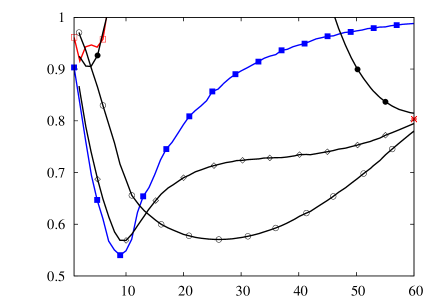
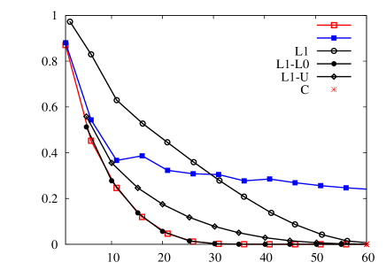
Figure 1: Test (top) and train (bottom) error vs. rank for OptSpace, Soft-Impute, Hard-Impute and SVT. Here $m=n=100,r=10,p=0.5,{\rm SNR}=1$.

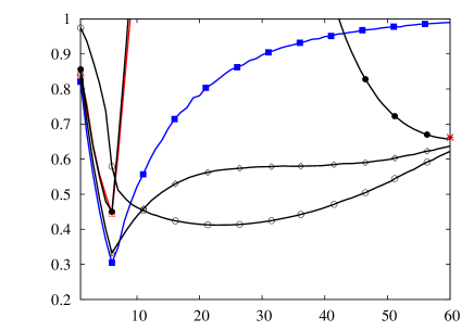
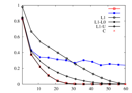
Figure 2: Test (top) and train (bottom) error vs. rank for OptSpace, Soft-Impute, Hard-Impute and SVT. Here $m=n=100,r=6,p=0.5,{\rm SNR}=1$.

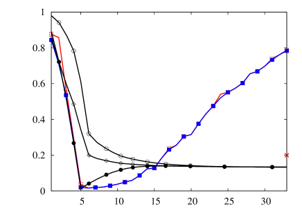
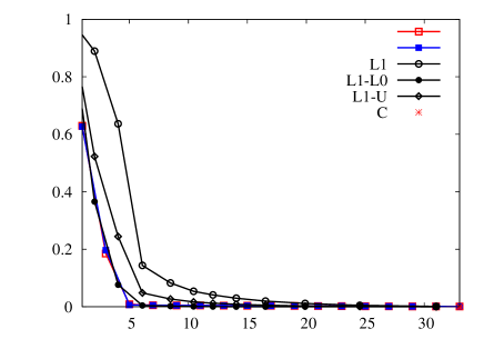
Figure 3: Test (top) and train (bottom) error vs. rank for OptSpace, Soft-Impute, Hard-Impute and SVT. Here $m=n=100,r=5,p=0.2,{\rm SNR}=10$.

III Proof of Theorem I.1

The proof of Theorem 1 is based on the following three steps: $(i)$ Obtain an explicit expression for the root mean square error in terms of right and left singular vectors of $N$; $(ii)$ Estimate the effect of the noise $W$ on the right and left singular vectors; $(iii)$ Estimate the effect of missing entries. Step $(ii)$ builds on recent estimates on the eigenvectors of large covariance matrices [12]. In step $(iii)$ we use the results of [2]. Step $(i)$ is based on the following linear algebra calculation, whose proof we omit due to space constraints (here and below $\langle A,B\rangle\equiv{\rm Tr}(AB^{T})$).

Proposition III.1.

Let $X_{0}\in{\mathds{R}}^{m\times r}$ and $Y_{0}\in{\mathds{R}}^{m\times r}$ be the matrices whose columns are the first $r$, right and left, singular vectors of $N^{E}$. Then the rank-$r$ matrix reconstructed by step $2$ of of OptSpace, with regularization parameter $\lambda$, has the form $\widehat{M}(\lambda)=X_{0}S_{0}(\lambda)Y_{0}^{T}$ Further, there exists $\lambda_{*}>0$ such that

$$\frac{1}{mn}||M-\widehat{M}(\lambda_{*})||_{F}^{2}=||\Sigma||_{F}^{2}-\left(\frac{\langle X_{0}^{T}MY_{0}\,,\,X_{0}^{T}N^{E}Y_{0}\rangle}{\sqrt{mn}||X_{0}N^{E}Y_{0}||_{F}}\right)^{2}\,.$$ (7)

III-A The effect of noise

In order to isolate the effect of noise, we consider the matrix $\widehat{N}=p\,U\Sigma V^{T}+W^{E}$. Throughout this section we assume that the hypotheses of Theorem I.1 hold.

Lemma III.2.

Let $(nz_{1,n},\dots,nz_{r,n})$ be the $r$ largest singular values of $\widehat{N}$. Then, as $n\to\infty$, $z_{i,n}\to z_{i}$ almost surely, where, for $\Sigma_{i}^{2}>\sigma^{2}/p$,

$$z_{i}=p\Sigma_{i}\left\{\alpha\left(\frac{\sigma^{2}}{p\Sigma_{i}^{2}}+\frac{1}{\sqrt{\alpha}}\right)\left(\frac{\sigma^{2}}{p\Sigma_{i}^{2}}+\sqrt{\alpha}\right)\right\}^{1/2}\,,$$ (8)

and $z_{i}=\sigma\sqrt{p\alpha^{1/2}}(1+\sqrt{\alpha})$ for $\Sigma_{i}^{2}\leq\sigma^{2}/p$.

Further, let $X\in{\mathds{R}}^{m\times r}$ and $Y\in{\mathds{R}}^{n\times r}$ be the matrices whose columns are the first $r$, right and left, singular vectors of $\widehat{N}$. Then there exists a sequence of $r\times r$ orthogonal matrices $Q_{n}$ such that, almost surely $||\frac{1}{\sqrt{m}}U^{T}X-AQ_{n}||_{F}\to 0$, $||\frac{1}{\sqrt{n}}V^{T}Y-BQ_{n}||_{F}\to 0$ with $A={\rm diag}(a_{1},\dots,a_{r})$, $B={\rm diag}(b_{1},\dots,b_{r})$ and

$$a_{i}^{2} = \Big{(}1-\frac{\sigma^{4}}{p^{2}\Sigma_{i}^{4}}\Big{)}\Big{(}1+\frac{\sqrt{\alpha}\sigma^{2}}{p\Sigma_{i}^{2}}\Big{)}^{-1}\,,$$

$$b_{i}^{2} = \Big{(}1-\frac{\sigma^{4}}{p^{2}\Sigma_{i}^{4}}\Big{)}\Big{(}1+\frac{\sigma^{2}}{p\sqrt{\alpha}\Sigma_{i}^{2}}\Big{)}^{-1}\,,$$ (9)

for $\Sigma_{i}^{2}>\sigma^{2}/p$, while $a_{i}=b_{i}=0$ otherwise.

Proof:

Due to space limitations, we will focus here on the case $\Sigma_{1},\dots,\Sigma_{r}>\sigma^{2}/p$. The general proof proceeds along the same lines, and we defer it to [4].

Notice that $W^{E}$ is an $m\times n$ matrix with i.i.d. entries with variance $\sqrt{mn}\sigma^{2}p$ and fourth moment bounded by $Cn^{2}$. It is therefore sufficient to prove our claim for $p=1$ and then rescale $\Sigma$ by $p$ and $\sigma$ by $\sqrt{p}$. We will also assume that, without loss of generality, $m\geq n$.

Let $\widehat{Z}$ be an $r\times r$ diagonal matrix containing the eigenvalues $(nz_{n,1},\dots,nz_{n,r})$. The eigenvalue equations read

$$U\hat{\beta}_{y}+WY-X\widehat{Z} = 0\,,$$ (10)

$$V\hat{\beta}_{x}+W^{T}X-Y\widehat{Z} = 0\,.$$ (11)

where we defined $\hat{\beta}_{x}\equiv\Sigma\,U^{T}X$, $\hat{\beta}_{y}\equiv\Sigma\,V^{T}Y\in{\mathds{R}}^{r\times r}$. By singular value decomposition we can write $W=L\,{\rm diag}(w_{1},w_{2},\ldots w_{n})R^{T}$, with $L^{T}L=I_{m\times m}$, $R^{T}R=I_{n\times n}$.

Let $u_{i}^{T}$, $x_{i}^{T}$, $v_{i}^{T}$, $y_{i}^{T}\in{\mathds{R}}^{r}$ be the $i$-th row of -respectively- $L^{T}U$, $L^{T}X$, $R^{T}V$, $R^{T}Y$. In this basis equations (10) and (11) read

$$u_{i}^{T}\hat{\beta}_{y}+w_{i}y_{i}^{T}-x_{i}^{T}\widehat{Z} = 0\,,\qquad i\in[n]\,,$$

$$u_{i}^{T}\hat{\beta}_{y}-x_{i}^{T}\widehat{Z} = 0\,,\qquad i\in[m]\backslash[n]\,,$$

$$v_{i}^{T}\hat{\beta}_{x}+w_{i}x_{i}^{T}-y_{i}^{T}\widehat{Z} = 0\,,\qquad i\in[n]\,.$$

These can be solved to get

$$x_{i}^{T} = (u_{i}^{T}\hat{\beta}_{y}\widehat{Z}+w_{i}v_{i}^{T}\hat{\beta}_{x})(Z^{2}-w_{i}^{2})^{-1}\,,\qquad i\in[n]\,,$$

$$x_{i}^{T} = u_{i}^{T}\hat{\beta}_{y}\widehat{Z}^{-1}\,,\qquad\qquad\qquad\qquad\qquad\;\;\;\;\;\;i\in[m]\backslash[n]\,,$$

$$y_{i}^{T} = (v_{i}^{T}\hat{\beta}_{x}\widehat{Z}+w_{i}u_{i}^{T}\hat{\beta}_{y})(\widehat{Z}^{2}-w_{i}^{2})^{-1}\,,\qquad i\in[n].$$ (12)

By definition $\Sigma^{-1}\hat{\beta}_{x}=\sum_{i=1}^{m}u_{i}x_{i}^{T}$, and $\Sigma^{-1}\hat{\beta}_{y}=\sum_{i=1}^{n}v_{i}y_{i}^{T}$, whence

$$\Sigma^{-1}\hat{\beta}_{x} = \sum_{i=1}^{n}u_{i}(u_{i}^{T}\hat{\beta}_{y}\widehat{Z}+w_{i}v_{i}^{T}\hat{\beta}_{x})(\widehat{Z}^{2}-w_{i}^{2})^{-1}$$ (13)

$$+\sum_{i=n+1}^{m}u_{i}u_{i}^{T}\beta_{y}\widehat{Z}^{-1}\,,$$

$$\Sigma^{-1}\hat{\beta}_{y} = \sum_{i=1}^{n}v_{i}(v_{i}^{T}\hat{\beta}_{x}\widehat{Z}+w_{i}u_{i}^{T}\hat{\beta}_{y})(\widehat{Z}^{2}-w_{i}^{2})^{-1}.$$ (14)

Let $\lambda=w_{i}^{2}\alpha^{1/2}/(m^{2}\sigma^{2})$. Then, it is a well known fact [13] that as $n\to\infty$ the empirical law of the $\lambda_{i}$’s converges weakly almost surely to the Marcenko-Pastur law, with density $\rho(\lambda)=\alpha\sqrt{(\lambda-c_{-}^{2})(c_{+}^{2}-\lambda)}/(2\pi\lambda)$, with $c_{\pm}=1\pm\alpha^{-1/2}$.

Let $\beta_{x}=\hat{\beta}_{x}/\sqrt{m}$, $\beta_{y}=\hat{\beta}_{x}/\sqrt{n}$, $Z=\widehat{Z}/n$. A priori, it is not clear that the sequence $(\beta_{x},\beta_{y},Z)$ –dependent on $n$– converges. However, it is immediate to show that the sequence is tight, and hence we can restrict ourselves to a subsequence $\Xi\equiv\{n_{i}\}_{i\in{\mathds{N}}}$ along which a limit exists. Eventually we will show that the limit does not depend on the subsequence, apart, possibly, from the rotation $Q_{n}$. Hence we shall denote the subsequential limit, by an abuse of notation, as $(\beta_{x},\beta_{y},Z)$.

Consider now a such a convergent subsequence. It is possible to show that $\Sigma_{i}^{2}>\sigma^{2}/p$ implies $Z_{ii}^{2}>\alpha^{3/2}\sigma^{2}c_{+}(\alpha)^{2}+\delta$ for some positive $\delta$. Since almost surely as $n\to\infty$, $w_{i}^{2}<\alpha^{3/2}\sigma^{2}c_{+}(\alpha)^{2}+\delta/2$ for all $i$, for all purposes the summands on the rhs of Eqs. (13), (14) can be replaced by uniformly continuous, bounded functions of the limiting eigenvalues $\lambda_{i}$. Further, each entry of $u_{i}$ (resp. $v_{i}$) is just a single coordinate of the left (right) singular vectors of the random matrix $W$. Using Theorem $1$ in [12], it follows that any subsequential limit satisfies the equations

$$\beta_{x} =\Sigma\beta_{y}\Big{\{}Z\int(Z^{2}-\alpha^{3/2}\sigma^{2}\lambda)^{-1}\rho(\lambda){\rm d}\lambda+(\alpha-1)Z^{-1}\Big{\}}\,,$$ (15)

$$\beta_{y} =\Sigma\beta_{x}\Big{\{}Z\int(Z^{2}-\alpha^{3/2}\sigma^{2}\lambda)^{-1}\,\rho(\lambda)\,{\rm d}\lambda\Big{\}},.$$ (16)

Solving for $\beta_{y}$, we get an equation of the form

$$\Sigma^{-2}\beta_{y}=\beta_{y}\,f(Z)$$ (17)

where $f(\,\cdot\,)$ is a function that can be given explicitely using the Stieltjis transform of the measure $\rho(\lambda){\rm d}\lambda$. Equation (17) implies that $\beta_{y}$ is block diagonal according to the degeneracy pattern of $\Sigma$. Considering each block, either $\beta_{y}$ vanishes in the block (a case that can be excluded using $\Sigma_{i}^{2}>\sigma^{2}/p$) or $\Sigma_{i}^{-2}=f(Z_{ii})$ in the block. Solving for $Z_{ii}$ shows that the eigenvalues are uniquely determined (independent of the subsequence) and given by Eq. (8).

In order to determine $\beta_{x}$ and $\beta_{y}$ first observe that, since $I_{r\times r}=Y^{T}Y=\sum_{i=1}^{n}y_{i}y_{i}^{T}$, we have, using Eq. (12)

$$I_{r\times r} = \sum_{i=1}^{n}(\widehat{Z}^{2}-w_{i}^{2})^{-1}(\widehat{Z}\hat{\beta}_{x}^{T}v_{i}+w_{i}\hat{\beta}_{y}^{T}u_{i})$$

$$(v_{i}^{T}\hat{\beta}_{x}\widehat{Z}+w_{i}u_{i}^{T}\hat{\beta}_{y})(\widehat{Z}^{2}-w_{i}^{2})^{-1}\,.$$

In the limit $n\to\infty$, and assuming a convergent subsequence for $(Z,\beta_{x},\beta_{y})$, this sum can be computed as above. After

$$I_{r\times r} = \Big{\{}\int\frac{Z^{2}}{(Z^{2}-\alpha^{3/2}\sigma^{2}\lambda)^{2}}\rho(\lambda)\,{\rm d}\lambda\Big{\}}C_{x}$$

$$+\Big{\{}\int\frac{\alpha^{3/2}\sigma^{2}\lambda}{(Z^{2}-\alpha^{3/2}\sigma^{2}\lambda)^{2}}\rho(\lambda)\,{\rm d}\lambda\Big{\}}C_{y}\,,$$

where $C_{x}=\beta_{x}^{T}\beta_{x}$, $C_{y}=\beta_{y}^{T}\beta_{y}$ and the functions of $Z$ on the rhs are defined as standard analyic functions of matrices.

Using Eqs. (15), (16) and solving the above, we get $C_{x}={\rm diag}(\Sigma_{1}^{2}a_{1}^{2},\dots\Sigma_{r}^{2}a_{r}^{2})$, and $B_{y}={\rm diag}(\Sigma_{1}^{2}b_{1}^{2},\dots\Sigma_{r}^{2}b_{r}^{2})$. We already concluded that $\beta_{x}$ and $\beta_{y}$ are block diagonals with blocks in correspondence with the degeneracy pattern of $\Sigma$. Since $\beta_{x}^{T}\beta_{x}=C_{x}$ and $\beta_{y}^{T}\beta_{y}=C_{y}$ are diagonal, with the same degeneracy pattern, it follows that, inside each block of size $d$, each of $\beta_{x}$ and $\beta_{y}$ is proportional to a $d\times d$ orthogonal matrix. Therefore $\beta_{x}=\Sigma AQ_{s}$, $\beta_{y}=\Sigma BQ^{\prime}_{s}$, for some othogonal matriced $Q_{s}$, $Q_{s}^{\prime}$. Also, using equation (15) one can prove that $Q_{s}=Q_{s}^{\prime}$.

Notice, by the above argument $A$, $B$ are uniquely fixed by our construction. On the other hand $Q_{s}$ might depend on the subsequence $\Xi$. Since our statmement allows for a seqence of rotations $Q_{n}$, that depend on $n$, the eventual subsequence dependence of $Q_{s}$ can be factored out. ∎

It is useful to point out a straightforward consequence of the above.

Corollary III.3.

There exists a sequence of orthogonal matrices $Q_{n}\in{\mathds{R}}^{r\times r}$ such that, almost surely,

$$\lim_{n\to\infty}\Big{|}\Big{|}\frac{1}{\sqrt{mn}}X^{T}U\Sigma V^{T}Y-Q_{n}DQ^{T}_{n}\Big{|}\Big{|}_{F} = 0\,,$$ (18)

with $D={\rm diag}(\Sigma_{1}a_{1}b_{1},\dots,\Sigma_{r}a_{r}b_{r})$.

III-B The effect of missing entries

The proof of Theorem I.1 is completed by estabilishing a relation between the singular vectors $X_{0}$, $Y_{0}$ of $N^{E}$ and the singular vectors $X$ and $Y$ of $\widehat{N}$.

Lemma III.4.

Let $k\leq r$ be the largest integer such that $\Sigma_{1}\geq\dots\geq\Sigma_{k}>\sigma^{2}/p$, and denote by $X_{0}^{(k)}$, $Y_{0}^{(k)}$, $X^{(k)}$, and $Y^{(k)}$ the matrices containing the first $k$ columns of $X_{0}$, $Y_{0}$, $X$, and $Y$, respectively. Let $X^{(k)}_{0}=X^{(k)}S_{x}+X^{(k)}_{\perp}$, $Y^{(k)}_{0}=Y^{(k)}S_{y}+Y^{(k)}_{\perp}$ where $(X^{(k)}_{\perp})^{T}X^{(k)}=0$, $(Y^{(k)}_{\perp})^{T}Y^{(k)}=0$ and $S_{x},S_{y}\in{\mathds{R}}^{r\times r}$. Then there exists a numerical constant $C=C(\Sigma_{i},\sigma^{2},\alpha,M_{\rm max})$, such that, with high probability,

$$||X_{\perp}^{(k)}||_{F}^{2},||Y_{\perp}^{(k)}||_{F}^{2}\leq Cr\,\sqrt{\frac{1}{n}}\,,$$ (19)

with probability approaching $1$ as $n\to\infty$.

Proof:

We will prove our claim for the right singular vector $Y$, since the left case is completely analogous. Further we will drop the superscript $k$ to lighten the notation.

We start by noticing that $||N^{E}Y_{0}||_{F}^{2}=\sum_{a=1}^{k}(n\tilde{z}_{a,n})^{2}$, where $n\tilde{z}_{a,n}$ are the singular values of $N^{E}$. Using Lemma 3.2 in [2] which bounds $||M^{E}-pM||_{2}=||N^{E}-\widehat{N}||_{2}$, we get

$$||N^{E}Y_{0}||_{F}^{2} \geq \sum_{a=1}^{k}\left(nz_{a,n}-CM_{\rm max}\sqrt{pn}\right)^{2}\,.$$ (20)

On the other hand $||N^{E}Y_{0}||_{F}\leq||\widehat{N}Y_{0}||_{F}+||N^{E}-\widehat{N}||_{2}||Y_{0}||_{F}$. Further by letting $S_{y}=L_{y}\Theta_{y}R_{y}^{T}$, for $L_{y},R_{y}$ orthogonal matrices, we get $||\widehat{N}Y_{0}||_{F}^{2}=||\widehat{N}YL_{y}\Theta_{y}||_{F}^{2}+||\widehat{N}Y_{\perp}||_{F}^{2}$. Since $Y_{0}^{T}Y_{0}=I_{k\times k}$, we have $I_{k\times k}=R_{y}\Theta_{y}^{T}\Theta_{y}R_{y}^{T}+Y_{\perp}^{T}Y_{\perp}$, and therefore

$$||\widehat{N}Y_{0}||_{F}^{2} = ||\widehat{N}YL_{y}||_{F}^{2}-||\widehat{N}YL_{y}R_{y}^{T}Y_{\perp}^{T}||_{F}^{2}+||\widehat{N}Y_{\perp}||_{F}^{2}$$

$$\leq n^{2}\sum_{a=1}^{k}z_{a,n}^{2}-n^{2}z_{k,n}^{2}||Y_{\perp}||_{F}^{2}$$

$$+n^{2}p\sigma^{2}\alpha(c_{+}(\alpha)+\delta)||Y_{\perp}||_{F}^{2}$$

$$= n^{2}\sum_{a=1}^{k}z_{a,n}^{2}-n^{2}e_{y}||Y_{\perp}||_{F}^{2}\,,$$

where $e_{y}\equiv z_{k,n}^{2}-p\sigma^{2}\alpha(c_{+}(\alpha)+\delta)$, and used the inequality $||\widehat{N}Y_{\perp}||_{F}^{2}\leq n^{2}p\sigma^{2}\alpha(c_{+}(\alpha)+\delta)||Y_{\perp}||_{F}^{2}$ which holds for all $\delta>0$ asymptotically almost surely as $n\to\infty$ (by an immediate generalization of Lemma III.2). It is simple to check that $\Sigma_{k}\geq\sigma^{2}/p$ implies $e_{y}>0$.

Using triangular inequality, Lemma 3.2 in [2], we get

$$||NY_{0}||_{F}^{2} \leq n^{2}\sum_{a=1}^{r}z_{a,n}^{2}-n^{2}e_{y}||Y_{\perp}||_{F}^{2}+Cnp\alpha^{3/2}M_{\rm max}^{2}r$$

$$+2Cn\sqrt{np}\alpha^{3/4}M_{\rm max}\sqrt{r}||z||\,,$$

which, combined with equation (20), implies the thesis. ∎

Proof:

We now turn to upper bounding the right hand side of Eq. (7). Let $k$ be defined as in the last lemma. Notice that by Lemma III.2, $X^{T}(U\Sigma V^{T})Y$ is well approximated by $(X^{(k)})^{T}(U\Sigma V^{T})Y^{(k)}$. Analogously, it can be proved that $X^{T}_{0}(U\Sigma V^{T})Y_{0}$ is well approximated by $(X^{(k)}_{0})^{T}(U\Sigma V^{T})Y^{(k)}_{0}$. Due to space limitations, we will omit this technical step and thus focus here on the case $k=r$ (equivalently, neglect the error incurred by this approximation).

Using Lemma III.4 to bound the contribution of $X_{\perp},Y_{\perp}$, we have

$$\langle X_{0}^{T}(U\Sigma V^{T})Y_{0}\,,\,X_{0}^{T}N^{E}Y_{0}\rangle$$

$$=\langle S_{x}^{T}X^{T}(U\Sigma V^{T})YS_{y}\,,\,X_{0}^{T}N^{E}Y_{0}\rangle(1+o_{n}(1))$$

$$=\langle X^{T}(U\Sigma V^{T})Y\,,\,S_{x}^{T}X_{0}^{T}N^{E}Y_{0}S_{y}\rangle(1+o_{n}(1))\,.$$ (21)

Further $X_{0}^{T}N^{E}Y_{0}=X_{0}^{T}\widehat{N}Y_{0}+X_{0}^{T}(N^{E}-\widehat{N})Y_{0}$ and, using once more the bound in Lemma 3.2 of [2], that implies $|X_{0}^{T}(N^{E}-\widehat{N})Y_{0}|\leq Cr\sqrt{nrp}$, we get

$$S_{x}^{T}X_{0}^{T}N^{E}Y_{0}S_{y} = L_{x}\Theta_{x}^{2}L_{x}^{T}X^{T}\widehat{N}YR_{y}\Theta_{y}^{2}R^{T}_{y}+E_{1}$$

$$= Z+E_{2}\,,$$

where we recall that $Z$ is the diagonal matrix with entries given by the singular values of $\widehat{N}$, and $||E_{1}||_{F}^{2},||E_{2}||_{F}^{2}\leq C(p,r)\sqrt{n}$. Using this estimate in Eq. (21), together with the result in Lemma III.2, we finally get

$$\frac{\langle X_{0}^{T}(U\Sigma V^{T})Y_{0}\,,\,X_{0}^{T}N^{E}Y_{0}\rangle}{\sqrt{mn}||X_{0}^{T}N^{E}Y_{0}||_{F}^{2}}\geq\frac{\sum_{k=1}^{r}\Sigma_{k}a_{k}b_{k}z_{k}}{\sqrt{\alpha}||z||}-o_{n}(1)\,,$$

which implies the thesis after simple algebraic manipulations ∎

References

- [1] “Netflix prize,” http://www.netflixprize.com/.
- [2] R. H. Keshavan, A. Montanari, and S. Oh, “Matrix completion from a few entries,” January 2009, arxiv:0901.3150.
- [3] ——, “Matrix completion from noisy entries,” June 2009, arXiv:0906.2027.
- [4] R. H. Keshavan and A. Montanari, “Regularization for matrix completion,” 2010, journal version, in preparation.
- [5] N. Srebro, J. Rennie, and T. Jaakkola, “Maximum margin matrix factorization,” in Advances in Neural Information Processing Systems 17, 2005.
- [6] J. Rennie and N. Srebro, “Fast maximum margin matrix factorization for collaborative prediction,” in 22nd International Conference on Machine Learning, 2005.
- [7] E. J. Candès and B. Recht, “Exact matrix completion via convex optimization,” Found. of Comput. Math., vol. 9, no. 6, pp. 717 – 772, 2009.
- [8] E. J. Candès and Y. Plan, “Matrix completion with noise,” 2009, arXiv:0903.3131.
- [9] R. Mazumder, T. Hastie, and R. Tibshirani, “Spectral regularization algorithms for learning large incomplete matrices,” 2009, submitted.
- [10] I. M. Johnstone and A. Y. Lu, “On consistency and sparsity for principal component analysis in high dimension,” J. Amer. Stat. Assoc., vol. 104, pp. 682–693, 2009.
- [11] M. Capitaine, C. Donati-Martin, and D. Féral, “The largest eigenvalue of finite rank deformation of large wigner matrices: convergence and non-universality of the fluctuations,” Ann. Probab., vol. 37, pp. 1–47, 2009.
- [12] Z.D.Bai, B.Q.Miao, and G.M.Pan, “On asymptotics of eigenvectors of large sample covariance matrices,” Ann. of Probab., vol. 35, pp. 1532–1572, 2007.
- [13] J. Silverstein and Z. Bai, “On the empirical distribution of eigenvalues of a class of large-dimentional random matrices,” J. Multivariate Anal., vol. 54, pp. 175–192, 1995.