Realization of the Exactly Solvable Kitaev Honeycomb Lattice Model in a Spin Rotation Invariant System

Abstract

The exactly solvable Kitaev honeycomb lattice model is realized as the low energy effect Hamiltonian of a spin-1/2 model with spin rotation and time-reversal symmetry. The mapping to low energy effective Hamiltonian is exact, without truncation errors in traditional perturbation series expansions. This model consists of a honeycomb lattice of clusters of four spin-1/2 moments, and contains short-range interactions up to six-spin(or eight-spin) terms. The spin in the Kitaev model is represented not as these spin-1/2 moments, but as pseudo-spin of the two-dimensional spin singlet sector of the four antiferromagnetically coupled spin-1/2 moments within each cluster. Spin correlations in the Kitaev model are mapped to dimer correlations or spin-chirality correlations in this model. This exact construction is quite general and can be used to make other interesting spin-1/2 models from spin rotation invariant Hamiltonians. We discuss two possible routes to generate the high order spin interactions from more natural couplings, which involves perturbative expansions thus breaks the exact mapping, although in a controlled manner.

I Introduction.

Kitaev’s exactly solvable spin-1/2 honeycomb lattice modelKitaev (noted as the Kitaev model hereafter) has inspired great interest since its debut, due to its exact solvability, fractionalized excitations, and the potential to realize non-Abelian anyons. The model simply reads

$$\begin{split}H_{\rm Kitaev}=&-\sum_{x-{\rm links}\ <jk>}J_{x}\tau^{x}_{j}\tau^{x}_{k}-\sum_{y-{\rm links}\ <jk>}J_{y}\tau^{y}_{j}\tau^{y}_{k}\\ &-\sum_{z-{\rm links}\ <jk>}J_{z}\tau^{z}_{j}\tau^{z}_{k}\end{split}$$ (1)

where $\tau^{x,y,z}$ are Pauli matrices, and $x,y,z$-links are defined in FIG. 1. It was shown by KitaevKitaev that this spin-1/2 model can be mapped to a model with one Majorana fermion per site coupled to Ising gauge fields on the links. And as the Ising gauge flux has no fluctuation, the model can be regarded as, under each gauge flux configuration, a free Majorana fermion problem. The ground state is achieved in the sector of zero gauge flux through each hexagon. The Majorana fermions in this sector have Dirac-like gapless dispersion resembling that of graphene, as long as $|J_{x}|$, $|J_{y}|$, and $|J_{z}|$ satisfy the triangular relation, sum of any two of them is greater than the third oneKitaev . It was further proposed by KitaevKitaev that opening of fermion gap by magnetic field can give the Ising vortices non-Abelian anyonic statistics, because the Ising vortex will carry a zero-energy Majorana mode, although magnetic field destroys the exact solvability.

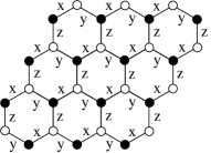
Figure 1: The honeycomb lattice for the Kitaev model. Filled and open circles indicate two sublattices. $x,y,z$ label the links along three different directions used in (1).

Great efforts have been invested to better understand the properties of the Kitaev model. For example, several groups have pointed out that the fractionalized Majorana fermion excitations may be understood from the more familiar Jordan-Wigner transformation of 1D spin systemsXiangT ; ChenHD . The analogy between the non-Abelian Ising vortices and vortices in $p+ip$ superconductors has been raised in serveral worksLeeDH ; YuY ; YuYWangZQ ; Kells . Exact diagonalization has been used to study the Kitaev model on small latticesChenHDProbe . And perturbative expansion methods have been developed to study the gapped phases of the Kitaev-type modelsSchmidt .

Many generalizations of the Kitaev model have been derived as well. There have been several proposals to open the fermion gap for the non-Abelian phase without spoiling exact solvabilityLeeDH ; YuYWangZQ . And many generalizations to other(even 3D) lattices have been developed in the last few yearsHong ; SunCP ; Hong2 ; Nussinov ; Congjun ; Ryu ; Baskaran . All these efforts have significantly enriched our knowledge of exactly solvable models and quantum phases of matter.

However, in the original Kitaev model and its later generalizations in the form of spin models, spin rotation symmetry is explicitly broken. This makes them harder to realize in solid state systems. There are many proposals to realized the Kitaev model in more controllable situations, e.g. in cold atom optical latticesDuanLM ; Micheli , or in superconducting circuitsYouJQ . But it is still desirable for theoretical curiosity and practical purposes to realize the Kitaev-type models in spin rotation invariant systems.

In this paper we realize the Kitaev honeycomb lattice model as the low energy Hamiltonian for a spin rotation invariant system. The trick is not to use the physical spin as the spin in the Kitaev model, instead the spin-1/2 in Kitaev model is from some emergent two-fold degenerate low energy states in the elementary unit of physical system. This type of idea has been explored recently by Jackeli and Khaliullin Khaliullin , in which the spin-1/2 in the Kitaev model is the low energy Kramers doublet created by strong spin-orbit coupling of $t_{2g}$ orbitals. In the model presented below, the Hilbert space of spin-1/2 in the Kitaev model is actually the two dimensional spin singlet sector of four antiferromagnetically coupled spin-1/2 moments, and the role of spin-1/2 operators(Pauli matrices) in the Kitaev model is replaced by certain combinations of ${\bf S}_{j}\cdot{\bf S}_{k}$ [or the spin-chirality ${\bf S}_{j}\cdot({\bf S}_{k}\times{\bf S}_{\ell})$] between the four spins.

One major drawback of the model to be presented is that it contains high order spin interactions(involves up to six or eight spins), thus is still unnatural. However it opens the possibility to realize exotic (exactly solvable) models from spin-1/2 Hamiltonian with spin rotation invariant interactions. We will discuss two possible routes to reduce this artificialness through controlled perturbative expansions, by coupling to optical phonons or by magnetic couplings between the elementary units.

The outline of this paper is as follows. In Section II we will lay out the pseudo-spin-1/2 construction. In Section III the Kitaev model will be explicitly constructed using this formalism, and some properties of this construction will be discussed. In Section IV we will discuss two possible ways to generate the high order spin interactions involved in the construction of Section III by perturbative expansions. Conclusions and outlook will be summarized in Section V.

II Formulation of the Pseudo-spin-1/2 from Four-spin Cluster.

In this Section we will construct the pseudo-spin-1/2 from a cluster of four physical spins, and map the physical spin operators to pseudo-spin operators. The mapping constructed here will be used in later Sections to construct the effective Kitaev model. In this Section we will work entirely within the four-spin cluster, all unspecified physical spin subscripts take values $1,\dots,4$.

Figure 2: Left: the physical spin lattice for the model (8). The dash circles are honeycomb lattice sites, each of which is actually a cluster of four physical spins. The dash straight lines are honeycomb lattice bonds, with their type $x,y,z$ labeled. The interaction between clusters connected by $x,y,z$ bonds are the $J_{x,y,z}$ terms in (8) or (9) respectively. Note this is not the 3-12 lattice used in Ref. Hong ; Schmidt . Right: enlarged picture of the clusters with the four physical spins labeled as $1,\dots,4$. Thick solid bonds within one cluster have large antiferromagnetic Heisenberg coupling $J_{\rm cluster}$.

Consider a cluster of four spin-1/2 moments(called physical spins hereafter), labeled by ${\bf S}_{1,\dots,4}$, antiferromagnetically coupled to each other (see the right bottom part of FIG. 2). The Hamiltonian within the cluster(up to a constant) is simply the Heisenberg antiferromagnetic(AFM) interactions,

$$H_{\rm cluster}=(J_{\rm cluster}/2)\left({\bf S}_{1}+{\bf S}_{2}+{\bf S}_{3}+{\bf S}_{4}\right)^{2}$$ (2)

The energy levels should be apparent from this form: one group of spin-2 quintets with energy $3J_{\rm cluster}$, three groups of spin-1 triplets with energy $J_{\rm cluster}$, and two spin singlets with energy zero. We will consider large positive $J_{\rm cluster}$ limit. So only the singlet sector remains in low energy.

The singlet sector is then treated as a pseudo-spin-1/2 Hilbert space. From now on we denote the pseudo-spin-1/2 operators as ${\bf T}=(1/2)\vec{\tau}$, with $\vec{\tau}$ the Pauli matrices. It is convenient to choose the following basis of the pseudo-spin

$$\begin{split}|\tau^{z}=\pm 1\rangle=\ &\frac{1}{\sqrt{6}}\Big{(}|\downarrow\downarrow\uparrow\uparrow\rangle+\omega^{-\tau^{z}}|\downarrow\uparrow\downarrow\uparrow\rangle+\omega^{\tau^{z}}|\downarrow\uparrow\uparrow\downarrow\rangle\\ \ &\quad+|\uparrow\uparrow\downarrow\downarrow\rangle+\omega^{-\tau^{z}}|\uparrow\downarrow\uparrow\downarrow\rangle+\omega^{\tau^{z}}|\uparrow\downarrow\downarrow\uparrow\rangle\Big{)}\end{split}$$ (3)

where $\omega=e^{2\pi{i}/3}$ is the complex cubic root of unity, $|\downarrow\downarrow\uparrow\uparrow\rangle$ and other states on the right-hand-side(RHS) are basis states of the four-spin system, in terms of $S^{z}$ quantum numbers of physical spins $1,\dots,4$ in sequential order. This pseudo-spin representation has been used by Harris et al. to study magnetic ordering in pyrochlore antiferromagnetsHarris .

We now consider the effect of Heisenberg-type interactions ${\bf S}_{j}\cdot{\bf S}_{k}$ inside the physical singlet sector. Note that since any ${\bf S}_{j}\cdot{\bf S}_{k}$ within the cluster commutes with the cluster Hamiltonian $H_{\rm cluster}$ (2), their action do not mix physical spin singlet states with states of other total physical spin. This property is also true for the spin-chirality operator used later. So the pseudo-spin Hamiltonian constructed below will be exact low energy Hamiltonian, without truncation errors in typical perturbation series expansions.

It is simpler to consider the permutation operators $P_{jk}\equiv 2{\bf S}_{j}\cdot{\bf S}_{k}+1/2$, which just exchange the states of the two physical spin-1/2 moments $j$ and $k$ ($j\neq k$). As an example we consider the action of $P_{34}$,

$$\begin{split}P_{34}|\tau^{z}=-1\rangle=\ &\frac{1}{\sqrt{6}}\Big{(}|\downarrow\downarrow\uparrow\uparrow\rangle+\omega|\downarrow\uparrow\uparrow\downarrow\rangle+\omega^{2}|\downarrow\uparrow\downarrow\uparrow\rangle\\ \ &\quad+|\uparrow\uparrow\downarrow\downarrow\rangle+\omega|\uparrow\downarrow\downarrow\uparrow\rangle+\omega^{2}|\uparrow\downarrow\uparrow\downarrow\rangle\Big{)}\\ =\ &|\tau^{z}=+1\rangle\end{split}$$

and similarly $P_{34}|\tau^{z}=-1\rangle=|\tau^{z}=+1\rangle$. Therefore $P_{34}$ is just $\tau^{x}$ in the physical singlet sector. A complete list of all permutation operators is given in TABLE 1. We can choose the following representation of $\tau^{x}$ and $\tau^{y}$,

$$\begin{split}&\tau^{x}=P_{12}=2{\bf S}_{1}\cdot{\bf S}_{2}+1/2\\ &\tau^{y}=(P_{13}-P_{14})/\sqrt{3}=(2/\sqrt{3}){\bf S}_{1}\cdot({\bf S}_{3}-{\bf S}_{4})\end{split}$$ (4)

Many other representations are possible as well, because several physical spin interactions may correspond to the same pseudo-spin interaction in the physical singlet sector, and we will take advantage of this later.

For $\tau^{z}$ we can use $\tau^{z}=-{i}\tau^{x}\tau^{y}$, where ${i}$ is the imaginary unit,

$$\tau^{z}=-{i}(2/\sqrt{3})(2{\bf S}_{1}\cdot{\bf S}_{2}+1/2){\bf S}_{1}\cdot({\bf S}_{3}-{\bf S}_{4})$$ (5)

However there is another simpler representation of $\tau^{z}$, by the spin-chirality operator $\chi_{jk\ell}={\bf S}_{j}\cdot({\bf S}_{k}\times{\bf S}_{\ell})$. Explicit calculation shows that the effect of ${\bf S}_{2}\cdot({\bf S}_{3}\times{\bf S}_{4})$ is $-(\sqrt{3}/4)\tau^{z}$ in the physical singlet sector. This can also be proved by using the commutation relation $[{\bf S}_{2}\cdot{\bf S}_{3},{\bf S}_{2}\cdot{\bf S}_{4}]={i}{\bf S}_{2}\cdot({\bf S}_{3}\times{\bf S}_{4})$. A complete list of all chirality operators is given in TABLE 1. Therefore we can choose another representation of $\tau^{z}$,

$$\tau^{z}=-\chi_{234}/(\sqrt{3}/4)=-(4/\sqrt{3}){\bf S}_{2}\cdot({\bf S}_{3}\times{\bf S}_{4})$$ (6)

The above representations of $\tau^{x,y,z}$ are all invariant under global spin rotation of the physical spins.

physical spin	pseudo-spin
$P_{12}$, and $P_{34}$	$\tau^{x}$
$P_{13}$, and $P_{24}$	$-(1/2)\tau^{x}+(\sqrt{3}/2)\tau^{y}$
$P_{14}$, and $P_{23}$	$-(1/2)\tau^{x}-(\sqrt{3}/2)\tau^{y}$
$-\chi_{234}$, $\chi_{341}$, $-\chi_{412}$, and $\chi_{123}$	$(\sqrt{3}/4)\tau^{z}$

Table 1: Correspondence between physical spin operators and pseudo-spin operators in the physical spin singlet sector of the four antiferromagnetically coupled physical spins. $P_{jk}=2{\bf S}_{j}\cdot{\bf S}_{k}+1/2$ are permutation operators, $\chi_{jk\ell}={\bf S}_{j}\cdot({\bf S}_{k}\times{\bf S}_{\ell})$ are spin-chirality operators. Note that several physical spin operators may correspond to the same pseudo-spin operator.

With the machinery of equations (4), (5), and (6), it will be straightforward to construct various pseudo-spin-1/2 Hamiltonians on various lattices, of the Kitaev variety and beyond, as the exact low energy effective Hamiltonian of certain spin-1/2 models with spin-rotation symmetry. In these constructions a pseudo-spin lattice site actually represents a cluster of four spin-1/2 moments.

III Realization of the Kitaev Model.

In this Section we will use directly the results of the previous Section to write down a Hamiltonian whose low energy sector is described by the Kitaev model. The Hamiltonian will be constructed on the physical spin lattice illustrated in FIG. 2. In this Section we will use $j,k$ to label four-spin clusters (pseudo-spin-1/2 sites), the physical spins in cluster $j$ are labeled as ${\bf S}_{j1},\dots,{\bf S}_{j4}$.

Apply the mappings developed in Section II, we have the desired Hamiltonian in short notation,

$$\begin{split}H=&\sum_{{\rm cluster}}H_{{\rm cluster}}-\sum_{x-{\rm links}\ <jk>}J_{x}\tau^{x}_{j}\tau^{x}_{k}\\ &-\sum_{y-{\rm links}\ <jk>}J_{y}\tau^{y}_{j}\tau^{y}_{k}-\sum_{z-{\rm links}\ <jk>}J_{z}\tau^{z}_{j}\tau^{z}_{k}\end{split}$$ (7)

where $j,k$ label the honeycomb lattice sites thus the four-spin clusters, $H_{\rm cluster}$ is given by (2), $\tau^{x,y,z}$ should be replaced by the corresponding physical spin operators in (4) and (5) or (6), or some other equivalent representations of personal preference.

Plug in the expressions (4) and (6) into (7), the Hamiltonian reads explicitly as

$$\begin{split}H=\ &\sum_{j}(J_{\rm cluster}/2)({\bf S}_{j1}+{\bf S}_{j2}+{\bf S}_{j3}+{\bf S}_{j4})^{2}-\sum_{z-{\rm links}\ <jk>}J_{z}\,(16/9)[{\bf S}_{j2}\cdot({\bf S}_{j3}\times{\bf S}_{j4})][{\bf S}_{k2}\cdot({\bf S}_{k3}\times{\bf S}_{k4})]\\ \ &-\sum_{x-{\rm links}\ <jk>}J_{x}\,(2{\bf S}_{j1}\cdot{\bf S}_{j2}+1/2)(2{\bf S}_{k1}\cdot{\bf S}_{k2}+1/2)-\sum_{y-{\rm links}\ <jk>}J_{y}\,(4/3)[{\bf S}_{j1}\cdot({\bf S}_{j3}-{\bf S}_{j4})][{\bf S}_{k1}\cdot({\bf S}_{k3}-{\bf S}_{k4})]\end{split}$$ (8)

While by the represenation (4) and (5), the Hamiltonian becomes

$$\begin{split}H=\ &\sum_{j}(J_{\rm cluster}/2)({\bf S}_{j1}+{\bf S}_{j2}+{\bf S}_{j3}+{\bf S}_{j4})^{2}\\ \ &-\sum_{x-{\rm links}\ <jk>}J_{x}\,(2{\bf S}_{j1}\cdot{\bf S}_{j2}+1/2)(2{\bf S}_{k1}\cdot{\bf S}_{k2}+1/2)-\sum_{y-{\rm links}\ <jk>}J_{y}\,(4/3)[{\bf S}_{j1}\cdot({\bf S}_{j3}-{\bf S}_{j4})][{\bf S}_{k1}\cdot({\bf S}_{k3}-{\bf S}_{k4})]\\ \ &-\sum_{z-{\rm links}\ <jk>}J_{z}\,(-4/3)(2{\bf S}_{j3}\cdot{\bf S}_{j4}+1/2)[{\bf S}_{j1}\cdot({\bf S}_{j3}-{\bf S}_{j4})](2{\bf S}_{k3}\cdot{\bf S}_{k4}+1/2)[{\bf S}_{k1}\cdot({\bf S}_{k3}-{\bf S}_{k4})]\end{split}$$ (9)

This model, in terms of physical spins ${\bf S}$, has full spin rotation symmetry and time-reversal symmetry. A pseudo-magnetic field term $\sum_{j}\vec{h}\cdot\vec{\tau}_{j}$ term can also be included under this mapping, however the resulting Kitaev model with magnetic field is not exactly solvable. It is quite curious that such a formidably looking Hamiltonian (8), with biquadratic and six-spin(or eight-spin) terms, has an exactly solvable low energy sector.

We emphasize that because the first intra-cluster term $\sum_{{\rm cluster}}H_{{\rm cluster}}$ commutes with the latter Kitaev terms independent of the representation used, the Kitaev model is realized as the exact low energy Hamiltonian of this model without truncation errors of perturbation theories, namely no $(|J_{x,y,z}|/J_{\rm cluster})^{2}$ or higher order terms will be generated under the projection to low energy cluster singlet space. This is unlike, for example, the $t/U$ expansion of the half-filled Hubbard modelOles ; MacDonald , where at lowest $t^{2}/U$ order the effective Hamiltonian is the Heisenberg model, but higher order terms ($t^{4}/U^{3}$ etc.) should in principle still be included in the low energy effective Hamiltonian for any finite $t/U$. Similar comparison can be made to the perturbative expansion studies of the Kitaev-type models by Vidal et al.Schmidt , where the low energy effective Hamiltonians were obtained in certian anisotropic (strong bond/triangle) limits. Although the spirit of this work, namely projection to low energy sector, is the same as all previous perturbative approaches to effective Hamiltonians.

Note that the original Kitaev model (1) has three-fold rotation symmetry around a honeycomb lattice site, combined with a three-fold rotation in pseudo-spin space (cyclic permutation of $\tau^{x}$, $\tau^{y}$, $\tau^{z}$). This is not apparent in our model (8) in terms of physical spins, under the current representation of $\tau^{x,y,z}$. We can remedy this by using a different set of pseudo-spin Pauli matrices $\tau^{\prime x,y,z}$ in (7),

$$\begin{split}&\tau^{\prime x}=\sqrt{1/3}\tau^{z}+\sqrt{2/3}\tau^{x},\quad\\ &\tau^{\prime y}=\sqrt{1/3}\tau^{z}-\sqrt{1/6}\tau^{x}+\sqrt{1/2}\tau^{y},\\ &\tau^{\prime z}=\sqrt{1/3}\tau^{z}-\sqrt{1/6}\tau^{x}-\sqrt{1/2}\tau^{y}\end{split}$$

With proper representation choice, they have a symmetric form in terms of physical spins,

$$\begin{split}&\tau^{\prime x}=-(4/3){\bf S}_{2}\cdot({\bf S}_{3}\times{\bf S}_{4})+\sqrt{2/3}(2{\bf S}_{1}\cdot{\bf S}_{2}+1/2)\\ &\tau^{\prime y}=-(4/3){\bf S}_{3}\cdot({\bf S}_{4}\times{\bf S}_{2})+\sqrt{2/3}(2{\bf S}_{1}\cdot{\bf S}_{3}+1/2)\\ &\tau^{\prime z}=-(4/3){\bf S}_{4}\cdot({\bf S}_{2}\times{\bf S}_{3})+\sqrt{2/3}(2{\bf S}_{1}\cdot{\bf S}_{4}+1/2)\end{split}$$ (10)

So the symmetry mentioned above can be realized by a three-fold rotation of the honeycomb lattice, with a cyclic permutation of ${\bf S}_{2}$, ${\bf S}_{3}$ and ${\bf S}_{4}$ in each cluster. This is in fact the three-fold rotation symmetry of the physical spin lattice illustrated in FIG. 2. However this more symmetric representation will not be used in later part of this paper.

Another note to take is that it is not necessary to have such a highly symmetric cluster Hamiltonian (2). The mappings to pseudo-spin-1/2 should work as long as the ground states of the cluster Hamiltonian are the two-fold degenerate singlets. One generalization, which conforms the symmetry of the lattice in FIG. 2, is to have

$$H_{\rm cluster}=(J_{\rm cluster}/2)(r\cdot{\bf S}_{1}+{\bf S}_{2}+{\bf S}_{3}+{\bf S}_{4})^{2}$$ (11)

with $J_{\rm cluster}>0$ and $0<r<3$. However this is not convenient for later discussions and will not be used.

We briefly describe some of the properties of (8). Its low energy states are entirely in the space that each of the clusters is a physical spin singlet (called cluster singlet subspace hereafter). Therefore physical spin correlations are strictly confined within each cluster. The excitations carrying physical spin are gapped, and their dynamics are ‘trivial’ in the sense that they do not move from one cluster to another. But there are non-trivial low energy physical spin singlet excitations, described by the pseudo-spins defined above. The correlations of the pseudo-spins can be mapped to correlations of their corresponding physical spin observables (the inverse mappings are not unique, c.f. TABLE 1). For example $\tau^{x,y}$ correlations become certain dimer-dimer correlations, $\tau^{z}$ correlation becomes chirality-chirality correlation, or four-dimer correlation. It will be interesting to see the corresponding picture of the exotic excitations in the Kitaev model, e.g. the Majorana fermion and the Ising vortex. However this will be deferred to future studies.

It is tempting to call this as an exactly solved spin liquid with spin gap ($\sim J_{\rm cluster}$), an extremely short-range resonating valence bond(RVB) state, from a model with spin rotation and time reversal symmetry. However it should be noted that the unit cell of this model contains an even number of spin-1/2 moments (so does the original Kitaev model) which does not satisfy the stringent definition of spin liquid requiring odd number of electrons per unit cell. Several parent Hamiltonians of spin liquids have already been constructed. See for example, Ref. ChayesKivelson ; Batista ; RamanSondhi ; Thomale .

IV Generate the High Order Physical Spin Interactions by Perturbative Expansion.

One major drawback of the present construction is that it involves high order interactions of physical spins[see (8) and (9)], thus is ‘unnatural’. In this Section we will make compromises between exact solvability and naturalness. We consider two clusters $j$ and $k$ and try to generate the $J_{x,y,z}$ interactions in (7) from perturbation series expansion of more natural(lower order) physical spin interactions. Two different approaches for this purpose will be laid out in the following two Subsections. In Subsection IV.1 we will consider the two clusters as two tetrahedra, and couple the spin system to certain optical phonons, further coupling between the phonon modes of the two clusters can generate at lowest order the desired high order spin interactions. In Subsection IV.2 we will introduce certain magnetic, e.g. Heisenberg-type, interactions between physical spins of different clusters, at lowest order(second order) of perturbation theory the desired high order spin interactions can be achieved. These approaches involve truncation errors in the perturbation series, thus the mapping to low energy effect Hamiltonian will no longer be exact. However the error introduced may be controlled by small expansion parameters. In this Section we denote the physical spins on cluster $j$($k$) as $j1,\dots,j4$ ($k1,\dots,k4$), and denote pseudo-spins on cluster $j$($k$) as $\vec{\tau}_{j}$($\vec{\tau}_{k}$).

IV.1 Generate the High Order Terms by Coupling to Optical Phonon.

In this Subsection we regard each four-spin cluster as a tetrahedron, and consider possible optical phonon modes(distortions) and their couplings to the spin system. The basic idea is that the intra-cluster Heisenberg coupling $J_{\rm cluster}$ can linearly depend on the distance between physical spins. Therefore certain distortions of the tetrahedron couple to certain linear combinations of ${\bf S}_{\ell}\cdot{\bf S}_{m}$. Integrating out phonon modes will then generate high order spin interactions. This idea has been extensively studied and applied to several magnetic materialsTchernyshyov ; Mila ; Penc ; Mila2 ; Tchernyshyov2 ; Bergman ; FW . More details can be found in a recent review by Tchernyshyov and ChernTchernyshyovReview . And we will frequently use their notations. In this Subsection we will use the representation (5) for $\tau^{z}$.

Figure 3: Illustration of the tetragonal to orthorhombic $Q^{E}_{1}$(top) and $Q^{E}_{2}$(bottom) distortion modes. (a) Perspective view of the tetrahedron. $1,\dots,4$ label the spins. Arrows indicate the motion of each spin under the distortion mode. (b) Top view of (a). (c)(d) Side view of (a).

Consider first a single tetrahedron with four spins $1,\dots,4$. The general distortions of this tetrahedron can be classified by their symmetry (see for example Ref. TchernyshyovReview ). Only two tetragonal to orthorhombic distortion modes, $Q^{E}_{1}$ and $Q^{E}_{2}$ (illustrated in FIG. 3), couple to the pseudo-spins defined in Section II. A complete analysis of all modes is given in Appendix A. The coupling is of the form

$$J^{\prime}(Q^{E}_{1}f^{E}_{1}+Q^{E}_{2}f^{E}_{2})$$

where $J^{\prime}$ is the derivative of Heisenberg coupling $J_{\rm cluster}$ between two spins $\ell$ and $m$ with respect to their distance $r_{\ell m}$, $J^{\prime}={\rm d}J_{\rm cluster}/{\rm d}r_{\ell m}$; $Q^{E}_{1,2}$ are the generalized coordinates of these two modes; and the functions $f^{E}_{1,2}$ are

$$\begin{split}f^{E}_{2}\ &=(1/2)({\bf S}_{2}\cdot{\bf S}_{4}+{\bf S}_{1}\cdot{\bf S}_{3}-{\bf S}_{1}\cdot{\bf S}_{4}-{\bf S}_{2}\cdot{\bf S}_{3}),\\ f^{E}_{1}\ &=\sqrt{1/12}({\bf S}_{1}\cdot{\bf S}_{4}+{\bf S}_{2}\cdot{\bf S}_{3}+{\bf S}_{2}\cdot{\bf S}_{4}+{\bf S}_{1}\cdot{\bf S}_{3}\\ &\phantom{=\sqrt{1/12}(}-2{\bf S}_{1}\cdot{\bf S}_{2}-2{\bf S}_{3}\cdot{\bf S}_{4}).\end{split}$$

According to TABLE 1 we have $f^{E}_{1}=-(\sqrt{3}/2)\tau^{x}$ and $f^{E}_{2}=(\sqrt{3}/2)\tau^{y}$. Then the coupling becomes

$$(\sqrt{3}/2)J^{\prime}(-Q^{E}_{1}\,\tau^{x}+Q^{E}_{2}\,\tau^{y})$$ (12)

The spin-lattice(SL) Hamiltonian on a single cluster $j$ is [equation (1.8) in Ref. TchernyshyovReview ],

$$\begin{split}H_{{\rm cluster\ }j,{\rm\ SL}}=&H_{{\rm cluster}\ j}+\frac{k}{2}(Q^{E}_{1j})^{2}+\frac{k}{2}(Q^{E}_{2j})^{2}\\ &-\frac{\sqrt{3}}{2}J^{\prime}(Q^{E}_{1j}\tau^{x}_{j}-Q^{E}_{2j}\tau^{y}_{j}),\end{split}$$ (13)

where $k>0$ is the elastic constant for these phonon modes, $J^{\prime}$ is the spin-lattice coupling constant, $Q^{E}_{1j}$ and $Q^{E}_{2j}$ are the generalized coordinates of the $Q^{E}_{1}$ and $Q^{E}_{2}$ distortion modes of cluster $j$, $H_{{\rm cluster}\ j}$ is (2). As already noted in Ref. TchernyshyovReview , this model does not really break the pseudo-spin rotation symmetry of a single cluster.

Now we put two clusters $j$ and $k$ together, and include a perturbation $\lambda\,H_{\rm perturbation}$ to the optical phonon Hamiltonian,

$$\begin{split}H_{jk,{\rm SL}}=&H_{{\rm cluster\ }j,{\rm\ SL}}+H_{{\rm cluster\ }k,{\rm\ SL}}\\ &+\lambda\,H_{\rm perturbation}[Q^{E}_{1j},Q^{E}_{2j},Q^{E}_{1k},Q^{E}_{2k}]\end{split}$$

where $\lambda$ (in fact $\lambda/k$) is the expansion parameter.

Consider the perturbation $H_{\rm perturbation}=Q^{E}_{1j}\cdot Q^{E}_{1k}$, which means a coupling between the $Q^{E}_{1}$ distortion modes of the two tetrahedra. Integrate out the optical phonons, at lowest non-trivial order, it produces a term $(3\,J^{\prime 2}\,\lambda)/(4\,k^{2})\,\tau^{x}_{j}\cdot\tau^{x}_{k}$. This can be seen by minimizing separately the two cluster Hamiltonians with respect to $Q^{E}_{1}$, which gives $Q^{E}_{1}=(\sqrt{3}\,J^{\prime})/(2\,k)\tau^{x}$, then plug this into the perturbation term. Thus we have produced the $J_{x}$ term in the Kitaev model with $J_{x}=-(3\,J^{\prime 2}\,\lambda)/(4\,k^{2})$.

Similarly the perturbation $H_{\rm perturbation}=Q^{E}_{2j}\cdot Q^{E}_{2k}$ will generate $(3\,J^{\prime 2}\,\lambda)/(4\,k^{2})\,\tau^{y}_{j}\cdot\tau^{y}_{k}$ at lowest non-trivial order. So we can make $J_{y}=-(3\,J^{\prime 2}\,\lambda)/(4\,k^{2})$.

The $\tau^{z}_{j}\cdot\tau^{z}_{k}$ coupling is more difficult to get. We treat it as $-\tau^{x}_{j}\tau^{y}_{j}\cdot\tau^{x}_{k}\tau^{y}_{k}$. By the above reasoning, we need an anharmonic coupling $H_{\rm perturbation}=Q^{E}_{1j}Q^{E}_{2j}\cdot Q^{E}_{1k}Q^{E}_{2k}$. It will produce at lowest non-trivial order $(9\,J^{\prime 4}\,\lambda)/(16\,k^{4})\,\tau^{x}_{j}\tau^{y}_{j}\cdot\tau^{x}_{k}\tau^{y}_{k}$. Thus we have $J_{z}=(9\,J^{\prime 4}\,\lambda)/(16\,k^{4})$.

Finally we have made up a spin-lattice model $H_{\rm SL}$, which involves only ${\bf S}_{\ell}\cdot{\bf S}_{m}$ interaction for physical spins,

$$\begin{split}H_{\rm SL}=&\sum_{\rm cluster}H_{{\rm cluster},\ {\rm SL}}+\sum_{x-{\rm links}\ <jk>}\lambda_{x}\,Q^{E}_{1j}\cdot Q^{E}_{1k}\\ &+\sum_{y-{\rm links}\ <jk>}\lambda_{y}\,Q^{E}_{2j}\cdot Q^{E}_{2k}\\ &+\sum_{z-{\rm links}\ <jk>}\lambda_{z}\,Q^{E}_{1j}Q^{E}_{2j}\cdot Q^{E}_{1k}Q^{E}_{2k}\end{split}$$

where $Q^{E}_{1j}$ is the generalized coordinate for the $Q^{E}_{1}$ mode on cluster $j$, and $Q^{E}_{1k}$, $Q^{E}_{2j}$, $Q^{E}_{2k}$ are similarly defined; $\lambda_{x,y}=-(4J_{x,y}k^{2})/(3J^{\prime 2})$ and $\lambda_{z}=(16J_{z}k^{4})/(9J^{\prime 4})$; the single cluster spin-lattice Hamiltonian $H_{{\rm cluster},\ {\rm SL}}$ is (13).

Collect the results above we have the spin-lattice Hamiltonian $H_{\rm SL}$ explicitly written as,

$$\begin{split}H_{\rm SL}=\ &\sum_{{\rm cluster}\ j}\Big{[}(J_{\rm cluster}/2)({\bf S}_{j1}+{\bf S}_{j2}+{\bf S}_{j3}+{\bf S}_{j4})^{2}+\frac{k}{2}(Q^{E}_{1j})^{2}+\frac{k}{2}(Q^{E}_{2j})^{2}\\ &\phantom{\sum_{{\rm cluster}\ j}\Big{[}}+J^{\prime}\Big{(}Q^{E}_{1j}\frac{{\bf S}_{j1}\cdot{\bf S}_{j4}+{\bf S}_{j2}\cdot{\bf S}_{j3}+{\bf S}_{j2}\cdot{\bf S}_{j4}+{\bf S}_{j1}\cdot{\bf S}_{j3}-2{\bf S}_{j1}\cdot{\bf S}_{j2}-2{\bf S}_{j3}\cdot{\bf S}_{j4}}{\sqrt{12}}\\ &\phantom{\sum_{{\rm cluster}\ j}\Big{[}+J^{\prime}\Big{(}}+Q^{E}_{2j}\frac{{\bf S}_{j2}\cdot{\bf S}_{j4}+{\bf S}_{j1}\cdot{\bf S}_{j3}-{\bf S}_{j1}\cdot{\bf S}_{j4}-{\bf S}_{j2}\cdot{\bf S}_{j3}}{2}\Big{)}\Big{]}\\ &-\sum_{x-{\rm links}\ <jk>}\frac{4J_{x}k^{2}}{3J^{\prime 2}}\,Q^{E}_{1j}\cdot Q^{E}_{1k}-\sum_{y-{\rm links}\ <jk>}\frac{4J_{y}k^{2}}{3J^{\prime 2}}\,Q^{E}_{2j}\cdot Q^{E}_{2k}+\sum_{z-{\rm links}\ <jk>}\frac{16J_{z}k^{4}}{9J^{\prime 4}}\,Q^{E}_{1j}Q^{E}_{2j}\cdot Q^{E}_{1k}Q^{E}_{2k}\end{split}$$ (14)

The single cluster spin-lattice Hamiltonian [first three lines in (14)] is quite natural. However we need some harmonic(on $x$- and $y$-links of honeycomb lattice) and anharmonic coupling (on $z$-links) between optical phonon modes of neighboring tetrahedra. And these coupling constants $\lambda_{x,y,z}$ need to be tuned to produce $J_{x,y,z}$ of the Kitaev model. This is still not easy to implement in solid state systems. At lowest non-trivial order of perturbative expansion, we do get our model (9). Higher order terms in expansion destroy the exact solvability, but may be controlled by the small parameters $\lambda_{x,y,z}/k$.

IV.2 Generate the High Order Terms by Magnetic Interactions between Clusters.

In this Subsection we consider more conventional perturbations, magnetic interactions between the clusters, e.g. the Heisenberg coupling ${\bf S}_{j}\cdot{\bf S}_{k}$ with $j$ and $k$ belong to different tetrahedra. This has the advantage over the previous phonon approach for not introducing additional degrees of freedom. But it also has a significant disadvantage: the perturbation does not commute with the cluster Heisenberg Hamiltonian (2), so the cluster singlet subspace will be mixed with other total spin states. In this Subsection we will use the spin-chirality representation (6) for $\tau^{z}$.

Again consider two clusters $j$ and $k$. For simplicity of notations define a projection operator $\mathcal{P}_{jk}=\mathcal{P}_{j}\mathcal{P}_{k}$, where $\mathcal{P}_{j,k}$ is projection into the singlet subspace of cluster $j$ and $k$, respectively, $\mathcal{P}_{j,k}=\sum_{s=\pm 1}|\tau^{z}_{j,k}=s\rangle\langle\tau^{z}_{j,k}=s|$. For a given perturbation $\lambda\,H_{\rm perturbation}$ with small parameter $\lambda$ (in factor $\lambda/J_{\rm cluster}$ is the expansion parameter), lowest two orders of the perturbation series are

$$\begin{split}&\lambda\,\mathcal{P}_{jk}H_{\rm perturbation}\mathcal{P}_{jk}+\lambda^{2}\,\mathcal{P}_{jk}H_{\rm perturbation}(1-\mathcal{P}_{jk})\\ &\times[0-H_{{\rm cluster}\ j}-H_{{\rm cluster}\ k}]^{-1}(1-\mathcal{P}_{jk})H_{\rm perturbation}\mathcal{P}_{jk}\end{split}$$ (15)

With proper choice of $\lambda$ and $H_{\rm perturbation}$ we can generate the desired $J_{x,y,z}$ terms in (8) from the first and second order of perturbations.

The calculation can be dramatically simplified by the following fact that any physical spin-1/2 operator $S^{x,y,z}_{\ell}$ converts the cluster spin singlet states $|\tau^{z}=\pm 1\rangle$ into spin-1 states of the cluster. This can be checked by explicit calculations and will not be proved here. For all the perturbations to be considered later, the above mentioned fact can be exploited to replace the factor $[0-H_{{\rm cluster}\ j}-H_{{\rm cluster}\ k}]^{-1}$ in the second order perturbation to a $c$-number $(-2J_{\rm cluster})^{-1}$.

The detailed calculations are given in Appendix B. We will only list the results here.

The perturbation on $x$-links is given by

$$\begin{split}\lambda_{x}\,H_{{\rm perturbation},\ x}=\ &\lambda_{x}[{\bf S}_{j1}\cdot{\bf S}_{k1}+{\rm sgn}(J_{x})\cdot({\bf S}_{j2}\cdot{\bf S}_{k2})]\\ &-J_{x}({\bf S}_{j1}\cdot{\bf S}_{j2}+{\bf S}_{k1}\cdot{\bf S}_{k2}).\end{split}$$

where $\lambda_{x}=\sqrt{12|J_{x}|\cdot J_{\rm cluster}}$, ${\rm sgn}(J_{x})=\pm 1$ is the sign of $J_{x}$.

The perturbation on $y$-links is

$$\begin{split}&\lambda_{y}\,H_{{\rm perturbation},\ y}\\ =&\lambda_{y}[{\bf S}_{j1}\cdot{\bf S}_{k1}+{\rm sgn}(J_{y})\cdot({\bf S}_{j3}-{\bf S}_{j4})\cdot({\bf S}_{k3}-{\bf S}_{k4})]\\ &-|J_{y}|({\bf S}_{j3}\cdot{\bf S}_{j4}+{\bf S}_{k3}\cdot{\bf S}_{k4})\end{split}$$

with $\lambda_{y}=\sqrt{4|J_{y}|\cdot J_{\rm cluster}}$.

The perturbation on $z$-links is

$$\begin{split}&\lambda_{z}\,H_{{\rm perturbation},\ z}\\ =\ &\lambda_{z}[{\bf S}_{j2}\cdot({\bf S}_{k3}\times{\bf S}_{k4})+{\rm sgn}(J_{z})\cdot{\bf S}_{k2}\cdot({\bf S}_{j3}\times{\bf S}_{j4})]\\ &-|J_{z}|({\bf S}_{j3}\cdot{\bf S}_{j4}+{\bf S}_{k3}\cdot{\bf S}_{k4}).\end{split}$$

with $\lambda_{z}=4\sqrt{|J_{z}|\cdot J_{\rm cluster}}$.

The entire Hamiltonian $H_{\rm magnetic}$ reads explicitly as,

$$\begin{split}&H_{\rm magnetic}=\sum_{{\rm cluster}\ j}(J_{\rm cluster}/2)({\bf S}_{j1}+{\bf S}_{j2}+{\bf S}_{j3}+{\bf S}_{j4})^{2}\\ &\quad+\sum_{x-{\rm links}\ <jk>}\big{\{}\sqrt{12|J_{x}|\cdot J_{\rm cluster}}\big{[}{\bf S}_{j1}\cdot{\bf S}_{k1}+{\rm sgn}(J_{x})\cdot({\bf S}_{j2}\cdot{\bf S}_{k2})\big{]}-J_{x}({\bf S}_{j1}\cdot{\bf S}_{j2}+{\bf S}_{k1}\cdot{\bf S}_{k2})\big{\}}\\ &\quad+\sum_{y-{\rm links}\ <jk>}\big{\{}\sqrt{4|J_{y}|\cdot J_{\rm cluster}}\big{[}{\bf S}_{j1}\cdot({\bf S}_{k3}-{\bf S}_{k4})+{\rm sgn}(J_{y}){\bf S}_{k1}\cdot({\bf S}_{j3}-{\bf S}_{j4})\big{]}-|J_{y}|({\bf S}_{j3}\cdot{\bf S}_{j4}+{\bf S}_{k3}\cdot{\bf S}_{k4})\big{\}}\\ &\quad+\sum_{z-{\rm links}\ <jk>}\big{\{}4\sqrt{|J_{z}|\cdot J_{\rm cluster}}\big{[}{\bf S}_{j2}\cdot({\bf S}_{k3}\times{\bf S}_{k4})+{\rm sgn}(J_{z}){\bf S}_{k2}\cdot({\bf S}_{j3}\times{\bf S}_{j4})\big{]}-|J_{z}|({\bf S}_{j3}\cdot{\bf S}_{j4}+{\bf S}_{k3}\cdot{\bf S}_{k4})\big{\}}.\end{split}$$ (16)

In (16), we have been able to reduce the four spin interactions in (8) to inter-cluster Heisenberg interactions, and the six-spin interactions in (8) to inter-cluster spin-chirality interactions. The inter-cluster Heisenberg couplings in $H_{{\rm perturbation}\ x,y}$ may be easier to arrange. The inter-cluster spin-chirality coupling in $H_{{\rm perturbation}\ z}$ explicitly breaks time reversal symmetry and is probably harder to implement in solid state systems. However spin-chirality order may have important consequences in frustrated magnetsNagaosa ; WenXG , and a realization of spin-chirality interactions in cold atom optical lattices has been proposedTsomokos .

Our model (8) is achieved at second order of the perturbation series. Higher order terms become truncation errors but may be controlled by small parameters $\lambda_{x,y,z}/J_{\rm cluster}\sim\sqrt{|J_{x,y,z}|/J_{\rm cluster}}$.

V Conclusions.

We constructed the exactly solvable Kitaev honeycomb modelKitaev as the exact low energy effective Hamiltonian of a spin-1/2 model [equations (8) or (9)] with spin-rotation and time reversal symmetry. The spin in Kitaev model is represented as the pseudo-spin in the two-fold degenerate spin singlet subspace of a cluster of four antiferromagnetically coupled spin-1/2 moments. The physical spin model is a honeycomb lattice of such four-spin clusters, with certain inter-cluster interactions. The machinery for the exact mapping to pseudo-spin Hamiltonian was developed (see e.g. TABLE 1), which is quite general and can be used to construct other interesting (exactly solvable) spin-1/2 models from spin rotation invariant systems.

In this construction the pseudo-spin correlations in the Kitaev model will be mapped to dimer or spin-chirality correlations in the physical spin system. The corresponding picture of the fractionalized Majorana fermion excitations and Ising vortices still remain to be clarified.

This exact construction contains high order physical spin interactions, which is undesirable for practical implementation. We described two possible approaches to reduce this problem: generating the high order spin interactions by perturbative expansion of the coupling to optical phonon, or the magnetic coupling between clusters. This perturbative construction will introduce truncation error of perturbation series, which may be controlled by small expansion parameters. Whether these constructions can be experimentally engineered is however beyond the scope of this study. It is conceivable that other perturbative expansion can also generate these high order spin interactions, but this possibility will be left for future works.

Appendix A Coupling between Distortions of a Tetrahedron and the Pseudo-spins

In this Appendix we reproduce from Ref. TchernyshyovReview the couplings of all tetrahedron distortion modes to the spin system. And convert them to pseudo-spin notation in the physical spin singlet sector.

Consider a general small distortion of the tetrahedron, the spin Hamiltonian becomes

$$H_{\rm cluster,\ SL}=(J_{\rm cluster}/2)(\sum_{\ell}{\bf S}_{\ell})^{2}+J^{\prime}\sum_{\ell<m}\delta r_{\ell m}({\bf S}_{\ell}\cdot{\bf S}_{m})$$ (17)

where $\delta r_{\ell m}$ is the change of bond length between spins $\ell$ and $m$, $J^{\prime}$ is the derivative of $J_{\rm cluster}$ with respect to bond length.

There are six orthogonal distortion modes of the tetrahedron [TABLE 1.1 in Ref. TchernyshyovReview ]. One of the modes $A$ is the trivial representation of the tetrahedral group $T_{d}$; two $E$ modes form the two dimensional irreducible representation of $T_{d}$; and three $T_{2}$ modes form the three dimensional irreducible representation. The $E$ modes are also illustrated in FIG. 3.

The generic couplings in (17) [second term] can be converted to couplings to these orthogonal modes,

$$J^{\prime}(Q^{A}f^{A}+Q^{E}_{1}f^{E}_{1}+Q^{E}_{2}f^{E}_{2}+Q^{T_{2}}_{1}f^{T_{2}}_{1}+Q^{T_{2}}_{2}f^{T_{2}}_{2}+Q^{T_{2}}_{3}f^{T_{2}}_{3})$$

where $Q$ are generalized coordinates of the corresponding modes, functions $f$ can be read off from TABLE 1.2 of Ref. TchernyshyovReview . For the $A$ mode, $\delta r_{\ell m}=\sqrt{2/3}Q^{A}$, so $f^{A}$ is

$$\begin{split}f^{A}=\ &\sqrt{2/3}\,({\bf S}_{1}\cdot{\bf S}_{2}+{\bf S}_{3}\cdot{\bf S}_{4}+{\bf S}_{1}\cdot{\bf S}_{3}\\ \ &\phantom{\sqrt{2/3}(}+{\bf S}_{2}\cdot{\bf S}_{4}+{\bf S}_{1}\cdot{\bf S}_{4}+{\bf S}_{2}\cdot{\bf S}_{3}).\end{split}$$

The functions $f^{E}_{1,2}$ for the $E$ modes have been given before but are reproduced here,

$$\begin{split}f^{E}_{2}\ &=(1/2)({\bf S}_{2}\cdot{\bf S}_{4}+{\bf S}_{1}\cdot{\bf S}_{3}-{\bf S}_{1}\cdot{\bf S}_{4}-{\bf S}_{2}\cdot{\bf S}_{3}),\\ f^{E}_{1}\ &=\sqrt{1/12}({\bf S}_{1}\cdot{\bf S}_{4}+{\bf S}_{2}\cdot{\bf S}_{3}+{\bf S}_{2}\cdot{\bf S}_{4}+{\bf S}_{1}\cdot{\bf S}_{3}\\ &\phantom{=\sqrt{1/12}(}-2{\bf S}_{1}\cdot{\bf S}_{2}-2{\bf S}_{3}\cdot{\bf S}_{4}).\end{split}$$

The functions $f^{T_{2}}_{1,2,3}$ for the $T_{2}$ modes are

$$\begin{split}f^{T_{2}}_{1}\ &=({\bf S}_{2}\cdot{\bf S}_{3}-{\bf S}_{1}\cdot{\bf S}_{4}),\\ f^{T_{2}}_{2}\ &=({\bf S}_{1}\cdot{\bf S}_{3}-{\bf S}_{2}\cdot{\bf S}_{4}),\\ f^{T_{2}}_{3}\ &=({\bf S}_{1}\cdot{\bf S}_{2}-{\bf S}_{3}\cdot{\bf S}_{4})\end{split}$$

Now we can use TABLE 1 to convert the above couplings into pseudo-spin. It is easy to see that $f^{A}$ and $f^{T_{2}}_{1,2,3}$ are all zero when converted to pseudo-spins, namely projected to the physical spin singlet sector. But $f^{E}_{1}=(P_{14}+P_{23}+P_{24}+P_{13}-2P_{12}-2P_{34})/(4\sqrt{3})=-(\sqrt{3}/2)\tau^{x}$ and $f^{E}_{2}=(P_{24}+P_{13}-P_{14}-P_{23})/4=(\sqrt{3}/2)\tau^{y}$. This has already been noted by Tchernyshyov et al.Tchernyshyov , only the $E$ modes can lift the degeneracy of the physical spin singlet ground states of the tetrahedron. Therefore the general spin lattice coupling is the form of (12) given in the main text.

Appendix B Derivation of the Terms Generated by Second Order Perturbation of Inter-cluster Magnetic Interactions

In this Appendix we derive the second order perturbations of inter-cluster Heisenberg and spin-chirality interactions. The results can then be used to construct (16).

First consider the perturbation $\lambda\,H_{\rm perturbation}=\lambda[{\bf S}_{j1}\cdot{\bf S}_{k1}+r({\bf S}_{j2}\cdot{\bf S}_{k2})]$, where $r$ is a real number to be tuned later. Due to the fact mentioned in Subsection IV.2, the action of $H_{\rm perturbation}$ on any cluster singlet state will produce a state with total spin-1 for both cluster $j$ and $k$. Thus the first order perturbation in (15) vanishes. And the second order perturbation term can be greatly simplified: operator $(1-\mathcal{P}_{jk})[0-H_{{\rm cluster}\ j}-H_{{\rm cluster}\ k}]^{-1}(1-\mathcal{P}_{jk})$ can be replaced by a $c$-number $(-2J_{\rm cluster})^{-1}$. Therefore the perturbation up to second order is

$$-\frac{\lambda^{2}}{2J_{\rm cluster}}\,\mathcal{P}_{jk}(H_{\rm perturbation})^{2}\mathcal{P}_{jk}$$

This is true for other perturbations considered later in this Appendix. The cluster $j$ and cluster $k$ parts can be separated, this term then becomes ($a,b=x,y,z$),

$$\begin{split}&-\frac{\lambda^{2}}{2J_{\rm cluster}}\,\sum_{a,b}\big{[}\mathcal{P}_{j}S^{a}_{j1}S^{b}_{j1}\mathcal{P}_{j}\cdot\mathcal{P}_{k}S^{a}_{k1}S^{b}_{k1}\mathcal{P}_{k}\\ &\quad\quad+2r\,\mathcal{P}_{j}S^{a}_{j1}S^{b}_{j2}\mathcal{P}_{j}\cdot\mathcal{P}_{k}S^{a}_{k1}S^{b}_{k2}\mathcal{P}_{k}\\ &\quad\quad+r^{2}\,\mathcal{P}_{j}S^{a}_{j2}S^{b}_{j2}\mathcal{P}_{j}\cdot\mathcal{P}_{k}S^{a}_{k2}S^{b}_{k2}\mathcal{P}_{k}\big{]}\end{split}$$

Then use the fact that $\mathcal{P}_{j}S^{a}_{j\ell}S^{b}_{jm}\mathcal{P}_{j}=\delta_{ab}(1/3)\mathcal{P}_{j}({\bf S}_{j\ell}\cdot{\bf S}_{jm})\mathcal{P}_{j}$ by spin rotation symmetry, the perturbation becomes

$$\begin{split}&-\frac{\lambda^{2}}{6J_{\rm cluster}}\Big{[}\frac{9+9r^{2}}{16}+2r\,\mathcal{P}_{jk}({\bf S}_{j1}\cdot{\bf S}_{j2})({\bf S}_{k1}\cdot{\bf S}_{k2})\mathcal{P}_{jk}\Big{]}\\ =\ &-\frac{\lambda^{2}}{6J_{\rm cluster}}\Big{[}\frac{9+9r^{2}}{16}+(r/2)\tau^{x}_{j}\tau^{x}_{k}-r/2\\ &\phantom{-\frac{\lambda^{2}}{6J_{\rm cluster}}\Big{[}}-r\,\mathcal{P}_{jk}({\bf S}_{j1}\cdot{\bf S}_{j2}+{\bf S}_{k1}\cdot{\bf S}_{k2})\mathcal{P}_{jk}\Big{]}.\end{split}$$

So we can choose $-(r\,\lambda^{2})/(12J_{\rm cluster})=-J_{x}$, and include the last intra-cluster ${\bf S}_{j1}\cdot{\bf S}_{j2}+{\bf S}_{k1}\cdot{\bf S}_{k2}$ term in the first order perturbation.

The perturbation on $x$-links is then (not unique),

$$\begin{split}\lambda_{x}\,H_{{\rm perturbation},\ x}=&\lambda_{x}[{\bf S}_{j1}\cdot{\bf S}_{k1}+{\rm sgn}(J_{x})\cdot({\bf S}_{j2}\cdot{\bf S}_{k2})]\\ &-J_{x}({\bf S}_{j1}\cdot{\bf S}_{j2}+{\bf S}_{k1}\cdot{\bf S}_{k2})\end{split}$$

with $\lambda_{x}=\sqrt{12|J_{x}|\cdot J_{\rm cluster}}$, and $r={\rm sgn}(J_{x})$ is the sign of $J_{x}$. The non-trivial terms produced by up to second order perturbation will be the $\tau^{x}_{j}\tau^{x}_{k}$ term. Note that the last term in the above equation commutes with cluster Hamiltonians so it does not produce second or higher order perturbations.

Similarly considering the following perturbation on $y$-links, $\lambda\,H_{\rm perturbation}=\lambda[{\bf S}_{j1}\cdot({\bf S}_{k3}-{\bf S}_{k4})+r\,{\bf S}_{k1}\cdot({\bf S}_{j3}-{\bf S}_{j4})]$. Following similar procedures we get the second order perturbation from this term

$$\begin{split}&-\frac{\lambda^{2}}{6J_{\rm cluster}}\Big{[}\frac{9+9r^{2}}{8}\\ &\quad+2r\,\mathcal{P}_{jk}[{\bf S}_{j1}\cdot({\bf S}_{j3}-{\bf S}_{j4})][{\bf S}_{k1}\cdot({\bf S}_{k3}-{\bf S}_{k4})]\mathcal{P}_{jk}\\ &\quad-(3/2)\,\mathcal{P}_{jk}({\bf S}_{k3}\cdot{\bf S}_{k4}+r^{2}\,{\bf S}_{j3}\cdot{\bf S}_{j4})\mathcal{P}_{jk}\Big{]}\\ =\ &-\frac{\lambda^{2}}{6J_{\rm cluster}}\Big{[}\frac{9+9r^{2}}{8}+2r\,(3/4)\tau^{y}_{j}\tau^{y}_{k}\\ &\quad-(3/2)\,\mathcal{P}_{jk}({\bf S}_{k3}\cdot{\bf S}_{k4}+r^{2}\,{\bf S}_{j3}\cdot{\bf S}_{j4})\mathcal{P}_{jk}\Big{]}\end{split}$$

So we can choose $-(r\,\lambda^{2})/(4J_{\rm cluster})=-J_{y}$, and include the last intra-cluster ${\bf S}_{k3}\cdot{\bf S}_{k4}+r^{2}\,{\bf S}_{j3}\cdot{\bf S}_{j4}$ term in the first order perturbation.

Therefore we can choose the following perturbation on $y$-links (not unique),

$$\begin{split}&\lambda_{y}\,H_{{\rm perturbation},\ y}\\ =&\lambda_{y}[{\bf S}_{j1}\cdot{\bf S}_{k1}+{\rm sgn}(J_{y})\cdot({\bf S}_{j3}-{\bf S}_{j4})\cdot({\bf S}_{k3}-{\bf S}_{k4})]\\ &-|J_{y}|({\bf S}_{j3}\cdot{\bf S}_{j4}+{\bf S}_{k3}\cdot{\bf S}_{k4})\end{split}$$

with $\lambda_{y}=\sqrt{4|J_{y}|\cdot J_{\rm cluster}}$, $r={\rm sgn}(J_{y})$ is the sign of $J_{y}$.

The $\tau^{z}_{j}\tau^{z}_{k}$ term is again more difficult to get. We use the representation of $\tau^{z}$ by spin-chirality (6). And consider the following perturbation

$$H_{\rm perturbation}={\bf S}_{j2}\cdot({\bf S}_{j3}\times{\bf S}_{j4})+r\,{\bf S}_{k2}\cdot({\bf S}_{j3}\times{\bf S}_{j4})$$

The first order term in (15) vanishes due to the same reason as before. There are four terms in the second order perturbation. The first one is

$$\begin{split}&\lambda^{2}\,\mathcal{P}_{jk}{\bf S}_{j2}\cdot({\bf S}_{k3}\times{\bf S}_{k4})(1-\mathcal{P}_{jk})\\ &\times[0-H_{{\rm cluster}\ j}-H_{{\rm cluster}\ k}]^{-1}\\ &\times(1-\mathcal{P}_{jk}){\bf S}_{j2}\cdot({\bf S}_{k3}\times{\bf S}_{k4})\mathcal{P}_{jk}\end{split}$$

For the cluster $j$ part we can use the same arguments as before, the $H_{{\rm cluster}\ j}$ can be replaced by a $c$-number $J_{\rm cluster}$. For the cluster $k$ part, consider the fact that ${\bf S}_{k3}\times{\bf S}_{k4}$ equals to the commutator $-{i}[{\bf S}_{k4},{\bf S}_{k3}\cdot{\bf S}_{k4}]$, the action of ${\bf S}_{k3}\times{\bf S}_{k4}$ on physical singlet states of $k$ will also only produce spin-1 state. So we can replace the $H_{{\rm cluster}\ k}$ in the denominator by a $c$-number $J_{\rm cluster}$ as well. Use spin rotation symmetry to separate the $j$ and $k$ parts, this term simplifies to

$$-\frac{\lambda^{2}}{6J_{\rm cluster}}\mathcal{P}_{j}{\bf S}_{j2}\cdot{\bf S}_{j2}\mathcal{P}_{j}\cdot\mathcal{P}_{k}({\bf S}_{k3}\times{\bf S}_{k4})\cdot({\bf S}_{k3}\times{\bf S}_{k4})\mathcal{P}_{k}.$$

Use $({\bf S})^{2}=3/4$ and

$$\begin{split}&({\bf S}_{k3}\times{\bf S}_{k4})\cdot({\bf S}_{k3}\times{\bf S}_{k4})\\ =\ &\sum_{a,b}(S_{k3}^{a}S_{k4}^{b}S_{k3}^{a}S_{k4}^{b}-S_{k3}^{a}S_{k4}^{b}S_{k3}^{b}S_{k4}^{a})\\ =\ &({\bf S}_{k3}\cdot{\bf S}_{k3})({\bf S}_{k4}\cdot{\bf S}_{k4})-\sum_{a,b}S_{k3}^{a}S_{k3}^{b}[\delta_{ab}/2-S_{k4}^{a}S_{k4}^{b}]\\ =\ &9/16+({\bf S}_{k3}\cdot{\bf S}_{k4})({\bf S}_{k3}\cdot{\bf S}_{k4})-(3/8)\end{split}$$

this term becomes

$$\begin{split}&-\frac{\lambda^{2}}{6J_{\rm cluster}}\cdot(3/4)[3/16+(\tau^{x}/2-1/4)^{2}]\\ \ =&-(\lambda^{2})/(32J_{\rm cluster})\cdot(2-\tau^{x}_{k}).\end{split}$$

Another second order perturbation term $r^{2}\lambda^{2}\,\mathcal{P}_{jk}{\bf S}_{k2}\cdot({\bf S}_{j3}\times{\bf S}_{j4})(1-\mathcal{P}_{jk})[0-H_{{\rm cluster}\ j}-H_{{\rm cluster}\ k}]^{-1}(1-\mathcal{P}_{jk}){\bf S}_{k2}\cdot({\bf S}_{j3}\times{\bf S}_{j4})\mathcal{P}_{jk}$ can be computed in the similar way and gives the result $-(r^{2}\,\lambda^{2})/(32J_{\rm cluster})\cdot(2-\tau^{x}_{j})$.

For one of the cross term

$$\begin{split}&r\,\lambda^{2}\,\mathcal{P}_{jk}{\bf S}_{j2}\cdot({\bf S}_{k3}\times{\bf S}_{k4})(1-\mathcal{P}_{jk})\\ &\times[0-H_{{\rm cluster}\ j}-H_{{\rm cluster}\ k}]^{-1}\\ &\times(1-\mathcal{P}_{jk}){\bf S}_{k2}\cdot({\bf S}_{j3}\times{\bf S}_{j4})\mathcal{P}_{jk}\end{split}$$

We can use the previous argument for both cluster $j$ and $k$, so $(1-\mathcal{P}_{AB})[0-H_{{\rm cluster}\ j}-H_{{\rm cluster}\ k}]^{-1}(1-\mathcal{P}_{jk})$ can be replace by $c$-number $(-2J_{\rm cluster})^{-1}$. This term becomes

$$-\frac{r\,\lambda^{2}}{2J_{\rm cluster}}\mathcal{P}_{jk}[{\bf S}_{j2}\cdot({\bf S}_{k3}\times{\bf S}_{k4})][{\bf S}_{k2}\cdot({\bf S}_{j3}\times{\bf S}_{j3})]\mathcal{P}_{jk}.$$

Spin rotation symmetry again helps to separate the terms for cluster $j$ and $k$, and we get $-(r\,\lambda^{2})/(32J_{\rm cluster})\cdot\tau^{z}_{j}\tau^{z}_{k}$.

The other cross term $r\,\lambda^{2}\,\mathcal{P}_{jk}{\bf S}_{k2}\cdot({\bf S}_{j3}\times{\bf S}_{j4})(1-\mathcal{P}_{jk})[0-H_{{\rm cluster}\ j}-H_{{\rm cluster}\ k}]^{-1}(1-\mathcal{P}_{jk}){\bf S}_{j2}\cdot({\bf S}_{k3}\times{\bf S}_{k4})\mathcal{P}_{jk}$ gives the same result.

In summary the second order perturbation from $\lambda[{\bf S}_{j2}\cdot({\bf S}_{j3}\times{\bf S}_{j4})+r\,{\bf S}_{k2}\cdot({\bf S}_{j3}\times{\bf S}_{j4})]$ is

$$-\frac{r\,\lambda^{2}}{16J_{\rm cluster}}\cdot\tau^{z}_{j}\tau^{z}_{k}+\frac{\lambda^{2}}{32J_{\rm cluster}}(\tau^{x}_{k}+r^{2}\,\tau^{x}_{j}-2r^{2}-2).$$

Using this result we can choose the following perturbation on $z$-links,

$$\begin{split}&\lambda_{z}\,H_{{\rm perturbation},\ z}\\ =&\lambda_{z}[{\bf S}_{j2}\cdot({\bf S}_{k3}\times{\bf S}_{k4})+{\rm sgn}(J_{z})\cdot{\bf S}_{k2}\cdot({\bf S}_{j3}\times{\bf S}_{j4})]\\ &-|J_{z}|({\bf S}_{j3}\cdot{\bf S}_{j4}+{\bf S}_{k3}\cdot{\bf S}_{k4})\end{split}$$

with $\lambda_{z}=4\sqrt{|J_{z}|J_{\rm cluster}}$, $r={\rm sgn}(J_{z})$ is the sign of $J_{z}$. The last term on the right-hand-side is to cancel the non-trivial terms $(r^{2}\,\tau^{x}_{j}+\tau^{x}_{k})\lambda_{z}^{2}/(32J_{\rm cluster})$ from the second order perturbation of the first term. Up to second order perturbation this will produce $-J_{z}\tau^{z}_{j}\tau^{z}_{k}$ interactions.

Finally we have been able to reduce the high order interactions to at most three spin terms, the Hamiltonian $H_{\rm magnetic}$ is

$$\begin{split}H_{\rm magnetic}=&\sum_{j}H_{{\rm cluster}\ j}+\sum_{x-{\rm links}\ <jk>}\lambda_{x}H_{{\rm perturbation}\ x}\\ &+\sum_{y-{\rm links}\ <jk>}\lambda_{y}H_{{\rm perturbation}\ y}\\ &+\sum_{z-{\rm links}\ <jk>}\lambda_{z}H_{{\rm perturbation}\ z}\end{split}$$

where $H_{{\rm cluster}\ j}$ are given by (2), $\lambda_{x,y,z}\,H_{{\rm perturbation}\ x,y,z}$ are given above. Plug in relevant equations we get (16) in Subsection IV.2.

References

- (1) Alexei Kitaev, Ann. Phys. (N.Y.) 321, 2 (2006).
- (2) Xiao-Yong Feng, Guang-Ming Zhang, Tao Xiang, Phys. Rev. Lett. 98, 087204 (2007).
- (3) Han-Dong Chen, Zohar Nussinov, J. Phys. A: Math. Theor. 41, 075001 (2008).
- (4) Dung-Hai Lee, Guang-Ming Zhang, Tao Xiang, Phys. Rev. Lett. 99, 196805 (2007).
- (5) Yue Yu, Nucl. Phys. B 799, 345 (2008).
- (6) Yue Yu, Ziqiang Wang, Europhys. Lett. 84, 57002 (2008).
- (7) G. Kells, J. K. Slingerland, J. Vala, Phys. Rev. B 80, 125415 (2009).
- (8) Han-Dong Chen, B. Wang, S. Das Sarma, arXiv:0906.0017 (2009).
- (9) K.P. Schmidt, S. Dusuel, and J. Vidal, Phys. Rev. Lett. 100, 057208 (2008); J. Vidal, K.P. Schmidt, and S. Dusuel, Phys. Rev. B 78, 245121 (2008); S. Dusuel, K.P. Schmidt, J. Vidal, and R.L. Zaffino, Phys. Rev. B 78, 125102 (2008).
- (10) Hong Yao, Steven A. Kivelson, Phys. Rev. Lett. 99, 247203 (2007).
- (11) S. Yang, D. L. Zhou, C. P. Sun, Phys. Rev. B 76, 180404(R) (2007).
- (12) Hong Yao, Shou-Cheng Zhang, Steven A. Kivelson, Phys. Rev. Lett. 102, 217202 (2009).
- (13) Zohar Nussinov, Gerardo Ortiz, Phys. Rev. B 79, 214440 (2009).
- (14) Congjun Wu, Daniel Arovas, Hsiang-Hsuan Hung, Phys. Rev. B 79, 134427 (2009).
- (15) Shinsei Ryu, Phys. Rev. B 79, 075124 (2009).
- (16) G. Baskaran, G. Santhosh, R. Shankar, arXiv:0908.1614 (2009).
- (17) L.-M. Duan, E. Demler, M. D. Lukin, Phys. Rev. Lett. 91, 090402 (2003).
- (18) A. Micheli, G. K. Brennen, P. Zoller, Nature Physics 2, 341 (2006).
- (19) J. Q. You, Xiao-Feng Shi, Xuedong Hu, Franco Nori, Phys. Rev. B 81, 014505 (2010).
- (20) G. Jackeli, G. Khaliullin, Phys. Rev. Lett. 102, 017205 (2009).
- (21) A. B. Harris, A. J. Berlinsky, C. Bruder, J. Appl. Phys. 69, 5200 (1991).
- (22) K. A. Chao, J. Spałek, A. M. Oleś, Phys. Rev. B 18, 3453 (1978).
- (23) A. H. MacDonald, S. M. Girvin, D. Yoshioka, Phys. Rev. B 37, 9753 (1988).
- (24) J. T. Chayes, L. Chayes, S. A. Kivelson, Commun. Math. Phys. 123, 53 (1989).
- (25) C. D. Batista, S. A. Trugman, Phys. Rev. Lett. 93, 217202 (2004).
- (26) K. S. Raman, R. Moessner, S. L. Sondhi, Phys. Rev. B 72, 064413 (2005).
- (27) D. F. Schroeter, E. Kapit, R. Thomale, and M. Greiter, Phys. Rev. Lett. 99, 097202 (2007); R. Thomale, E. Kapit, D. F. Schroeter, and M. Greiter, Phys. Rev. B 80, 104406 (2009).
- (28) O. Tchernyshyov, R. Moessner, S. L. Sondhi, Phys. Rev. Lett. 88, 067203 (2002).
- (29) F. Becca, F. Mila, Phys. Rev. Lett. 89, 037204 (2002).
- (30) K. Penc, N. Shannon, H. Shiba, Phys. Rev. Lett. 93, 197203 (2004).
- (31) C. Weber, F. Becca, F. Mila, Phys. Rev. B 72, 024449 (2005).
- (32) G.-W. Chern, C. J. Fennie, O. Tchernyshyov, Phys. Rev. B 74, 060405(R) (2006).
- (33) D. L. Bergman, R. Shindou, G. A. Fiete, L. Balents, Phys. Rev. B 74, 134409 (2006).
- (34) Fa Wang, Ashvin Vishwanath, Phys. Rev. Lett. 100, 077201 (2008).
- (35) O. Tchernyshyov, G.-W. Chern, arXiv:0907.1693 (2009).
- (36) Y. Taguchi, Y. Oohara, H. Yoshizawa, N. Nagaosa, Y. Tokura, Science 291, 2573 (2001).
- (37) X. G. Wen, Frank Wilczek, A. Zee, Phys. Rev. B 39, 11413 (1989); X. G. Wen, Phys. Rev. B 40, 7387 (1989).
- (38) Dimitris I. Tsomokos, Juan José García-Ripoll, Nigel R. Cooper, Jiannis K. Pachos, Phys. Rev. A 77, 012106 (2008).