Blended General Linear Methods based on
Boundary Value Methods in the
Generalized BDF family

Abstract

Among the methods for solving ODE-IVPs, the class of General Linear Methods (GLMs) is able to encompass most of them, ranging from Linear Multistep Formulae (LMF) to RK formulae. Moreover, it is possible to obtain methods able to overcome typical drawbacks of the previous classes of methods. For example, order barriers for stable LMF and the problem of order reduction for RK methods. Nevertheless, these goals are usually achieved at the price of a higher computational cost. Consequently, many efforts have been made in order to derive GLMs with particular features, to be exploited for their efficient implementation.

In recent years, the derivation of GLMs from particular Boundary Value Methods (BVMs), namely the family of Generalized BDF (GBDF), has been proposed for the numerical solution of stiff ODE-IVPs [11]. In particular, in [8], this approach has been recently developed, resulting in a new family of $L$-stable GLMs of arbitrarily high order, whose theory is here completed and fully worked-out. Moreover, for each one of such methods, it is possible to define a corresponding Blended GLM which is equivalent to it from the point of view of the stability and order properties. These blended methods, in turn, allow the definition of efficient nonlinear splittings for solving the generated discrete problems.

A few numerical tests, confirming the excellent potential of such blended methods, are also reported.

Keywords: Numerical methods for ordinary differential equations, General Linear Methods, Boundary Value Methods (BVMs), Generalized Backward Differentiation Formulae (GBDF), Blended Implicit Methods, blended iteration.

MSC: 65L05, 65L20, 65H10, 65Y20.

1 Introduction

General Linear Methods, in the form introduced by Burrage and Butcher [13], are numerical methods for solving ODE-IVPs which, in order to advance the integration one step, require some information from the previous step (external stages), along with some internal stages to be computed at the current step. Such methods are able to describe, as extreme cases, both RK methods and LMF (the latter, when used as Initial Value Methods (IVMs)) [14]. A GLM with $r$ external stages and $s$ internal stages, when applied with stepsize $h$ for solving the IVP

$$y^{\prime}=f(t,y),\qquad y(t_{0})=y_{0}\in\mathbb{R}^{m},$$ (1)

is usually described as

$$Y^{[n]} = h(A\otimes I_{m})F(Y^{[n]})+(U\otimes I_{m}){\bf y}^{[n-1]},$$ (2)

$${\bf y}^{[n]} = h(B\otimes I_{m})F(Y^{[n]})+(V\otimes I_{m}){\bf y}^{[n-1]},\qquad n=1,2,\dots,$$

where:

• the matrices $A\in\mathbb{R}^{s\times s}$, $U\in\mathbb{R}^{s\times r}$, $B\in\mathbb{R}^{r\times s}$, $V\in\mathbb{R}^{r\times r}$ characterize the method;

• $Y^{[n]},F(Y^{[n]})\in\mathbb{R}^{sm}$ are the vector of the internal stages and the corresponding values of the function $f$, respectively;

• ${\bf y}^{[n-1]},{\bf y}^{[n]}\in\mathbb{R}^{rm}$ are the vectors of the external stages.

Many papers have been devoted, across the years, to the construction and the analysis of GLMs (see, e.g., the review article [16]; see also [15, 17, 18, 19, 20, 21, 22, 23]). Clearly, the efficient implementation of GLMs depends on the properties of the matrix $A$. In particular, we shall here consider implicit GLMs for which the external and the internal stages coincide, i.e.,

$$A=B,~{}U=V\,\in\mathbb{R}^{r\times r},\qquad\mbox{and}\qquad Y^{[n]}={\bf y}^{[n]}\,\in\mathbb{R}^{rm}.$$

Moreover, matrix $A$ is nonsingular and the order of accuracy of each entry of ${\bf y}^{[n]}$ is equal to $p$ (to be specified later), which is, therefore, the global order of the method. We mention that sometimes GLMs with approximations having the same order have been also called “peer methods” (see, e.g., [29]). The approach that we shall consider is the one introduced in [11, Chapter 11, Section 6] and is based on Boundary Value Methods (BVMs). In more detail, the family of BVMs which we shall consider is that of Generalized Backward Differentiation Formulae (GBDF) [10, 11]. For the efficient solution of the generated discrete problems, we shall consider the blended implementation of such methods. This implementation, introduced in [2] for block implicit methods (see also [3, 4, 6, 9, 12]), naturally induces an efficient splitting procedure for the solution of the generated discrete problems. The linear analysis of convergence for this splitting will be done according to [7].

With these premises, the structure of the paper is the following: in Section 2 Boundary Value Methods (BVMs) are briefly sketched, along with their block form; in Section 3 the family of Generalized Backward Differentiation Formulae (GBDF), in the BVMs class, is considered, in order to obtain $L$-stable GLMs of arbitrarily high order; in Section 4 the corresponding Blended GLMs are described; Section 5 is devoted to the implementation details of the methods; Section 6 contains some numerical tests; finally, Section 7 contains a few concluding remarks.

2 Boundary Value Methods (BVMs) and their block form

Boundary Value Methods (BVMs) are a relatively new class of numerical methods for ODEs based on an unconventional use of LMF. Even though recent developments of such methods have been also obtained (see, e.g., [26, 27]), nevertheless, the main reference for such methods remains the book [11]. The basic idea, on which BVMs rely, can be easily explained by just applying a $k$-step LMF, which can be described, by using the usual notation, as

$$\sum_{i=0}^{k}\alpha_{i}y_{n+i}=h\sum_{i=0}^{k}\beta_{i}f_{n+i},$$ (3)

to the standard test equation

$$y^{\prime}=\lambda y,\qquad Re(\lambda)<0.$$ (4)

If we assume we know the first $\nu\in\{1,\dots,k\}$ values of the discrete solution, as well as the last $k-\nu$, say

$$y_{0},\dots,y_{\nu-1},\qquad\mbox{and}\qquad y_{N-k+\nu+1},\dots,y_{N},$$ (5)

then, under suitable conditions for the method, if

$$|z_{1}(q)|\leq|z_{2}(q)|\leq\dots\leq|z_{k}(q)|$$

are the zeros of the characteristic polynomial of the method,

$$\rho(z)-q\sigma(z),~{}~{}\mbox{where}~{}~{}q=h\lambda,~{}~{}\mbox{and}~{}~{}\rho(z)=\sum_{i=0}^{k}\alpha_{i}z^{i},~{}\sigma(z)=\sum_{i=0}^{k}\beta_{i}z^{i},$$ (6)

then the discrete solution is approximately given by

$$y_{n}\approx c\,\left[z_{\nu}(q)\right]^{n},\qquad\mbox{for}\quad 0\ll n\ll N,$$ (7)

with the constant $c$ independent of $N$ [11]. When $\nu=k$ we have the usual way in which LMF are used; i.e., we approximate the continuous IVP by means of a discrete IVP. We speak, in such a case, of an Initial Value Method (IVM). On the other hand, when $\nu<k$ we are approximating the continuous IVP by means of a discrete BVP. The latter defines a Boundary Value Method (BVM) used with $(\nu,k-\nu)$-boundary conditions. This freedom in the choice of the number $\nu$ of the initial conditions in (5), allows us to overcome the usual Dahlquist’s barriers for stable LMF (see [11], for further details).

Nevertheless, the IVP (1) only provides the initial condition $y_{0}$, whereas the remaining set of $k-1$ additional conditions in (5) are not known. However, they can be retrieved implicitly, by introducing a suitable set of $\nu-1$ additional initial methods,

$$\sum_{i=0}^{k}\alpha_{i}^{(j)}y_{i}=h\sum_{i=0}^{k}\beta_{i}^{(j)}f_{i},\qquad j=1,\dots,\nu-1,$$ (8)

and $k-\nu$ additional final methods,

$$\sum_{i=0}^{k}\alpha_{k-i}^{(j)}y_{N-i}=h\sum_{i=0}^{k}\beta_{k-i}^{(j)}f_{N-i},\qquad j=\nu+1,\dots,k,$$ (9)

which are independent of the main method (3). Moreover, in such a way, BVMs can be also implemented in block form (block BVMs [11]), which is computationally more appealing: as a matter of fact, block BVMs have been successfully implemented in the computational codes GAM [24] and GAMD [32]. In more detail, the block method, with blocksize $r$, is used in a sequential fashion by solving, at the $n$th step, a discrete problem in the form

$${\cal A}\otimes I_{m}{\bf y}-h{\cal B}\otimes I_{m}{\bf f}=\bf 0,$$

where

$${\cal A}=\left(\begin{array}[]{ccccccc}\alpha_{0}^{(1)}&\alpha_{1}^{(1)}&\dots&\dots&\alpha_{k}^{(1)}\\ \vdots&\vdots&&&\vdots\\ \alpha_{0}^{(\nu-1)}&\alpha_{1}^{(\nu-1)}&\dots&\dots&\alpha_{k}^{(\nu-1)}\\ \alpha_{0}&\alpha_{1}&\dots&\dots&\alpha_{k}\\ &\ddots&\ddots&&&\ddots\\ &&\alpha_{0}&\alpha_{1}&\dots&\dots&\alpha_{k}\\ &&\alpha_{0}^{(\nu+1)}&\alpha_{1}^{(\nu+1)}&\dots&\dots&\alpha_{k}^{(\nu+1)}\\ &&\vdots&\vdots&&&\vdots\\ &&\alpha_{0}^{(k)}&\alpha_{1}^{(k)}&\dots&\dots&\alpha_{k}^{(k)}\end{array}\right)\in\mathbb{R}^{r\times r+1},$$ (10)

matrix ${\cal B}$ is similarly defined by replacing the $\alpha$-s with the $\beta$-s,

$${\bf y}=(~{}y_{(n-1)r},~{}y_{(n-1)r+1},~{}\dots,~{}y_{nr}~{})^{T},\quad{\bf f}=(~{}f_{(n-1)r},~{}f_{(n-1)r+1},~{}\dots,~{}f_{nr}~{})^{T},$$

and $y_{(n-1)r},f_{(n-1)r}$ are known from the previous step (when $n=1$, $y_{0}$ is the initial condition for problem (1)). Block BVMs allow an easier implementation of variable stepsize, since only the stepsize $h$ of the current “block” can be varied. Several families of block BVMs have then been defined (see [11], for full details).

3 Generalized Backward Differentiation Formulae (GBDF) and GLMs

Let us consider the particular class of $k$-step LMF having the polynomial $\sigma(z)$ in its simplest form, i.e.,

$$\sigma(z)=z^{j},$$

where $j\in\{0,1,\dots,k\}$, with the coefficients of the corresponding polynomial  $\rho(z)$  (see (6)) uniquely defined by imposing that the method has the maximum possible order $p=k$. When $j=k$, one obtains the well-known family of BDF which, however, provides $0$-stable methods only up to $k=6$ and $A$-stable methods up to $k=2$. Nevertheless, when

$$j=\nu\equiv\lceil(k+2)/2\rceil,$$

and the formula is used as a BVM with $(\nu,k-\nu)$-boundary conditions, i.e., by fixing the values (5) of the discrete solution, then it turns out that the resulting methods are stable for all values of $k$, and have been called Generalized BDF (GBDF) [10, 11, 1]. By the way, when $k=1,2$, one obtains the usual first two BDF. In view of the implementation of GBDF as GLMs, one may assume they know the initial values of the discrete solution. On the other hand, the final $k-\nu$ values can be retrieved implicitly by using a suitable set of additional final methods (9), consisting of LMF having the following characteristic polynomials:

$$\sigma^{(j)}(z)=z^{j},\qquad\rho^{(j)}(z)=\sum_{i=0}^{k}\alpha_{i}^{(j)}z^{i},\qquad j=\nu+1,\dots,k,$$

with the coefficients $\{\alpha_{i}^{(j)}\}$ uniquely defined by imposing the order $p=k$ conditions. If we assume, for the sake of simplicity, that a constant stepsize $h$ is used, then by introducing the vectors

$${\bf y}_{new}=\left(\begin{array}[]{c}y_{n+1}\\ \vdots\\ y_{n+r}\end{array}\right),\qquad{\bf f}_{new}=\left(\begin{array}[]{c}f_{n+1}\\ \vdots\\ f_{n+r}\end{array}\right),\qquad{\bf y}_{old}=\left(\begin{array}[]{c}y_{n-r+1}\\ \vdots\\ y_{n}\end{array}\right),$$

and the $r\times r$ matrices ${\cal A}_{1}$ and ${\cal A}_{2}$ such that

$$[{\cal A}_{1}\,|\,{\cal A}_{2}]=\left(\begin{array}[]{ccccc|cccc}&\alpha_{0}&\dots&\dots&\dots&\dots&\alpha_{k}\\ &&\ddots&&&&&\ddots\\ &&&\alpha_{0}&\dots&\dots&\dots&\dots&\alpha_{k}\\ \bf 0&&&\alpha_{0}^{(\nu+1)}&\dots&\dots&\dots&\dots&\alpha_{k}^{(\nu+1)}\\ &&&\vdots&&&&&\vdots\\ &&&\alpha_{0}^{(k)}&\dots&\dots&\dots&\dots&\alpha_{k}^{(k)}\end{array}\right),$$ (11)

it turns out that the discrete problem, at a given point $t_{n}=nh$, can be cast in matrix form as

$$({\cal A}_{2}\otimes I_{m}){\bf y}_{new}=h{\bf f}_{new}-({\cal A}_{1}\otimes I_{m}){\bf y}_{old}.$$ (12)

This corresponds to a GLM of the form (2) with coinciding internal and external stages, and $A={\cal A}_{2}^{-1}$, $U=-{\cal A}_{2}^{-1}{\cal A}_{1}$ (indeed, matrix ${\cal A}_{2}$ turns out to be nonsingular). Such methods were called Block BVMs with Memory (B₂VM₂s) in [11]. In the GLM notation, the abscissae defining this GLM are $c_{i}=i$, $i=1,2,\dots,r$. However, in order to guarantee the $L$-stability of the corresponding method, it is sometimes required to change them into the following set of abscissae:

$$c_{i} = i,\qquad i=1,\dots,\ell-1,$$

$$c_{\ell+j} = \ell-1+\sum_{m=0}^{j}\xi_{m},\qquad j=0,\dots,r-\ell,$$

$$\mbox{with positive}\quad\{\xi_{m}\}\quad\mbox{s.t.}\quad c_{r}=\ell.$$

A first possible choice, as also suggested in [11], is that of setting

$$\xi_{m}=\zeta^{m+1},\qquad m=0,\dots,r-\ell,$$ (14)

where $\zeta$ is the positive root of the polynomial

$$p(z)=\sum_{m=0}^{r-\ell}z^{m+1}-1.$$

However, in general such a value of $\zeta$ is an irrational number, which implies that the coefficients of the corresponding GLM are irrational numbers as well. In order to have methods whose coefficients are always rational numbers, a slightly different choice for the abscissae can be made, i.e.:

$$\xi_{m}=\frac{2^{r-\ell-m}}{2^{r-\ell+1}-1},\qquad m=0,\dots,r-\ell.$$ (15)

Clearly, when  $\ell=r$  we have a uniform mesh, whereas for  $\ell<r$  the last  $r-\ell+1$  stepsizes are geometrically decreasing, in the case of choice (14), or approximately halved, in the case of choice (15). In such a case, the points corresponding to the abscissae  $\{c_{0},\dots,c_{\ell-1},c_{r}\}$  are equally spaced and will be the ones needed for the subsequent integration step. This implies that $r-\ell$ zero columns must be appropriately inserted in matrix ${\cal A}_{1}$ in (11), i.e., those referring to the approximations at the abscissae $\{c_{\ell},\dots,c_{r-1}\}$ (according to [11], such points are called auxiliary points). Consequently, such a GLM based on GBDF is uniquely determined by the triple of integers $(k,r,\ell)$. Clearly, the order of the corresponding method is $p=k$. In addition, for all practical values of $k$, by appropriately choosing the values of $(r,\ell)$, it is possible to guarantee the $L$-stability of such methods. However, it turns out that, for each value of $k$, the couples $(r,\ell)$ are not unique. Consequently, an additional criterion will be considered, in the next section, which is aimed to speed-up the iterative solution of the corresponding discrete problems, via the blended implementation of the methods.

4 Blended General Linear Methods

In the previous section, we devised a procedure for obtaining a whole class of implicit GLMs based on GBDF, containing $L$-stable methods of arbitrarily high order. We now consider the problem of efficiently solving the generated discrete problems which, at a given time step, assume the form (see (2)),

$${\bf y}-h(A\otimes I_{m}){\bf f}=\mbox{\boldmath$\eta$},$$ (16)

where, according to (11) and (12),

$${\bf y}={\bf y}_{new},\qquad{\bf f}={\bf f}_{new},\qquad A={\cal A}_{2}^{-1},\qquad\mbox{\boldmath$\eta$}=-({\cal A}_{2}^{-1}{\cal A}_{1}\otimes I_{m}){\bf y}_{old}.$$

A discrete problem in the form (16) can be efficiently solved, under suitable hypotheses, via the blended implementation of the method. We recall that the blended implementation of block implicit methods has been previously considered in the framework of one-step methods [2, 3, 4, 6, 7, 9, 12] and has been implemented in the computational codes BiM [4, 31] and BiMD [9, 31]. In order to describe the blended implementation of the GLM (16), it is convenient to consider its application for solving the usual test equation (4). In such a case, in fact, the discrete problem reduces to a linear system of dimension $r$:

$$(I-qA){\bf y}=\mbox{\boldmath$\eta$},\qquad q=h\lambda,$$ (17)

where, hereafter, $I$ denotes the identity matrix of dimension $r$. Such a linear system is clearly equivalent to

$$\gamma(A^{-1}-qI){\bf y}=\gamma A^{-1}\mbox{\boldmath$\eta$}\equiv\mbox{\boldmath$\eta$}_{1},$$ (18)

with $\gamma>0$ a free parameter. By introducing the weight function

$$\theta(q)=(1-\gamma q)^{-1}I,$$ (19)

we can then obtain an equivalent discrete problem by combining, with weights $\theta(q)$ and $I-\theta(q)$, respectively, the linear systems (17)-(18):

$$M(q){\bf y} \equiv \left(\theta(q)(I-qA)+\ \gamma(I-\theta(q))(A^{-1}-qI)\right){\bf y}$$ (20)

$$= \theta(q)\mbox{\boldmath$\eta$}+(I-\theta(q))\mbox{\boldmath$\eta$}_{1}~{}\equiv~{}\mbox{\boldmath$\eta$}(q).$$

Equation (20) defines the Blended General Linear Method (Blended GLM) corresponding to the original GLM (17). Then, in view of the fact that

$$M(q)\approx\left\{\begin{array}[]{cl}I,&\mbox{for}\quad q\approx 0,\\[5.69054pt] -\gamma qI,&\mbox{for}\quad|q|\gg 1,\end{array}\right.$$

the following blended iteration for solving the discrete problem (20) is naturally induced:

$$N(q){\bf y}^{(i+1)}\equiv(I-\gamma qI){\bf y}^{(i+1)}=(N(q)-M(q)){\bf y}^{(i)}+\mbox{\boldmath$\eta$}(q),\qquad i=0,1,\dots.$$ (21)

Remark 1

By considering that in (21) $N(q)^{-1}=\theta(q)$ (see (19)), it is quite straightforward to realize that, in the case of problem (1), the corresponding blended iteration formally becomes

$$\mbox{\boldmath$\delta$}^{(i)} = N^{-1}\left(\theta\left((I-\gamma A^{-1})\otimes I_{m}\,({\bf y}^{(i)}-\mbox{\boldmath$\eta$})-h(A-\gamma I)\otimes I_{m}{\bf f}^{(i)}\right)\right.$$ (22)

$$\left.+\gamma\left(A^{-1}\otimes I_{m}\,({\bf y}^{(i)}-\mbox{\boldmath$\eta$})-hI\otimes I_{m}\,{\bf f}^{(i)}\right)\right),$$

$${\bf y}^{(i+1)} = {\bf y}^{(i)}-\mbox{\boldmath$\delta$}^{(i)},\qquad i=0,1,\dots,$$

where

$$N\equiv\theta^{-1}=I\otimes(I_{m}-h\gamma J),$$ (23)

with $J$ the Jacobian of $f$ evaluated at the last known point. Consequently, only the factorization of one matrix of the size of the continuous problem is required.

Coming back to the iteration (21), we observe that (see [3, 7]) the iteration matrix corresponding to the blended iteration (21) turns out to be given by

$$Z(q)\equiv I-N(q)^{-1}M(q)=\frac{q}{(1-\gamma q)^{2}}A^{-1}(A-\gamma I)^{2}.$$ (24)

According to the linear analysis described in [7], we shall now study the spectral properties of $Z(q)$, in order to obtain a linear analysis of convergence for the iteration (21). For this purpose, hereafter let $\rho(q)$ denote the spectral radius of $Z(q)$. Clearly, the iteration will be convergent if and only if $\rho(q)<1$; moreover, the set

$$\Gamma=\left\{q\in\mathbb{C}\,:\,\rho(q)<1\right\}$$

is the region of convergence of the iteration. For the sake of completeness (see [7] for details), we recall that the iteration is:

• $0$-convergent, if $\rho(0)=0$;

• $A$-convergent, if $\mathbb{C}^{-}\subseteq\Gamma$;

• $L$-convergent with index $\nu_{\infty}$, if it is $A$-convergent,

  $$Z_{\infty}\equiv\lim_{q\rightarrow\infty}Z(q)=O,$$

  and $\nu_{\infty}$ is the index of nilpotency of $Z_{\infty}$.

Clearly, the iteration (21) is $0$-convergent, since $Z(0)=O$. Moreover, one easily verifies (from (24)) that

$$Z(q)\rightarrow O,\quad\mbox{as}\quad q\rightarrow\infty,$$

so that $A$-convergence and $L$-convergence (with index 1) are equivalent. In addition to this,

$$\rho(q)\approx\left\{\begin{array}[]{ll}\approx\tilde{\rho}q,&\mbox{for}\quad q\approx 0,\\[5.69054pt] \approx\tilde{\rho}_{\infty}q^{-1},&\mbox{for}\quad|q|\gg 1,\end{array}\right.$$

where $\tilde{\rho}$ and $\tilde{\rho}_{\infty}$ are the nonstiff amplification factor and the stiff convergence factor of the iteration, respectively. Finally, for a $0$-convergent iteration, $A$-convergence is equivalent to requiring that the maximum amplification factor,

$$\rho^{*}=\max_{x>0}\rho(ix),$$

(with $i$ denoting, as usual, the imaginary unit) is not greater than 1. According to [7], $\tilde{\rho}$, $\tilde{\rho}_{\infty}$, and $\rho^{*}$ are evaluation parameters for the blended iteration (21) (the smaller they are, the better the properties of the iteration). Consequently, if $\rho^{*}\leq 1$, the iteration is $L$-convergent and, therefore, appropriate for $L$-stable methods [7], like the GLMs defined in Section 3.

Because of the form (24) of the iteration matrix, it turns out that (see also [7]):

$$\tilde{\rho}=\rho\left(A^{-1}(A-\gamma I)^{2}\right),\qquad\tilde{\rho}_{\infty}=\gamma^{-2}\tilde{\rho},\qquad\rho^{*}=(2\gamma)^{-1}\tilde{\rho},$$

with $\rho\left(A^{-1}(A-\gamma I)^{2}\right)$ denoting the spectral radius of that matrix. Consequently, the value of the free positive parameter $\gamma$ is chosen in order to minimize $\rho^{*}$. In Table 2, the relevant figures are reported for selected GLMs based on GBDF, each characterized by the corresponding triple $(k,r,\ell)$, when the choice (14) for the auxiliary points is considered. Similarly, in Table 2, the same results, obtained with the choice (15) of the auxiliary points, are listed. In both tables, we list $r-\ell$ (i.e., the number of the auxiliary points) in place of $\ell$. The specified values of the blocksize $r$, have been here chosen as small as possible, in order to minimize the computational cost per step.

As it can be seen, the blended iteration corresponding to each method turns out to be $L$-convergent. Moreover, the value of the parameter $\gamma$ (with the only exception of that corresponding to $k=4$, for both the choices of the auxiliary steps) turns out to coincide with the value

$$\gamma^{*}=\min_{\mu\in\sigma(A)}|\mu|,$$

suggested in [3] for a class of Blended Implicit Methods (see also [7]).

As an example, we list the matrices $A$ and $U$ which define the third order GLM corresponding to the triple $(3,2,2)$, requiring no auxiliary steps (hereafter, let ${\bf c}\in\mathbb{R}^{r}$ denote the vector of the abscissae),

$${\bf c}=(\,1,\,2\,)^{T},\qquad A=\frac{1}{23}\left(\begin{array}[]{rr}22&-4\\ 36&6\end{array}\right),\qquad U=\frac{1}{23}\left(\begin{array}[]{rr}-5&28\\ -4&27\end{array}\right),$$ (25)

and those defining the fourth order GLM corresponding to the triple $(4,4,3)$, with the choice (14),

$${\bf c}=\left(\,1,\,2,\,\frac{3+\sqrt{5}}{2},\,3\,\right)^{T},$$

$$A=$$

$${\small\left(\begin{array}[]{rrrr}0.85795933248329&-0.22588594615620&0.09292560797716&-0.02384741384935\\ 1.14013555838905&0.75295315385401&-0.30975202659054&0.07949137949784\\ 1.16454145194449&0.91413597782316&0.27338586108581&-0.07015876367984\\ 1.16304178987375&0.90057211551936&0.50490826434742&0.09507592794253\end{array}\right)},$$

$$U={\small\left(\begin{array}[]{rrrr}0.07149661104027&-0.44184164162566&0&1.37034503058538\\ 0.09501129653242&-0.52719452791448&0&1.43218323138206\\ 0.09704512099537&-0.53021970356702&0&1.43317458257165\\ 0.09692014915615&-0.53024220062923&0&1.43332205147308\end{array}\right)}.$$

and with the choice (15),

$${\bf c} = \left(\,1,\,2,\,\frac{8}{3},\,3\,\right)^{T},$$

$$A = \frac{1}{6336684}\,\left(\begin{array}[]{rrrr}5429268&-1381941&570807&-174960\\ 7249176&4606470&-1902690&583200\\ 7421568&5690784&2388672&-732160\\ 7415388&5637357&3628233&198936\end{array}\right),$$

$$U = \frac{1}{6336684}\,\left(\begin{array}[]{rrrr}452439&-2798388&0&8682633\\ 604098&-3345408&0&9077994\\ 618464&-3365888&0&9084108\\ 617949&-3366036&0&9084771\end{array}\right),$$

which slightly differ from each other.

$k$ $r$ $r-\ell$ $\gamma$ $\tilde{\rho}$ $\tilde{\rho}_{\infty}$ $\rho^{*}$ 3 2 0 0.7223 0.2272 0.4355 0.1573 4 4 1 0.6195 0.3802 0.9908 0.3069 6 5 1 0.6063 0.5734 1.5600 0.4729 8 6 1 0.5769 0.6380 1.9170 0.5530 10 7 1 0.5502 0.6626 2.1887 0.6021 12 9 2 0.5271 0.7345 2.6438 0.6968 14 10 2 0.5127 0.7366 2.8022 0.7183 16 11 2 0.4999 0.7345 2.9393 0.7347

Table 1: Parameters of the blended iteration associated with Blended GLMs, based on GBDF, characterized by the triple $(k,r,\ell)$ and the choice (14).

$k$ $r$ $r-\ell$ $\gamma$ $\tilde{\rho}$ $\tilde{\rho}_{\infty}$ $\rho^{*}$ 3 2 0 0.7223 0.2272 0.4355 0.1573 4 4 1 0.6249 0.3827 0.9801 0.3062 6 5 1 0.6082 0.5740 1.5520 0.4719 8 6 1 0.5778 0.6381 1.9113 0.5522 10 7 1 0.5507 0.6625 2.1845 0.6015 12 9 2 0.5274 0.7345 2.6407 0.6964 14 10 2 0.5130 0.7366 2.7998 0.7180 16 11 2 0.5000 0.7345 2.9374 0.7344

Table 2: Parameters of the blended iteration associated with Blended GLMs, based on GBDF, characterized by the triple $(k,r,\ell)$ and the choice (15).

Finally, in Figures 2 and 2, we plot the boundary of the stability regions of the methods listed in Table 2, whereas in Figures 4 and 4, we plot the boundary of the stability regions of the methods listed in Table 2.

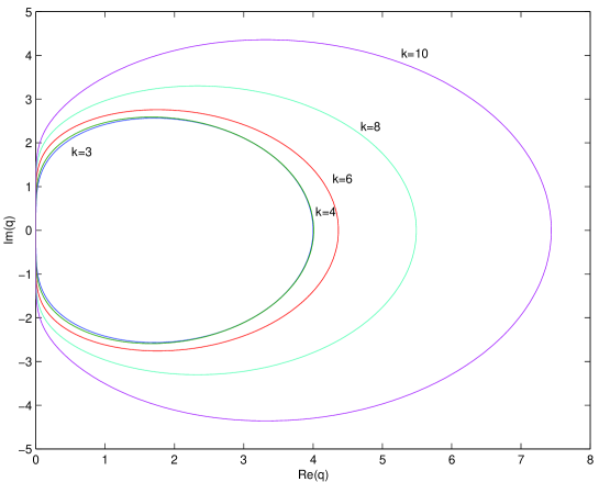
Figure 1: Boundary loci of the GLMs obtained with the choice (14), $k=3,4,6,8,10$.

Figure 2: Boundary loci of the GLMs obtained with the choice (14), $k=12,14,16$.

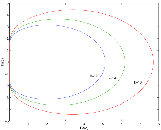
Figure 3: Boundary loci of the GLMs obtained with the choice (15), $k=3,4,6,8,10$.

Figure 4: Boundary loci of the GLMs obtained with the choice (15), $k=12,14,16$.

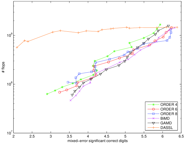
Figure 5: Numerical results for the Pollution Problem.

Figure 6: Numerical results for the Elastic Beam Problem.

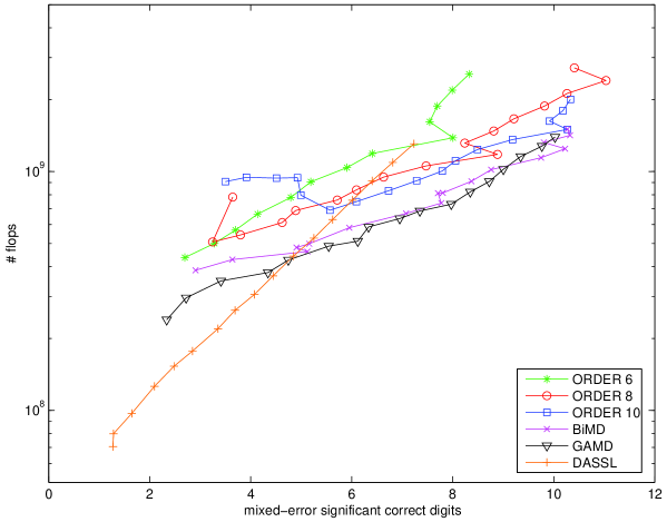
Figure 7: Numerical results for the Emep Problem.

Figure 8: Numerical results for the Ring Modulator Problem.

5 Implementation details

In the actual implementation of the above Blended GLMs, three main points need to be clarified:

• the choice of a suitable starting procedure;

• an efficient local error estimate;

• the variable stepsize implementation of the methods.

All of them are briefly sketched here.

Concerning the first issue, namely the definition of a starting procedure to obtain the first vector of approximations, from the initial condition $y_{0}$ of problem (1), a natural candidate is the block GBDF of order $k$ and blocksize $r=k$. In more detail, at the very beginning, one solves the discrete problem

$${\cal A}\otimes I_{m}{\bf y}-h{\cal B}\otimes I_{m}{\bf f}=\bf 0,$$ (30)

where

$${\bf y}=(~{}y_{0},~{}y_{1},~{}\dots,~{}y_{k}~{})^{T},\qquad{\bf f}=(~{}f_{0},~{}f_{1},~{}\dots,~{}f_{k}~{})^{T},$$

and, by denoting with $\{\alpha_{i}^{(j)}\}$ the $\alpha$-s coefficients of the additional initial and final methods (8) and (9), the matrices ${\cal A}$ and ${\cal B}$ are defined as (see (10)):

$${\cal A}=\left(\begin{array}[]{l|lcl}\alpha_{0}^{(1)}&\alpha_{1}^{(1)}&\dots&\alpha_{k}^{(1)}\\ \vdots&\vdots&&\vdots\\ \alpha_{0}^{(\nu-1)}&\alpha_{1}^{(\nu-1)}&\dots&\alpha_{k}^{(\nu-1)}\\ \alpha_{0}&\alpha_{1}&\dots&\alpha_{k}\\ \alpha_{0}^{(\nu+1)}&\alpha_{1}^{(\nu+1)}&\dots&\alpha_{k}^{(\nu+1)}\\ \vdots&\vdots&&\vdots\\ \alpha_{0}^{(k)}&\alpha_{1}^{(k)}&\dots&\alpha_{k}^{(k)}\end{array}\right),~{}{\cal B}=(\,{\bf 0}\,|\,I_{k}\,)~{}\in~{}\mathbb{R}^{k\times k+1}.$$

For the efficient solution of equation (30), a corresponding blended methods, with the associated blended iteration, can be conveniently and easily defined.

The estimate of the local error is obtained by deferred correction, as described in [11, Chapter 10] (see also [4, 5]), by first “plugging” the local discrete solution (see (12)) $(\,{\bf y}_{old},\,{\bf y}_{new}\,)^{T}$ in the discrete problem defined by a higher order method. In such a way, one obtains an estimate $\tau$ of the local truncation error. The same is done by considering an equivalent formulation of the same method (compare with (16) and (17)-(18)), thus obtaining a new approximation $\mbox{\boldmath$\tau$}_{1}=\gamma A^{-1}\otimes I_{m}\mbox{\boldmath$\tau$}$. After that, the estimate ${\bf e}$ of the local error is obtained by performing one blended iteration, namely by formally solving the block diagonal linear system (see (23))

$$N{\bf e}=\theta\mbox{\boldmath$\tau$}+(I-\theta)\mbox{\boldmath$\tau$}_{1}.$$

In more detail, when using the GLM defined by the triple $(k,r,\ell)$, the corresponding method used for estimating $\tau$ is the GBDF defined by the triple $(k+1,r,\ell)$. Consequently, the cost for estimating ${\bf e}$ is the same as that for carrying out one blended iteration. This can be done for all methods listed in Tables 2 and 2, with the only exception being the triple (3,2,2), for which the value of $r$ should be increased. For this reason, such a method has not been considered for carrying out the numerical tests in Section 6.

Finally, for the efficient variation of the stepsize, we have considered the Nordsiek implementation of the methods, firstly introduced in [28] and later modified according to, e.g., [25, 30]. For the sake of completeness, we also mention that the initial guess for the blended iteration (22)-(23) is obtained by extrapolation, through the interpolating polynomial on (see (12)) ${\bf y}_{old}$.

6 Numerical Tests

In this section, we report a few numerical tests comparing a Matlab fixed-order implementation of the Blended GLMs presented here, with some of the most reliable codes currently available, on selected stiff test problems. Both the problems and the codes have been taken from the current release (release 2.4) of Test Set for IVP Solvers [32]. In particular, we have considered the following solvers:

• BiMD, which uses a blended iteration for solving the generated discrete problems;

• GAMD, which uses a nonlinear splitting for solving the discrete problems, generated by block BVMs in the Generalized Adams Methods (GAMs) family;

• DASSL, which implements standard BDF methods.

The problems considered are:

• Pollution (of dimension 20);

• Elastic Beam (of dimension 80);

• Emep (of dimension 66);

• Ring Modulator (of dimension 15).

The comparisons have been summarized in corresponding work-precision diagrams [32], where the computational cost is plotted versus accuracy. A standardized cost has been computed as the number of floating-point operations for the factorizations and the system solvings required by each code, while accuracy has been measured in terms of mixed-error significant correct digits [32]. For all codes, the used tolerances are essentially those specified in the Test Set. Figures 6–8 summarize the results obtained, where the label “ORDER $k$” is used for the fixed-order implementation of the Blended GBDF of order $k$ (see Table 2): as one can see, for each problem, the selected fixed-order implementations of the Blended GBDF presented here, appear to be competitive with the above mentioned solvers.

7 Conclusions

In this paper, a straightforward approach for deriving $L$-stable General Linear Methods (GLMs) of arbitrarily high order has been presented. Such an approach relies on the class of Boundary Value Methods (BVMs) for ODEs. In the same framework corresponding starting procedures are easily derived, as well as appropriate error estimates.

The generated discrete problems can be efficiently solved by means of the blended implementation of the methods, thus defining corresponding Blended GLMs, equivalent to the original methods, from the point of view of the stability and accuracy properties. The corresponding blended iterations are all $L$-convergent, thus appropriate for the underlying $L$-stable methods.

A number of numerical tests, on problems taken from the Test Set for IVP Solvers, prove that the obtained methods are competitive with some of the best codes currently available.

The availability of methods having arbitrarily high-order makes them good candidates for an efficient variable-order implementation.

References

- [1] L. Aceto, D. Trigiante. On the -stable methods in the GBDF class. Nonlinear Anal. Real World Appl. 3 (2002) 9–23.
- [2] L. Brugnano. Blended Block BVMs (B3VMs): a family of economical implicit methods for ODEs. Jour. Comput. Appl. Mathematics 116 (2000) 41–62.
- [3] L. Brugnano, C. Magherini. Blended Implementation of Block Implicit Methods for ODEs. Appl. Numer. Math. 42 (2002) 29–45.
- [4] L. Brugnano, C. Magherini. The BiM code for the numerical solution of ODEs. Jour. Comput. Appl. Mathematics 164–165 (2004) 145–158.
- [5] L. Brugnano, C. Magherini. Economical Error Estimates for Block Implicit Methods for ODEs via Deferred Correction. Appl. Numer. Math. 56 (2006) 608–617.
- [6] L. Brugnano, C. Magherini. Blended Implicit Methods for solving ODE and DAE problems, and their extension for second order problems. Jour. Comput. Appl. Mathematics 205 (2007) 777–790
- [7] L. Brugnano, C. Magherini. Recent advances in linear analysis of convergence for splittings for solving ODE problems. Appl. Numer. Math. 59 (2009) 542–557.
- [8] L. Brugnano, C. Magherini. Blended General Linear Methods based on Generalized BDF. AIP Conference Proceedings 1048 (2008) 871–874.
- [9] L. Brugnano, C. Magherini, F. Mugnai. Blended Implicit Methods for the numerical solution of DAE problems. Jour. Comput. Appl. Mathematics 189 (2006) 34–50.
- [10] L. Brugnano, D. Trigiante. Convergence and stability of Boundary Value Methods for ordinary differential equations. Jour. Comput. Appl. Mathematics 66 (1996) 97–109.
- [11] L.Brugnano, D.Trigiante. Solving Differential Problems by Multistep Initial and Boundary Value Methods, Gordon and Breach Science Publ., 1998.
- [12] L. Brugnano, D. Trigiante. Block Implicit Methods for ODEs, in Recent Trends in Numerical Analysis, D.Trigiante ed., Nova Science Publ. Inc., New York, 2001, pp. 81-105.
- [13] K. Burrage, J.C. Butcher. Non-linear stability of a general class of differential equation methods. BIT 20 (1980) 185–203.
- [14] J.C. Butcher. The Numerical Analysis of Ordinary Differential Equations. Runge-Kutta and General Linear Methods, John Wiley, New York, 1987.
- [15] J.C. Butcher. Diagonally-implicit multi-stage integration methods. Appl. Numer. Math. 11 (1993) 347–363.
- [16] J.C. Butcher. General linear methods. Acta Numerica 15 (2006) 157–256.
- [17] J.C. Butcher, P. Chartier, Z. Jackiewicz. Nordsieck representation of DIMSIMs. Numer. Alg. 16 (1997) 209–230.
- [18] J.C. Butcher, Z. Jackiewicz. Diagonally implicit general linear methods for ordinary differential equations. BIT 33 (1993) 452–472.
- [19] J.C. Butcher, Z. Jackiewicz. Construction of diagonally implicit general linear methods of type 1 and 2 for ordinary differential equations. Appl. Numer. Math. 21 (1996) 385–415.
- [20] J.C. Butcher, Z. Jackiewicz. Construction of high order diagonally implicit multistage integration methods for ordinary differential equations. Appl. Numer. Math. 27 (1998) 1–12.
- [21] J.C. Butcher, Z. Jackiewicz. Construction of general linear methods with Runge-Kutta stability properties. Numer. Alg. 36 (2004) 53–72.
- [22] J.C. Butcher, Z. Jackiewicz, H.D. Mittelmann. Nonlinear optimization approach to the construction of general linear methods of high order. Jour. Comput. Appl. Math. 81 (1997) 181–196.
- [23] J.C. Butcher, W.M. Wright. The construction of practical general linear methods. BIT 43 (2003) 695–721.
- [24] F. Iavernaro, F. Mazzia. Solving Ordinary Differential Equations by Generalized Adams Methods: properties and implementation techniques. Appl. Num. Math. 28 (1998) 107–126.
- [25] J.D. Lambert. Numerical Methods for Ordinary Differential Equations, John Wiley & Sons, Chichester, 1993.
- [26] F. Mazzia, A. Sestini, D. Trigiante. B-spline multistep methods and their continuous extensions. SIAM Jour. Numer. Anal. 44 (2006) 1954–1973.
- [27] F. Mazzia, A. Sestini, D. Trigiante. Bs linear multistep methods on non uniform mesh. Jour. Numer. Anal., Industrial and Appl. Math. 1 (2006) 91–112.
- [28] A. Nordsiek. On Numerical Integration of Ordinary Differential Equations. Math. Comp. 16 (1962) 22–49.
- [29] H. Podhaisky, R. Weiner, B.A. Schmitt. Linearly-implicit two-step methods and their implementation in Nordsieck form. Appl. Numer. Math. 56 (2006) 374–387.
- [30] K. Radhakrishnan, A. Hindmarsh. Description and Use of LSODE, the Livermore Solver for Ordinary Differential Equations. LLNL Report UCRL-ID-113855, 1993.
-
[31]
Codes BiM and BiMD homepage:
http://www.math.unifi.it/~brugnano/BiM - [32] Test Set for IVP Solvers: http://pitagora.dm.uniba.it/~testset