Instrument Performance in Kepler’s First Months
Abstract
The Kepler Mission relies on precise differential photometry to detect the 80 parts per million (ppm) signal from an Earth--Sun equivalent transit. Such precision requires superb instrument stability on time scales up to 2 days and systematic error removal to better than 20 ppm. To this end, the spacecraft and photometer underwent 67 days of commissioning, which included several data sets taken to characterize the photometer performance. Because Kepler has no shutter, we took a series of dark images prior to the dust cover ejection, from which we measured the bias levels, dark current, and read noise. These basic detector properties are essentially unchanged from ground-based tests, indicating that the photometer is working as expected. Several image artifacts have proven more complex than when observed during ground testing, as a result of their interactions with starlight and the greater thermal stability in flight, which causes the temperature-dependent artifact variations to be on the timescales of transits. Because of Kepler’s unprecedented sensitivity and stability, we have also seen several unexpected systematics that affect photometric precision. We are using the first 43 days of science data to characterize these effects and to develop detection and mitigation methods that will be implemented in the calibration pipeline. Based on early testing, we expect to attain Kepler’s planned photometric precision over 80%--90% of the field of view.
Subject headings:
instrumentation: photometers --- planetary systems --- space vehicles: instruments --- techniques: photometric1. Introduction
Kepler was launched on 2009 March 6, beginning a 3 1/2 year mission to detect transiting exoplanets and determine the frequency of Earth-size planets in the habitable zones of solar-like stars. The objectives and early results of the Kepler Mission are reviewed by Borucki, et al. (2010) and the mission design and overall performance are reviewed by Koch et al. (2010). Before beginning science operations, Kepler underwent a commissioning period to ensure it was operating correctly after the rigors of launch, to verify that ground-based characterizations were still valid, and to perform characterizations that could only be done in space (Haas et al., 2010). In this Letter we describe the instrument characteristics relevant for understanding Kepler’s raw pixel data. In addition to standard CCD detector properties (§ 3.1), we discuss the characterizations and data products resulting from Kepler’s unique design and operation (§ 3.2). In § 4, we describe several image artifacts that are present in Kepler data and discuss their impact on photometric precision. Detailed descriptions of the photometer beyond the scope of this Letter can be found in Argabright et al. (2008) and in the ‘‘Kepler Instrument Handbook’’ (Van Cleve & Caldwell, 2009).
2. Observation Modes
Kepler science data are available at either short cadence (1 minute) for 512 targets, or long cadence (30 minutes) for 170,000 targets. All science data are collected with an integration time of 6.02 s. In science collection mode, the full single integration CCD frames are coadded together, then at the end of the short and long cadence period pre-specified pixels for each target are selected from the coadd, processed, and stored on board. Due to data storage and transmission limitations, only about 6% of the 96 million pixels are stored for eventual transmission to the ground.
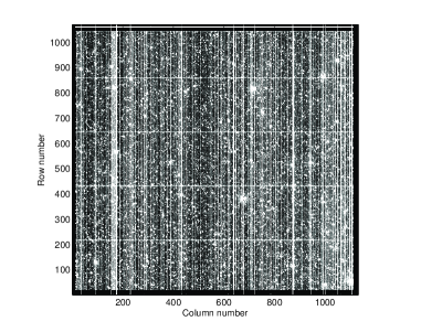
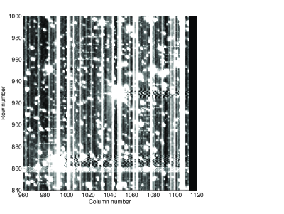
The focal plane consists of 84 separate science readout channels (identified as module#.output#) and four fine guidance sensor (FGS) channels all of which are read out synchronously. Each channel has several regions available to collect calibration, or ‘‘collateral’’ data (Figure 1). There are two sets of columns of virtual pixels: (1) 12 columns of bias-only pixels resulting from 12 leading pixels in the serial register (‘‘leading black’’), and (2) a 20 column serial over-scan region (‘‘trailing black’’). There are also two sets of rows of collateral pixels: (1) the first 20 rows, which are covered by an aluminum mask (‘‘masked smear’’), and (2) a 26 row parallel over-scan region (‘‘virtual smear’’). During science data collection, a coadded sum of specified columns of the trailing black and rows of both the masked and virtual smear are stored at each cadence for each channel.
Since Kepler has no shutter, we cannot take standard dark frames. Instead, the CCDs can be reverse-clocked so that none of the signal from the stars and sky reaches the CCD output, allowing us to measure the bias level throughout the image.
Finally, a full frame image (FFI) mode is available, in which all the pixels in the focal plane are stored. FFIs are invaluable for examining detector properties, verifying pointing, and verifying the target aperture definitions; however, at 380 megabytes each, only a limited number can be processed and stored. Reverse-clocked data and FFIs are taken periodically throughout the mission (Haas et al., 2010).
3. Detector Properties
Each of Kepler’s detector channels has distinct properties important for understanding and analyzing the pixel data, roughly divided into standard CCD detector characteristics and those unique to Kepler’s design. Where possible instrument characterization was performed on the ground (Argabright et al., 2008), though some had to be done during commissioning. A significant portion of commissioning was spent with the dust-cover on, in order to measure characteristics that would later be masked by star light. The latter half of commissioning included measurements of the photometer’s point spread function, pixel response, and focal plane geometry parameters, as discussed in Bryson et al. (2010). Commissioning observations resulted in a series of focal plane models that are used throughout the pipeline processing and are available at the data archive 111http://archive.stsci.edu/kepler/.
3.1. Standard Detector Properties
Because of the large number of photons collected from our typical targets, low read noise is not critical and the focal plane median value of 95 e- read-1, or approximately 1 digital number (DN) per read, is sufficient. The focal plane is maintained at C, reducing dark current effectively to zero. The CCDs are operated to guarantee that the full-well of 1.1 million electrons is not clipped by the 14-bit analog-to-digital converter (ADC) range, resulting in a median gain of 112 electrons DN-1. The high quantum efficiency (QE) back-illuminated CCDs combine with the broad bandpass so that stars with Kepler magnitude saturate depending on the field of view (FOV) location. The observed nonlinearity over the full range of input up to and beyond saturation is on the order of after accounting for charge bleeding.
Since Kepler’s goal is not absolute photometry, an accurate global flat field image is not required, but we do use a local flat, or pixel response non-uniformity (PRNU) map for calibration. The PRNU image maps each pixel’s relative brightness variation from the local mean, expressed in percent (Van Cleve & Caldwell, 2009). The median standard deviation of the pixel values in the PRNU image across the focal plane is . A ‘‘bad pixel’’ map, constructed by thresholding the PRNU map to find outliers, shows that of the FOV is affected by pixel or column defects.
Table 1 summarizes the standard CCD detector properties as measured during ground testing and updated during photometer commissioning.
3.2. Kepler-Specific Instrument Properties
Kepler’s design and operation result in several non-standard properties that influence the content of the raw pixels: readout smear, charge injection, and digital data requantization.
Because there is no shutter, stars shine on the CCDs during readout, resulting in trails along columns that contain stars. Each pixel in a given column of the image ---including the masked and virtual smear rows--- receives the same smear signal (Figure 1). The column-by-column smear level in each image is measured in the smear regions. Smear signals are typically small, since each pixel only ‘‘sees" a star for the readout time (0.52 s) divided by the total number of rows (1070); therefore smear is not a significant contributor to photometric noise.
The science CCDs are operated with an electrical charge injection feature that injects charge at the top of each CCD for four consecutive rows at a signal level approximately 40% of full well. The signal appears entirely in the virtual smear. Charge injection serves the dual purpose of filling radiation induced traps in the CCDs and providing a stable signal for monitoring the readout electronics, or ‘‘local detector electronics’’ (LDE), undershoot artifact (§ 4.1).
In order to store and downlink pixel data for 170,000 targets, the CCD output must be compressed from 23 bits pixel-1 to 4--5 bits pixel-1. Because of the Poisson noise intrinsic in the data, we can afford to requantize (after the initial analog-to-digital conversion) so that the effective noise due to quantization is a constant percentage of the intrinsic noise for all signal levels. For higher signals with more shot noise, more ADC output values are mapped on to a single requantized value. With the step size for a signal with intrinsic variance , the total variance, , is the quadrature sum of the observational noise and the quantization noise:
| (1) |
(Note that the variance of a uniform random variable of unit width is 1/12.) Kepler data are requantized such that the quantization noise is at most 1/4 of the intrinsic noise, , resulting in a total noise increase of . Requantization reduces the number of bits pixel-1 from 23 to 16 and greatly improves compressibility for subsequent lossless steps in the compression process (Haas et al., 2010).
4. Instrument Artifacts
Ground testing uncovered several instrumental artifacts, each of which was investigated to understand the cause, impact, and cost to fix or mitigate. Based on reviews by the Kepler Team and outside experts, the project dispositioned each of these artifacts. There were several for which the Kepler Team and review boards decided that the potential impact to the mission did not warrant the risk of fixing them. These artifacts were extensively characterized on the ground and then again during commissioning. For those with the largest impact, the data processing pipeline either already corrects for them, or corrections are under development (Jenkins et al., 2010b). Table 2 summarizes the FOV potentially affected by each artifact. Values for artifact levels given below are based on 43 days of science data collection.
4.1. LDE Undershoot
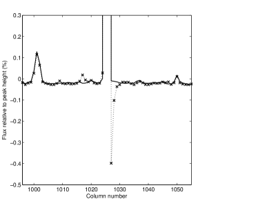
Testing of the LDE signal chain on star-like images revealed a large signal-dependent trailing undershoot in the video. The primary cause was traced to the use of a bipolar-input AD8021 operational amplifier in the correlated double-sample circuit. Corrective action to replace this amplifier with the junction field effect transistor-input AD8065 in all video channels resulted in greatly reducing this artifact, from an initial 2% amplitude and 12 pixels duration to a median amplitude of 0.34% and 3 pixels duration, as measured in flight data (Figure 2). The undershoot distortion can be modeled as an invertible, linear, shift-invariant digital filter, meaning we can correct the pixel values provided we have enough pixels upstream (lower column numbers) of the pixel of interest. To this end, a column of pixels is prepended to each target aperture, and two targets were added to each channel to monitor the undershoot response to both an impulse and a step change. An undershoot correction is included in the pixel calibration pipeline (Jenkins et al., 2010b).
4.2. FGS Clocking Cross Talk
Cross talk from the FGS clocks to the science CCD video signals injects a complex pattern into the bias image of every science channel with an amplitude up to 20 DN read-1 (Argabright et al., 2008). Because the FGS and science CCDs share the same master clock, the pattern is spatially fixed; however, the amplitude of the cross talk is dependent on the temperature of the LDE. The cross talk has three distinct components based on the state of the FGS CCDs as the science pixel is read out (see Figure 1): FGS CCD frame transfer, parallel transfer, and serial transfer (which shows no cross talk). Approximately 20% of targets have at least one of the parallel or frame-transfer cross talk pixels in their aperture. Without mitigation, the cross talk introduces a small time-varying bias into a target’s flux time series as the LDE temperature changes with orbital position.
In order to measure the cross talk thermal dependence, a series of dark FFIs were taken at different temperatures during commissioning. Both the levels and their thermal dependence are consistent with ground characterizations. The signal in each cross talk pixel type can be modeled as an offset from the bias level that is linear in time and LDE board temperature (Van Cleve & Caldwell, 2009). This model removes the cross talk effect to the level of the read noise for all but a few pixel types on the most affected channels. The temporal component decreased significantly during commissioning with a damping time on the order of a week, indicative of a transient effect such as out-gassing. With the dust cover on, the focal plane was warmer during the dark data collection than during science operations, so the model is used to extrapolate the measured cross talk levels to those we see during operations, allowing us to generate a bias image, or ‘‘two dimensional (2D) black’’ for calibration that includes the clocking cross talk.
4.3. 2D Black Artifacts
Ground tests revealed several artifacts associated with the 2D structure of the dark images. Their extent on the focal plane was observed to be small, as was the likelihood that they would worsen or spread. The dark images obtained in flight are completely consistent with ground test results. Nevertheless, the analysis pipeline does not yet include a means of identifying changes in these features, so time series that are released with the current processing version may contain artifact features at signal levels discussed below.
4.3.1 High-frequency Oscillations
A temperature-sensitive amplifier oscillation at 1 GHz was detected in some CCD video channels during the artifact investigation. We suspect that the origin of this oscillation is from the AD8021 operational amplifiers used extensively in the video signal chain, which may show subtle layout-dependent instability when used at low gains. The oscillation’s frequency range, rate of change, and pattern among the channels matched closely those characteristics in the dark images, strongly suggesting that the artifact is a moiré pattern generated by sampling the high-frequency oscillation at the serial pixel clocking rate. Since the characteristic source frequency drifts with time and temperature of the electronic components by as much as , the signal from a given pixel in a series of dark images has a time varying signature. This signature may be highly correlated with neighboring pixels and yet poorly correlated with slightly more distant pixels. When the oscillation frequency is a harmonic of the serial clocking frequency, a DC shift occurs producing a horizontal band offset from the mean bias-level in the image. As the frequency drifts with temperature, the point on the image where this DC shift occurs moves up or down from sample-to-sample, producing a rolling band.
Forty-six of the 84 readout channels have never exhibited this behavior and an additional 9 channels have thus far not exhibited this behavior at a detectable level in flight. Typically, in the remaining 29 channels, of the FOV exhibits the moiré pattern with peak-to-peak amplitudes DN read-1 pixel-1, while another exhibits between and 0.1 DN read-1 pixel-1. Two output channels, 9.2 and 17.2, typically exhibit DN read-1 pixel-1 moiré pattern peak-to-peak amplitudes over their entire fields-of-view. The resulting total FOV fraction typically affected by moiré signal at or above a level of 0.1 DN read-1 pixel-1 (0.02 DN read-1 pixel-1) is 9% (15%). For comparison, 0.1 DN read-1 pixel-1 is the change in signal per pixel in a typical magnitude star aperture for an Earth-size planet transit. We have adopted the conservative threshold of 0.02 DN read-1 pixel-1, or roughly of the per pixel signal from an Earth-size transit, in order to put an upper bound on the potential impact from image artifacts. While the moiré amplitude per pixel in these channels is significant, how the artifact affects our ability to detect small planets depends on its frequency, sum within a target aperture, and variations over time-scales of interest to transit detection. Based on the first 33.5 days of data from science operations, Jenkins et al. (2010a) find the instrument is meeting the 6-hour precision requirement across the focal plane for the quietest 30% of stars. The two worst moiré channels, 9.2 and 17.2, exhibit a 20% increase in 6-hour noise over the focal plane average at magnitude, as measured by the standard deviation of 6-hour binned flux time series. Such an increase is small compared with the factor of 1.5 spread in the distribution of dwarf star precision at magnitude (Jenkins et al., 2010a).
4.3.2 Scene-dependent Artifacts
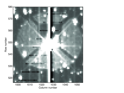
As a consequence of the sensitivity of the oscillating LDE component to temperature, the thermal transient introduced during readout by the signal from a bright star causes additional localized changes in bias-level (Figure 1). These scene dependent artifacts persist over a range of hundreds of pixels in the columns following bright stars. In the 29 output channels exhibiting the moiré pattern, approximately of the FOV may be affected by these artifacts above the 0.02 DN read-1 pixel-1 level.
A second scene dependent effect is observed on all channels. A bright star produces a strong undershoot signal as discussed above, but the undershoot signal extends for hundreds of pixels at a very low level rather than the 20 pixels currently used for the inverse filter. This extended undershoot signal varies in proportion to variations in the source star’s light curve. We estimate that of CCD rows contain stars bright enough to introduce extended undershoot signals which suggests that of pixels are at risk to be affected by this artifact. Of these, we conservatively estimate that are actually affected above the 0.02 DN read-1 pixel-1 level. This means of the total FOV is subject to this effect.
4.3.3 Start-of-line Ringing
A transient signal initiated at the onset of serial clocking of each row is well-modeled as a series of 5 superimposed, slightly under-damped oscillations which extend for roughly 150 pixels. This start-of-line ringing is evident on all output channels, but shows much less thermal sensitivity than the oscillations discussed previously. The initial amplitude of the oscillations is 1 DN read-1 pixel-1; however, the pattern is static, so the current processing algorithms adequately remove the artifact to accuracies 0.02 DN read-1 pixel-1. We do not expect this artifact to impact photometric precision.
5. Summary
We have used commissioning and the first month of science operations to characterize Kepler’s instrument performance. The basic properties of the photometer are unchanged from ground testing. Image artifacts are consistent with ground observations, though star light creates scene dependence of the moiré pattern signal, complicating mitigation plans. Corrections in the current analysis pipeline for static FGS clocking cross talk, LDE undershoot, and start-of-line ringing are found to remove these artifacts to a level sufficient to meet Kepler’s precision requirements. We are currently testing mitigations for the thermally varying FGS cross talk, moiré pattern, and extended undershoot, which will subsequently be implemented in the analysis pipeline. Results indicate that we can reduce the levels of these artifacts to DN read-1 pixel-1 over 80%--90% of the focal plane, with the remainder flagged for use in subsequent analysis steps (Jenkins et al., 2010b). The photometer is currently providing measurements of unprecedented precision and time coverage, giving us great confidence that the Kepler Mission will meet its science goals and make many unexpected discoveries.
References
- Argabright et al. (2008) Argabright, V. S., et al. 2008, Proc. SPIE, 7010, 70102L
- Borucki et al. (2010) Borucki, W. J., et al. 2010, Science, submitted
- Bryson et al. (2010) Bryson, S. T., et al. 2010, ApJ, this issue
- Haas et al. (2010) Haas, M. R., et al. 2010, ApJ, this issue
- Jenkins et al. (2010a) Jenkins, J. M., et al. 2010a, ApJ, this issue
- Jenkins et al. (2010b) ---. 2010b, ApJ, this issue
- Koch et al. (2010) Koch, D. G., et al. 2010, ApJ, this issue
- Van Cleve & Caldwell (2009) Van Cleve, J., & Caldwell, D. A. 2009, Kepler Instrument Handbook, KSCI 19033-001 (Moffett Field, CA: NASA Ames Research Center), http://archive.stsci.edu/kepler/
| Parameter | Where Measured | Minimum | Maximum | Median |
|---|---|---|---|---|
| Read noise (e- read-1) | Flight | 81 | 307 [149]aaFlight measurements of read noise and dark current are contaminated by image artifacts for several of the noisiest channels (§ 4). Values for non-artifact channels are given in square brackets, where different. | 95 |
| Dark current (e- pix-1 s-1) | Flight | -8.1[-3.2]aaFlight measurements of read noise and dark current are contaminated by image artifacts for several of the noisiest channels (§ 4). Values for non-artifact channels are given in square brackets, where different. | 7.5 | 0.25 |
| QE at 600 nm | Ground | 0.81 | 0.92 | 0.87 |
| Gain (e- DN-1) | Ground | 94 | 120 | 112 |
| Saturation (Kepler Mag)bbSaturation range is calculated using the measured QE variations, a vignetting model, and the observed central pixel flux fraction range of 0.28--0.64. | Flight | 11.6 | 10.3 | 11.3 |
| PRNUccPRNU is a measure of local pixel response variation and does not include large-scale optical effects such as vignetting (§ 3.1). (%) | Ground | 0.82 | 1.20 | 0.96 |
| LDE Undershoot (%) | Flight | 0.08 | 1.92 | 0.34 |
Note. — Minimum, maximum, and median are taken across all 84 channels of the focal plane.
| Potential Extent | FOV at Risk | |
|---|---|---|
| Artifact | on FOVaa‘‘Potential extent’’ indicates the fraction of the FOV where the artifact could potentially be seen. ‘‘FOV at risk’’ indicates the fraction where we could see time varying signals at or above 0.02 DN read-1 after existing and planned mitigations in the analysis pipeline. See the text for discussion. (%) | DN/readaa‘‘Potential extent’’ indicates the fraction of the FOV where the artifact could potentially be seen. ‘‘FOV at risk’’ indicates the fraction where we could see time varying signals at or above 0.02 DN read-1 after existing and planned mitigations in the analysis pipeline. See the text for discussion. (%) |
| LDE undershoot | 100 | 0 |
| FGS cross talk | 20 | 0 |
| Moiré pattern | 45 | 15bbThe FOV values do not add since artifacts overlap. Scene dependent moiré pattern drift adds unique FOV and extended undershoot adds . |
| Scene dependent moiré | 45 | 7bbThe FOV values do not add since artifacts overlap. Scene dependent moiré pattern drift adds unique FOV and extended undershoot adds . |
| Extended undershoot | 100 | 10bbThe FOV values do not add since artifacts overlap. Scene dependent moiré pattern drift adds unique FOV and extended undershoot adds . |