Isothermal reentrant effect in a mesoscopic cylindrical structure of a superconductor coated with a normal metal layer

Abstract

The coherent phenomena in mesoscopic cylindrical normal metal (N) - superconductor (S) structures have been investigated theoretically. The magnetic moment (persistent current) of such a structure has been calculated numerically and (approximately) analytically. It is shown that the current in the N-layer corresponding to the free energy minimum is always diamagnetic. As the field increases, the magnetic moment (current) exhibits jumps at certain values of the trapped magnetic flux and the NS structure changes to a state with smaller absolute value of the diamagnetic moment. This occurs when the persistent current is unable to screen the external field. The magnetic moment increase stepwise and the system changes into a new stable state. The magnetic field penetrates into a larger volume of the N-layer. The new state has smaller absolute value of the diamagnetic moment. Experimentally, this is interpreted as the presence of a paramagnetic addition in the system (paramagnetic reentrant effect). The results obtained are in qualitative agreement with the experiments conducted by P. Visani, A. C.Mota, and A. Pollini, Phys. Rev. Lett. 65, 1514 (1990).

I Introduction

The Meissner effect in a mesoscopic cylindrical structure consisting of a superconductor coated with a pure normal-metal layer has interesting features due to the coherent quantum effects in the normal metal. They are observable when there is a good contact between S and N constituents. This problem within the quasiclassical Eilenberger formalism was first investigated theoretically by Zaikin 1a .

Recent advanced technologies of preparation of pure samples have enabled to investigate the coherence properties of mesoscopic samples taking a proper account of the proximity effect 2a . The samples were superconducting Nb wires with a radius $R$ of tens of microns coated with a thin layer $d$ of high-purity Cu, Ag or Au. Mota and co-workers 3a detected surprising behavior of the magnetic susceptibility $\chi$ of a cylindrical NS structure (N and S are for the normal metal and the superconductor, respectively) at very low temperatures ( T $<$ $100$ mK ) in an external magnetic field parallel to the NS boundary. Most intriguingly, a decrease in the sample temperature below a certain point $T_{r}$ (at a fixed field) produced a paramagnetic reentrant effect: the decrease of magnetic susceptibility of the structure is changed to an unexpected grow. A similar behavior was observed in the isothermal reentrant effect in a field decreasing to a certain value $\mathrm{H}_{r}$ below which the susceptibility started to grow sharply. It is emphasized in Ref. 4a that the detected magnetic response of the NS structure is similar to the properties of the persistent currents in mesoscopic normal rings.

There have been numerous attempts to explain the paramagnetic reentrant effect theoretically 5a ; 6a ; 7a . However, the predicted amplitudes of the effect were too small ( except for 6a ) to account for the experimental facts. Fauchere, Belzig and Blatter 6a explain the large paramagnetic effect assuming strong repulsive electron-electron interaction in noble metals. The proximity effect in the N metal induces an order parameter will be shifted by $\pi$ from the order parameter $\Delta$ of the bulk superconductor. This generates the paramagnetic instability of the Andreev states, and the density of states of the NS structure exhibits a single peak near zero energy. The theory developed in Ref. 6a essentially relies on the assumption of the repulsive electron interaction in the normal region.

Maki and Haas 7a made the assumption that in noble metals (Ag, Au) p-wave superconductors may occur with a transition temperature of order $10$ mK. Below $T_{c}$ p -wave triplet superconductivity emerges around the periphery of the cylinder. The diamagnetic current flowing in the periphery is compensated by a quantized paramagnetic current in the opposite direction thus providing a simple explanation for the reentrant effect.

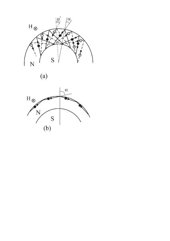
Figure 1: Two classes of trajectories in the normal metal of the NS structure in a magnetic field: trajectories forming the Andreev levels (a): trajectories colliding only with the dielectric boundary (b ). This figure has been taken from 9a .

As in 5a , the authors of 7a also allow for paramagnetic current in the system, which flows in the opposite direction to the diamagnetic current. Its amplitude is sufficient to explain the reentrant effect, but this theory says nothing about the temperature and field dependences of magnetic susceptibility at ultra-low temperatures and in low magnetic fields.

A theoretical basis for understanding the paramagnetic reentrant effect has been proposed in 8a ; 9a ; 10a . The theory is essentially based on the properties of the quantized levels of the NS structure. The Meissner effect is rather special in a superconducting cylinder coated with a pure normal-metal layer. The applied magnetic field generates superconducting current in the surface layer whose thickness is equal to the field penetration depth $\delta$. Simultaneously, the Aharonov-Bohm effect generates persistent current (through the mechanism of the Andreev scattering of quasiparticles) in the normal layer near the NS boundary. If N and S metals are separated by a dielectric layer destroying the Andreev scattering, the additional current disappears, and the Meissner effect returns to its usual form. The levels with energies no more than $\Delta$ (2$\Delta$ is the gap of the superconductor) appear inside the normal metal bounded by the dielectric (vacuum) on one side and the superconductor on the other side. Because of the Aharonov-Bohm effect 11a , the spectrum of the NS structure in a weak field is a function of the magnetic flux. The specific feature of the Andreev quantum levels of the structure is that by varying field $\mathrm{H}$ (or temperature $T$) each level in the well periodically comes into coincidence with the chemical potential of the metal. As a result, the state of the system suffer strong degeneracy, and the density of states on the energy of the NS sample experiences resonance spikes 9a . This contributes significantly to the magnetic moment and causes a reentrant effect. Note that in 9a the calculation was performed for orbital susceptibility. In 6a the explanation involves the spin (Pauli) susceptibility of the system.

In this study we calculated the free energy of the NS structure and its magnetic moment (current of magnetization) in the magnetic field. An approximate analytical calculation was supplemented with a numerical one based on the exact spectrum of Andreev levels 12a in the NS contact. Our approach is not based on application of the Eilenberger equation. We calculate the thermodynamic potential to obtain the magnetic moment.

II Theory and results

II.1 Spectrum of Quasiparticles of the NS Structure

Consider a superconducting cylinder with the radius $R$ which is concentrically embedded with a thin layer $d$ of a pure normal metal. The structure is placed in a magnetic field $\vec{H}\left(0,0,\mathrm{H}\right)$ oriented along the symmetry axis of the structure. It is assumed that the field is weak to the extent that the effect of twisting of quasiparticle trajectories becomes negligible. It actually reduces to the Aharonov-Bohm effect 11a , i.e., allows for the increment in the phase of the wave function of the quasiparticle moving along its trajectory in the vector potential field.

We proceed with a simplified model of NS structure in which the order parameter magnitude changes stepwise at the NS boundary ( $\Delta\left(x\right)=\Theta\left(-x\right)$, $\mathrm{Im}\left(\Delta\right)=0$, a bulk superconductor in the region $x<0$ and a normal metal layer in the region $0\leq x\leq d$ ). It is also assumed that the magnetic field does not penetrate into the superconductor. The coherent properties observed in the pure normal metal can be attributed to its large ”coherence” length $\xi_{N}\left(T\right)=\frac{\hbar\cdot\mathrm{v}_{F}}{\pi\cdot k_{B}T}$ ( $\mathrm{v}_{F}$ is the Fermi velocity, $k_{B}$ is the Boltzmann constant) at very low temperatures ($\xi_{N}\left(T\right)$ $\gg$ $d$). Besides, the spectrum of quasiparticles was obtained assuming a negligible curvature of the NS boundary.

One can easily distinguish two classes of trajectories, inside the normal metal. One of them includes the trajectories which collide in succession with the dielectric and NS boundaries (Fig.1). The quasiparticles moving along these trajectories have energies $\left|E\right|<\Delta$ and are localized inside the potential well bounded by a high dielectric barrier ( $\simeq$ $1eV$ ) on one side and by the superconducting gap $\Delta$ on the other side ($\Delta$ $=$ $3.56\cdot$ $k_{B}T_{c}/2$, $\Delta(\mathrm{Nb})$ $\approx$ $1.42$ meV). On its collisions, the quasiparticle is reflected specularly from the dielectric and experiences the Andreev scattering at the NS boundary 12a . We introduce an angle $\alpha$ at which the quasiparticle hits the dielectric boundary. The angle is measured in the positive direction from the normal to the boundary (Fig.1). In this case the first class contains the trajectories with $\alpha$ varying within the range $-\alpha_{c}\leq\alpha\leq\alpha_{c}$ ( $\alpha_{c}$ is the angle at which the trajectory touches the NS boundary, sin$\left(\alpha_{c}\right)$ $=$ $\frac{R}{R+d}$ ).

Figure 2: The dependence of the density of states of the NS structure on the magnetic flux $\Phi$ ( $E=E_{F}=0$ ). Normalization was performed for the flux $\Phi_{{\small max}}$ corresponding to the highest value of $\nu\left(\Phi\right)$ ($\ \Phi_{max}\approx 2.175$ ).

Another class includes the trajectories whose spectra are formed by collisions with the dielectric only, i.e., the trajectories with $\alpha>\alpha_{c}$. The two groups of trajectories produce significantly different spectra of quasiparticles. The distinctions are particularly obvious in the presence of the magnetic field. The trajectories with $\alpha\lesssim\alpha_{c}$ form a spectrum of Andreev levels which contains an integral of the vector potential field. The spectrum characterizes the magnetic flux through the area of the triangle between the quasiparticle trajectory and the part of the NS boundary. It also determines the magnitude of the screening current produced by ”particles” and ”holes” in the N layer. These states are responsible for the reentrant effect. The trajectories with $\alpha>\alpha_{c}$ do not collide with the NS boundary. The states induced by these trajectories are practically similar to the ”whispering gallery” type of states appearing in the cross section of a solid normal cylinder in a weak magnetic field 13a , 14a . The size of the caustic of these trajectories is of the order of the cylinder radius, i.e., they correspond in high magnetic quantum numbers. The spectrum thus formed carries no information about the parameters of the superconductor, and it is impossible to meet the resonance condition in this case. These states make a paramagnetic contribution in the thermodynamics of the NS structure but their amplitude is small ( $\sim 1/\left(k_{F}\cdot R\right)$ ). It is therefore discarded from further consideration. Our interest will be concentrated on the trajectories with $\left|\alpha\right|\leq\alpha_{c}$.

The spectrum of quasiparticles of the NS structure can be obtained easily using the multidimensional quasiclassical method generalized for the case of the Andreev scattering in the system 15a , 16a . After collision with the NS boundary the ”particle” transforms into a ”hole”. The ”hole” travels practically along the path of the ”particle” but in the reverse direction (Fig.1).

The spectrum was derived by quantizing the adiabatic invariant $\frac{1}{2\pi}\oint\vec{P}\cdot d\vec{s}$ , where $\vec{P}$ $=$ $\vec{p}+$ $\frac{e}{c}\vec{A}$, $\vec{A}$ $=$ $\left(0,A_{y}\left(x\right),0\right)$, $\vec{P}_{0}$ $=$ $\vec{p}_{0}-$ $\frac{\left|e\right|}{c}\vec{A}$ for a ”particle” and $\vec{P}_{1}$ $=$ $\vec{p}_{1}+$ $\frac{\left|e\right|}{c}\vec{A}$ for a ”hole”. Note that each collision with the NS boundary multiplies the wave function amplitude of the quasiparticle by a factor of $\exp\left(-i\arccos\left({E/\Delta}\right)\right)$.

Figure 3: Free energy (normalized per value $\Omega\left(\Phi_{\max}\right)$) as a function of the flux $\Phi$.

Let $\mathrm{{\mathcal{L}}}_{0}$ be the length of the quasiparticle trajectory between the collisions at the boundaries of the N layer. We thus 8a , 9a arrive at the expression for the spectrum of the Andreev levels in the NS structure:

$$E_{n}\left(q,\alpha,\Phi\right)=\frac{\pi\hbar\mathrm{v}_{L}(q)}{\mathrm{{\mathcal{L}}}_{0}}\left[n+\frac{1}{\pi}\arccos\left(\frac{E_{n}\left(q,\alpha,\Phi\right)}{\Delta}\right)-\frac{\tan\left(\alpha\right)}{\pi}\Phi\right].$$ (1)

Here $\mathrm{v}_{L}(q)={\sqrt{p_{F}^{2}-q^{2}}/m^{\ast}}$, $\mathrm{{\mathcal{L}}}_{0}$ is length of the quasiparticle trajectory, $p_{F}$ is the Fermi momentum, $q$ is the quasiparticle momentum component along the cylinder axis ( $\left|q\right|\leq p_{F}$ ), ${m^{\ast}}$ is the effective mass of the quasiparticle, and $\Phi_{0}={hc/2e}$ is the superconducting flux quantum. The factor $\Phi$ appearing in the last term in Eq. (1) has the meaning of ”phase”

$$\Phi=\frac{2\pi}{\Phi_{0}}\int\limits_{0}^{d}A_{y}\left(x\right)dx$$ (2)

which is dependent on the vector potential field $\vec{A}$ $=$ $\left(0,A_{y}\left(x\right),0\right)$. The spectrum of Eq. (1) is similar to Kulik’s spectrum 17a for the current state of the SNS contact. However, Eq. (1) includes an angle-dependent magnetic flux instead of the phase difference of the contacting superconductors.

The length of the quasiparticle trajectory ( $2AB$ ) is readily found from Fig.1 using the sine and cosine theorems:

$$AB=d\cdot\left(\frac{\cos\left(\alpha\right)-\sqrt{\sin\left(\alpha_{c}\right)^{2}-\sin\left(\alpha\right)^{2}}}{1-\sin\left(\alpha_{c}\right)}\right)$$ (3)

where sin$\left(\alpha_{c}\right)$ $=$ $\frac{R}{R+d}$, $-\alpha_{c}\leq\alpha\leq\alpha_{c}$ . The spectrum in Eq. (1) was derived assuming that the mean free path of the quasiparticles was much longer than the cross-section perimeter of the cylinder and the requirement $d\ll R$ was obeyed. In this limit $\mathrm{{\mathcal{L}}}_{0}$ $=$ $2AB$ $\cong$ ${2d/\cos\left(\alpha\right)}$ $\left(\underset{\alpha_{c}\rightarrow\pi/2}{\lim}AB={d/\cos\left(\alpha\right)}\right)$ , i.e., the radius $R$ drops out from the expression for the spectrum. Although the boundary curvature of the sample is disregarded, the information about its cylindrical geometry is retained through a correct choice of the limits of integration for the angle $\alpha$: $-\alpha_{c}\leq\alpha\leq\alpha_{c}$. Putting $\mathrm{{\mathcal{L}}}_{0}$ $=$ ${2d/\cos\left(\alpha\right)}$, we obtain the following expression for the spectrum ( as in 9a ):

$$E_{n}\left(q,\alpha,\Phi\right)=\frac{\pi\hbar\mathrm{v}_{L}(q)\cos\left(\alpha\right)}{2d}\left[n+\frac{1}{\pi}\arccos\left(\frac{E_{n}\left(q,\alpha,\Phi\right)}{\Delta}\right)-\frac{\tan\left(\alpha\right)}{\pi}\Phi\right].$$ (4)

The spectrum in Eq. (4) has an important feature 8a , 9a . As the ”phase” $\Phi$ Eq. (2) changes, the density of states exhibits resonance spikes. Every time when the Andreev level coincides with the chemical potential of the metal, the state of the NS structure suffers strong degeneracy showing up spikes. The dependence of the density of states upon the magnetic flux calculated numerically for the NS system is illustrated in Fig.2.

Note that in 1a , 18a the diamagnetic current of NS structure was calculated using $\alpha_{c}=\pi/2$ instead of the upper limit of integration for the angle ( $\alpha_{c}<\pi/2$ ) and assuming implicitly an infinitely large number of Andreev levels. Therefore, these results cannot be conformed with the experimental findings. The reason is not only that the calculation was made for a flat geometry rather than for a curved NS boundary. Numerical analysis shows that an adequate interpretation of the experimental magnetic moment-field dependence is possible only with a proper choice of the upper limit of integration with respect to $\alpha$. If $\alpha>\alpha_{c}$ or $\alpha_{c}=\pi/2$, the consideration includes effectively the states unrelated to the Andreev levels.

II.2 Self-consistent equation

To calculate the ”phase” $\Phi\left(T,\mathrm{H}\right)$ from Eq. (2), we should know the distribution of the vector potential field inside the normal metal. Zaikin 1a has shown that the proximity effect caused the Meissner effect leads to an inhomogeneous distribution of the vector potential field over the N layer of the structure:

$$A_{y}\left(x\right)=\mu_{0}\mathrm{H}x+\mu_{0}j\cdot x\left(d-{x/2}\right)$$ (5)

where $\mu_{0}$ is the permeability of free space ( the SI system of units is employed, the geometry of the proximity model system is the same as in 19ains Fig 1). This expression can be obtained from the Maxwell equation $rot\left(rot\left(\vec{A}\right)\right)$ $=$ $\mu_{0}\vec{j}$ $=$ $\left(0,\mu_{0}j,0\right)$ assuming that the current density is uniform over the cross-section of the conductor and the boundary condition $\left.\vec{A}\right|_{x=0}$ $=$ $0$, $\left.rot\left(\vec{A}\right)\right|_{x=d}$ $=$ $\vec{B}\left(0,0,\mu_{0}\mathrm{H}\right)$ is met. The fact that the current density is constant in the N-layer follows from spatial homogeneity of the density of Andreev levels over the whole thickness of the N-layer. In cylindrical geometries, if the N-layer thickness is not thin compared to the radius ( $d\gtrsim R$ ), the current density is not constant in space 19a .

The magnetic moment per unit length of the N-layer $M\left(\mathrm{H}\right)=-\frac{1}{\mu_{0}}\frac{d\Omega\left(T,\Phi\left(\mathrm{H}\right)\right)}{d\mathrm{H}}$ ( z-component ) and the current density $\vec{j}$ are related via a relation

$$M\left(T,\mathrm{H}\right)=\frac{1}{2}\int\limits_{V_{N}}\left[\vec{r}\times\vec{j}\left(\vec{r}\right)\right]_{z}dV=\frac{-1}{\mu_{0}}\frac{d\Omega}{d\mathrm{H}}$$ (6)

where $V_{N}$ is a volume of the N-layer unity height, $\Omega\left(T,\Phi\right)$ is the free energy per unit length. Then, the current appears from Eq. (6) is a function of the magnetic flux $\Phi$ and temperature:

$$j=-\frac{1}{\pi R^{2}d\cdot\mu_{0}}\frac{d\Omega\left(T,\Phi\left(\mathrm{H}\right)\right)}{d\mathrm{H}}$$ (7)

We can write down the self-consistent equation for $\Phi\left(T,\mathrm{H}\right)$ using Eqs. (2), (5) and (7):

$$\Phi\left(T,\mathrm{h}\right)=\mathrm{h}+\eta\cdot M^{\ast}\left(\Phi\right)\frac{\partial\Phi\left(T,\mathrm{h}\right)}{\partial\mathrm{h}}$$ (8)

where $\mathrm{h}=\frac{\mathrm{H}}{\mathrm{H}_{0}}$, $\mathrm{H}_{0}=\frac{\Phi_{0}}{\pi d^{2}\cdot\mu_{0}}$, $\eta=\frac{d^{2}}{3R^{2}\Phi_{0}\mathrm{H}_{0}}$, $M^{\ast}\left(\Phi\right)=-\frac{d\Omega}{d\Phi}$ 20FNT . To describe the field effect on the magnetic moment

$$M\left(T,\mathrm{H}\right)=\frac{M^{\ast}\left(T,\Phi\right)}{\mu_{0}\mathrm{H}_{0}}\cdot\frac{\partial\Phi\left(T,\mathrm{h}\right)}{\partial\mathrm{h}}$$ (9)

of a NS structure, it is necessary to find the dependence $\Phi\left(T,\mathrm{h}\right)$ from Eq. (8). After calculating the free energy $\Omega\left(T,\Phi\right)$ from the spectrum of Eq. (4), we can estimate the magnetic moment Eq. (9) using a solution of the differential equation (8): $M\left(T,\mathrm{H}\right)$ $=$ $\frac{1}{\eta\cdot\mu_{0}\mathrm{H}_{0}}$ $\left(\Phi\left(T,\mathrm{h}\right)-\mathrm{h}\right)$. In this article, we used the ”thermodynamic” approach Eq. (7) which leads to the first order differential equation (8) for the function $\Phi\left(T,\mathrm{h}\right)$.

Figure 4: The magnitude of $M^{\ast}\left(\Phi\right)/\left|M^{\ast}\left(\Phi_{\max}\right)\right|$ as a function of the flux $\Phi$.

However, another approach based on of the Eilenberger formalism ( 1a , 18a ) yields an algebraic self-consistent equation ( Eq. 22 in (18a ) ) for the ”phase” $\Phi\left(T,\mathrm{h}\right)$:

$$\Phi\left(T,\mathrm{h}\right)=\mathrm{h}+const\cdot j\left(\Phi\right)$$ (10)

( in notation Eq., (8) ). In this equation the function $j\left(\Phi\right)$ is described by the expression Eq., 13 in 1a . Clearly, both approaches (8), (10) will lead to quite different dependencies of $M\left(T,\mathrm{H}\right)$ on magnetic field and temperature. In our point of view, the self-consistent equation (10) cannot be applied to the cylindrical NS structures. While deriving the expression for a current 1a , the author assumed that $\alpha_{c}=\pi/2$ (the case of a plane). This means account for the contribution non-Andreev states ( $\alpha>\alpha_{c}$). For the calculation of thermodynamic potential in equation (8) we shall use the actual magnitude of the parameter $\alpha_{c}$ ( $sin(\alpha_{c})=R/(R+d)$ ). The approximation $d<<R$ was used by us in the derivation of the spectrum (4) only. In other words, the neglect of the curvature of cylindrical samples (i.e. the path length of quasiparticles was choosen as ${d/\cos\left(\alpha\right)}$ (3)) does not entail the need of account for the states with $\alpha>\alpha_{c}$ for the cylindrical NS of structures (Fig.1).

II.3 Analytical estimation of the magnetic moment of the NS structure

We proceed from the expression for the free energy of a NS contact:

$$\Omega=-k_{B}T\sum\limits_{n,q,\alpha,s}\ln\left(1+e^{-\frac{E_{n}\left(q,\alpha\right)}{k_{B}T}}\right)$$ (11)

where the summation is over the spin variable $s=\pm 1$ and all the states related to the quasiparticles trajectories with $\left|\alpha\right|\leq\alpha_{c}$ in Eq. (4). Then, we obtain the following expression for the free energy per unit length $L$

$$\Omega\left(\Phi\right)=-\frac{R\cdot k_{B}T}{\pi\hbar^{2}}\sum\limits_{n=-\infty}^{n=\infty}\int_{-\alpha c}^{\alpha_{c}}\int_{-p_{F}}^{p_{F}}\ln\left(1+\exp\left(-\frac{E_{n}\left(q,\alpha,\Phi\right)}{k_{B}T}\right)\right)\sqrt{p_{F}^{2}-q^{2}}\cos\left(\alpha\right)dqd\alpha$$ (12)

where the energy $E_{n}\left(q,\alpha,\Phi\right)$ is given by the exact expression for the spectrum in Eq. (4). For simplification, we introduce the dimensionless quantities $\varepsilon_{n}=\frac{E_{n}\left(q,\alpha,\Phi\right)}{\Delta}$, $\sigma=\frac{\hbar\cdot p_{F}}{2d\cdot\Delta\cdot m^{\ast}}$, $-1\leq\varepsilon_{n}\leq 1$, ( $\Delta$ is the superconducting gap ) and perform the change of variables $\left\{q,\alpha\right\}\rightarrow\left\{u,v\right\}$:

$$\left\{\begin{array}[]{c}u={\sigma\cdot\sqrt{1-\left(\frac{q}{p_{F}}\right)^{2}}\cdot\cos\left(\alpha\right)}\\ v={\sigma\cdot\sqrt{1-\left(\frac{q}{p_{F}}\right)^{2}}\cdot\sin\left(\alpha\right)}\end{array}\right..$$ (13)

The spectrum and the free energy become

$$\varepsilon_{n}=\left[n\pi+\arccos\left(\varepsilon_{n}\right)\right]\cdot u-\Phi\cdot v\text{,}$$ (14)

$$\Omega\left(\Phi\right)=c_{1}T\sum\limits_{n=0}^{n=\infty}\iint\limits_{S}\frac{u\ln\left(2\cosh\left(\frac{\varepsilon_{n}}{2c_{2}T}\right)\right)dudv}{\sqrt{\sigma^{2}-u^{2}-v^{2}}}$$ (15)

where $c_{1}=-2\frac{R\cdot\Delta\cdot c_{2}}{\pi}\cdot\left(\frac{p_{F}}{\sigma\cdot\hbar}\right)^{2}$, $c_{2}=\frac{k_{B}}{\Delta}$, $0\leq u\leq\sigma$, $-\sigma\sin\left(\alpha_{c}\right)\leq v\leq\sigma\sin\left(\alpha_{c}\right)$, $\varepsilon_{n}\overset{def}{=}\varepsilon_{n}\left(u,v,\Phi\right)$, an integration domain $S$ is a sector of a circle of radius $\sigma$. In the expression (15) we also took into account the symmetry of the spectrum in Eq. (14):

$$\varepsilon_{-\left|n\right|}\left(u,v,\Phi\right)=-\varepsilon_{\left|n\right|-1}\left(u,-v,\Phi\right)\text{.}$$ (16)

Making use of the relation

$$\frac{d\varepsilon_{n}}{d\Phi}=-\frac{v\cdot\sqrt{1-\varepsilon_{n}^{2}}}{u+\sqrt{1-\varepsilon_{n}^{2}}}$$ (17)

we evaluate the derivative of the free energy with respect to the flux $M^{\ast}\left(\Phi\right)=-\frac{d\Omega}{d\Phi}$:

$$M^{\ast}\left(\Phi\right)=c_{3}\sum\limits_{n=0}^{n=\infty}\iint\limits_{S}\frac{uv\tanh\left(\frac{\varepsilon_{n}}{2c_{2}\cdot T}\right)\sqrt{1-\varepsilon_{n}^{2}}dudv}{\left(u+\sqrt{1-\varepsilon_{n}^{2}}\right)\sqrt{\sigma^{2}-u^{2}-v^{2}}}$$ (18)

where $c_{3}=\frac{R\cdot\Delta}{\pi}\left(\frac{p_{F}}{\sigma\cdot\hbar}\right)^{2}$. Eqs. (9), (8) and (18) fully determine the non-linear magnetic response of a cylindrical NS structure to an externally applied magnetic field $\mathrm{H}$.

The integral expression of Eq. (18) suggests that $M^{\ast}\left(\Phi\right)$ is the odd function of the flux $\Phi$: $M^{\ast}\left(\Phi\right)$ $=$ $-M^{\ast}\left(-\Phi\right)$. A linear term of the function $M^{\ast}\left(\Phi\right)$ has been determined from an approximate estimation of the integral in Eq. (18). This calculation is similar to that in the Attachment of 9a . The final expression for the magnetic moment is

$$M\left(T,\mathrm{h}\right)\simeq M_{0}\sum\limits_{n=0}^{n_{0}}\frac{\ln\cosh\left(\frac{T_{A}\cdot\tilde{n}}{2T}\right)}{\tilde{n}^{3}\left[1+\left(\frac{\Phi\left(T,\mathrm{h}\right)}{\pi\cdot\tilde{n}}\right)^{2}\right]^{\frac{{3}}{2}}}$$ (19)

where $\tilde{n}$ $=$ $n+\frac{1}{2}$, $T_{A}$ $=$ $\frac{\hbar\cdot\mathrm{v}_{F}}{2\pi d\cdot k_{B}}$ is Andreev temperature, $M_{0}=$ $-$ $c_{3}$ $\cdot$ $\sigma^{2}\cdot\left(\frac{T}{T_{A}}\right)$ $\cdot$ $\Phi\left(T,\mathrm{h}\right)\cdot\frac{\partial\Phi\left(T,\mathrm{h}\right)}{\partial\mathrm{h}}$, the ”phase” $\Phi\left(T,\mathrm{h}\right)$ is a solution of the differential equation (8), $n_{0}$ is the number of Andreev levels in the potential well ( $n_{0}\approx\frac{\Phi\left(T,\mathrm{h}\right)}{\pi}\tan\left(\alpha_{c}\right)$ ). Eq. (19) shows that the magnetic moment is diamagnetic in the range of small fields ( $\Phi\left(\mathrm{h}\right)=const\cdot\mathrm{h}$, $const>0$ ) and allows for the contributions of ”particles” and ”holes”.

II.4 Numerical results

Let us compare two approaches described above for the calculation of the magnetic moment of the NS structure. Fig.5 shows the function $M^{\ast}\left(\Phi\right)$ and dependency of the current on the magnetic flux obtained in the Green’s function approach. For comparison, we obtained the dependence $M^{\ast}\left(\Phi\right)$ at the same value $\alpha_{c}=\pi/2$ as was used in the derivation of the formula $j\left(\Phi\right)$ in 18a . In the initial part (linear in the $\Phi$) both curves coincide. In this approximation ($\Phi\left(\mathrm{h}\right)=const\cdot\mathrm{h}$) the self-consistent equation (9) turns into Eq. (10). Thus, at small values of the magnetic field we would obtain the same field dependence of the magnetic moment $M\left(T,\mathrm{h}\right)$ for the NS structure in both approaches.

Figure 5: The magnitudes $M^{\ast}\left(\Phi\right)/\left|M^{\ast}\left(0.1\right)\right|$ and $j\left(\Phi\right)/\left|j\left(0.1\right)\right|$ as the functions of the flux $\Phi$ (for explanation see text).

However, in large fields the behavior $M\left(T,\mathrm{h}\right)$ is quite different. To calculate $M\left(T,\mathrm{h}\right)$ from Eq. (9), we have used the following physical values of the NS structure: $R=8.3$ $\mu$m, $d=3.2$ $\mu$m, ($\alpha_{c}=36^{0}$), $\mathrm{v}_{F}\left(\text{Au}\right)=1.4\cdot 10^{8}$ cm/s, $\Delta\left(\text{Nb}\right)=1.42$ meV ( $\sigma=0.644$, $\eta\cdot c_{3}=5.3\cdot 10^{3}$, $\mathrm{H}_{0}=51$A/m $=0.64$ Oe ). The selected parameters are close to those used in the experiment 3a ; 4a ; 20a .

The results of calculation according to formulas (15) and (18) are illustrated in Fig. 3, 4. While plotting Fig. 3, the nonzero quantity $\Omega\left(\Phi=0\right)$ was omitted. The dependence $M^{\ast}\left(\Phi\right)=-\frac{d\Omega}{d\Phi}$ (Fig. 4) crosses the abscissa thereby determining singular points of the differential equation (8). The dependence $\Phi\left(\mathrm{h},\mathrm{T}\right)$ calculated through numerical solution of the self-consistency equation (8) exhibits jumps and is illustrated in Fig.6a for the branches corresponding to the minimum of the Gibbs free energy Gibbs :

$$\mathcal{G}\left(T,\mathrm{H}\right)=\Omega\left(T,\mathrm{H}\right)+\frac{1}{2\mu_{0}}\int\limits_{V_{N}}\left(\vec{B}-\mu_{0}\vec{H}\right)^{2}dV$$ (20)

where $\vec{B}=rot\left(\vec{A}\right)$, $\vec{H}=\vec{H}\left(0,0,\mathrm{H}\right)$. The magnetic moment $M\left(\mathrm{h}\right)$ and the free energy $\Omega\left(\mathrm{h}\right)$ as functions of the magnetic field are shown in Fig. 7a, Fig. 6b. Each jump $\Delta\Omega$ of the free energy (see Fig. 6b) is accompanied by the jump of the magnetic moment $\Delta M$ (see Fig. 7a) in such a way that the Gibbs free energy (20) is a continuous function of versus the magnetic field $\mathrm{h}$. We have not performed an analysis of behavior Gibbs free energy (20) near the points where the magnetic moment has jumps because it is beyond the semi-classical approximation adopted in this article.

III Conclusions

The goal of our study was to interpret the experiments performed by A. C. Mota et al., 3a ; 4a , who detected an anomalous behavior of the magnetic susceptibility of the NS structure in a weak magnetic field at millikelvin temperatures.

Figure 6: a) the dependence of $\Phi\left(T,\mathrm{h}\right)$ on the magnetic field $\mathrm{h}$. b) the relative free energy $\Omega\left(\mathrm{h}\right)/\Omega\left(\mathrm{h}_{\max}\right)$ ($\Phi\left(\mathrm{h}_{\max}\right)=\Phi_{\max}$) as a function of the magnetic field $\mathrm{h}$.

Previously 8a ; 9a , the anomalous behavior of the NS structure was attributed to the properties of the quantized Andreev levels depending on the magnetic flux that varies with the temperature and magnetic field. We used the ”thermodynamic” approach for the calculation of the magnetic moment of normal region of NS structure. Within the framework of the self-consistent equation (8), we have managed to trace the role of the parameter $\alpha_{c}$ in thermodynamics of NS of structures (Fig. 4 and Fig. 5). Failure connected with the use of the quasi-classical Green-function technique 1a for the explanation of the experimental data (Mota et al) is a consequence of account for states which are non-Andreev ones ( $\alpha>\alpha_{c}$ ) for the cylindrical NS structures. Geometrically, this can be seen from figure Fig. 1. The quasiparticle trajectories ( $\alpha>\alpha_{c}$ ) hitting the dielectric boundary only are responsible for the paramagnetic current of a small amplitude ( $\sim 1/(k_{F}\cdot R)$) (we neglected this current).

The proximity effect is crucial for the reentrant effect. The amplitude of the resonance spikes in the density of states strongly depends on the probability of the Andreev reflection at the NS boundary. It is therefore assumed that the normal metal and the superconductor are in a good electric contact. The spectrum Eq. (4) was obtained by the method of multidimensional quasi-classical approach 15a ; 16a .

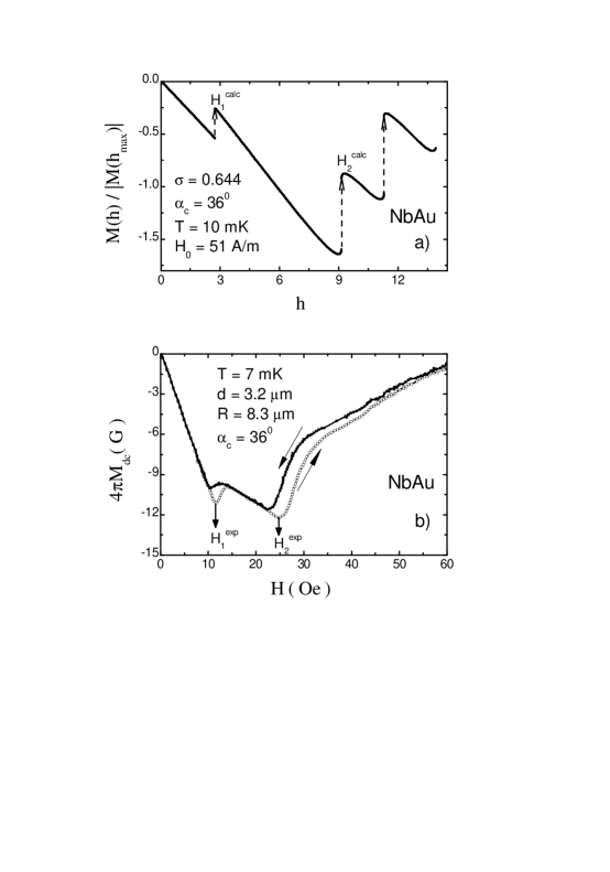
Figure 7: a) The magnetic moment of the NS structure versus the magnetic field $\mathrm{h}$. b) Isothermal dc-magnetization curve at $T=7$ mK for the sample 41AuNb 20a . Used by courtesy of A. C. Mota.

In doing so, we assumed (i) the condition of smallness of N-layer thickness in comparison with the radius of the cylindrical superconductor, (ii) the validity of the model of a stepwise-varing order parameter of the structure, (iii) the independence of $\Delta$ on the magnetic field. This permitted us to pass over from the curved NS boundary to a flat one. The information about the cylindrical geometry of the sample was retained because the critical angle at which a quasiparticle hits the dielectric boundary $\alpha$ is smaller than $\alpha_{c}$. The problem was further simplified by assuming that the reflected quasiparticle performed a reciprocating motion, i.e., a ”particle” and a ”hole” pass along the same trajectory but in opposite direction. Actually, here there exists a lot of quasi reciprocating trajectories with the energies near $\varepsilon\sim 0$. These trajectories lead to the spikes in the density of states and were taken into account for numerical computation. The numerical calculation shows that the nonlinearity of flux $\Phi\left(\mathrm{T},\mathrm{h}\right)-$ field dependence ( $\mathrm{T=}$ constant ) (Fig.6a) gives rise to quite interesting features of $M\left(T,\mathrm{H}\right)$. The magnetic moment in the N layer appears to be always diamagnetic. The paramagnetic contribution to current (the paramagnetic reentrant effect) was not detected. However, we have obtained the stepwise change in absolute value of the magnetic moment with increasing magnetic field (Fig.7a). This behavior can be interpreted as an appearance in the magnetic moment the paramagnetic additives. A behaviour of the NS structure changes from one stable state to another and the magnetic field penetrates further into a bulk of the N layer. The new state has smaller absolute value of the diamagnetic moment, which is interpreted experimentally as an evidence of a paramagnetic addition in the system (Fig.7b). When the field grows further, $\left|M\left(\mathrm{H}\right)\right|$ increases again until its new value makes the system to jump to a next stable state with a smaller absolute value of the diamagnetic moment, and the magnetic field penetrates deeper inside the normal metal (Fig.7a). The number of the moment jumps depends on the number of Andreev levels in the NS structure. Under the isothermal condition, the values of the magnetic field at which jumps occur, do not coincide when the magnetic field changes from small to larger values and in the opposite direction because of a special dependence of the Gibbs free energy on the field. This sort of hysteresis was observed experimentally in 4a ; 20a (Fig.7b).

Numerical comparison between data presented at Fig.7b and Fig.7a shows that $M\left(T,\mathrm{H}\right)$ (Fig. 7a) gives the qualitative description of the experimental data which obey the scaling rule: $\mathrm{H}_{2}^{\exp}/\mathrm{H}_{1}^{\exp}\simeq\mathrm{H}_{2}^{calc}/\mathrm{H}_{1}^{calc}\simeq 5/2$. For the quantitative description of the temperature and magnetic field dependence of the magnetic moment NS of structures, it will be important to take into account the exact spectrum of Andreev levels, the latter is supposedly possible within the framework of the Bogoliubov – de Gennes equations only.

Note that our consideration was entirely based on the model of free electrons without account of strong electron-electron repulsion.

IV Acknowledgement

The authors thank A. N. Omelyanchouk, I. O. Kulik, I. V. Krive and G. I. Japaridze for useful discussions.

References

- (1) A. D. Zaikin, Solid State Comm. 41, 533 (1982).
- (2) A. C. Mota, P. Visani, and A. Pollini, J. Low Temp. Phys. 76, 465 (1989).
- (3) P. Visani, A. C. Mota, and A. Pollini, Phys. Rev. Lett. 65, 1514 (1990).
- (4) A. C. Mota, P. Visani, A. Pollini, and K. Aupke. Physica B 197, 95 (1994).
- (5) C. Bruder, and Y. Imry, Phys. Rev. Lett. 80, 5782 (1998).
- (6) A. L. Fauchere, W. Belzig, and G. Blatter, Phys. Rev. Lett. 82, 3336 (1999).
- (7) K. Maki and S. Haas, Physica C 341-348, 2667 (2000).
- (8) G. A. Gogadze, Fiz. Nizk. Temp. 31,120 (2005) [Low Temp. Phys. 31, 94 (2005)].
- (9) G. A. Gogadze, Fiz. Nizk. Temp. 32, 716 (2006) [Low Temp. Phys. 32, 546 (2006)].
- (10) G. A. Gogadze, Fiz. Nizk. Temp. 34, 225 (2008) [Low Temp. Phys. 34, 173 (2008)].
- (11) Y. Aharonov and D. Bohm, Phys. Rev. 115, 485 (1959).
- (12) A. F. Andreev, Zh. Eksp. Teor. Fiz. 46,1823 (1964) [Sov. Phys. JETP 9, 1228 (1964)]
- (13) E. N. Bogachek and G. A. Gogadze, Zh. Eksp. Teor. Fiz. 63, 1839 (1972) [Sov.Phys.JETP 36, 973 (1973)]
- (14) N. B. Brandt, E.N. Bogachek, N. D. Gitsu, G.A. Gogadze, I. O. Kulik, A. A. Nikolaeva, and Ya. G. Ponomarev, Fiz. Nizk. Temp. 8, 718 (1982) [Sov. J. Low Temp. Phys. 8, 358 (1982)]
- (15) J. B. Keller and S.I. Rubinow, Ann. Phys ( N. Y. ) 9, 24 (1960)
- (16) G. A. Gogadze, R. I. Shekhter, and M. Jonson, Fiz. Nizk. Temp. 27, 1237 (2001) [Low Temp. Phys. 27, 913 (2001)].
- (17) I. O. Kulik, Zh. Eksp. Teor. Fiz. 57, 1745 (1969) [Sov. Phys. JETP 30, 944 (1969)]
- (18) A. V. Galaktionov and A. D. Zaikin, Phys. Rev. B 67,184518 (2003).
- (19) W. Belzig, C. Bruder and A. L. Fauchère, Phys. Rev. B 58, 14531 (1998).
- (20) W. Belzig, C. Bruder, and G. Schon, Phys. Rev. B 53, 5727 (1996).
- (21) G. A. Gogadze S. N. Dolya, Fiz. Nizk. Temp. 35, 932 (2009).
- (22) F. B. Müller-Allinger, A. C. Mota, Phys. Rev. B 62, 6120 (2000).
- (23) A. L. Fauchère G. Blatter, Phys. Rev. B 56, 14102 (1997).