Computing the Maximum Slope Invariant in Tubular Groups

Abstract

We show that the maximum slope invariant for tubular groups is easy to calculate, and give an example of two tubular groups that are distinguishable by their maximum slopes but not by edge pattern considerations or isoperimetric function.

1 Introduction

The main examples of tubular groups are constructed from $\mathbb{Z}^{2}$ by amalgamating along cyclic subgroups.

Tubular groups have been used as examples of various phenomena. Brady and Bridson computed isoperimetric functions for the groups

$$BB(p,r)=\left<a,b,x,y\mid[a,b]=1,\,x^{-1}a^{p}x=a^{r}b,\,y^{-1}a^{p}y=a^{r}b^{-1}\right>$$

with $0<p<r$ and found that the degrees of the isoperimetric functions form a dense set in $[2,\infty)$. The Dehn function of $BB(p,r)$ is $x^{n}$ with $n=2\log_{2}\frac{2r}{p}$ [1].

Later Brady, Bridson, Forester and Shankar, [2], used more complicated examples of tubular groups, called “snowflake groups”, to show that all the rationals in that interval appear.

Other examples include the examples of Croke and Kleiner [4] and Wise’s group [7].

There are two quasi-isometry invariants readily available among these groups. For the Brady-Bridson and snowflake groups we have the isoperimetric exponent. Mosher, Sageev and Whyte give another: the collection of affine equivalence classes of edge patterns [5].

In a previous paper [3] we gave an algorithm to decide whether or not two tubular groups are quasi-isometric. In the course of the proof we constructed a tree, the “tree of P–sets”, related to the Bass-Serre tree of a particular graph of groups decomposition of the group. The (directed) edges of this tree come with a parameter, the “height change across the edge”. The maximum slope invariant for the tubular group is then the maximum coarse slope of any ray in the tree, where coarse slope is average height change per unit length, in an appropriate sense. It follows from the quasi-isometry algorithm that the maximum coarse slope is a quasi-isometry invariant of the group (at least in certain cases).

Among the groups $BB(p,r)$ the edge patterns are all equivalent and it turns out that the isoperimetric exponent is a complete quasi-isometry invariant. One might wonder whether the equivalence classes of edge patterns and the isoperimetric exponent always determine the quasi-isometry class of a tubular group.

The answer is “no”. In this note we give an example of two tubular groups with the same equivalence classes of edge patterns and the same isoperimetric exponent but different maximum slopes.

The method of computing the maximum slopes is easy and generalizes to many classes of tubular groups. Dehn functions for tubular groups are known only for special cases, and running the quasi-isometry algorithm of [3] is laborious, so, in practice, checking that maximum slopes are equal is a good test to perform before running the quasi-isometry algorithm.

2 Preliminaries

In this section we recall the necessary terminology and facts about tubular groups and quasi-isometries of tubular groups.

We simplify the exposition considerably by considering only tubular groups that are graphs of groups with vertex groups $\mathbb{Z}^{2}$ and edge groups $\mathbb{Z}$ such that the edge groups incident to a vertex inject into exactly three distinct maximal cyclic subgroups.

The reader is referred to [3] for more background in tubular groups and graphs of groups, and for proofs of claims in this section.

2.1 The Geometric Model

Consider a graph of groups with vertex groups $\mathbb{Z}^{2}$ and edge groups $\mathbb{Z}$ such that the edge groups incident to a vertex inject into exactly three distinct maximal cyclic subgroups. A model for such a group can be built by taking a torus for each vertex, an annulus for each edge, and gluing a boundary of an annulus to a torus according to the corresponding edge injection.

If we then choose a metric on each torus and annulus and lift to the universal cover we get a geodesic metric space quasi-isometric to the group, which we call the geometric model.

Consider one of the vertex $\operatorname{\mathbb{Z}}^{2}$ groups. Suppose $\operatorname{\mathbb{Z}}^{2}=\left<a,b\mid[a,b]=1\right>$. The “usual” metric is the one for which the word $a^{x}b^{y}$ in $\mathbb{Z}^{2}$ corresponds to the point with Cartesian coordinates $(x,y)$ in the standard Euclidean plane. Suppose the incident edge groups inject into the maximal cyclic subgroups containing $a$, $a^{r}b^{s}$, and $a^{t}b^{u}$, where $0$, $\frac{s}{r}$ and $\frac{u}{t}$ are distinct. This can be arranged by picking a new generating set, if necessary, since we have assumed that there are three distinct maximal cyclic subgroups.

This means that with this choice of coordinates, in the universal cover the edge spaces incident to this vertex space attach along lines of slope $0$, $\frac{s}{r}$ and $\frac{u}{t}$. For any of these slopes, since the edge group $\mathbb{Z}$ is infinite index in the vertex group $\mathbb{Z}^{2}$, in the universal cover we have infinitely many edge spaces gluing on to the vertex space along lines of the same slope.

We will have three different infinite families of parallel lines in the plane. This collection of families of infinite lines is called the edge pattern in the vertex space.

From work of Mosher, Sageev and Whyte [5] we know that a quasi-isometry of tubular groups takes vertex groups to within bounded distance of vertex groups. We also know that these edge patterns are the coarse intersection patterns of the various vertex spaces, and must be preserved up to bounded error by quasi-isometries. Furthermore, when there are infinite families of at least three different slopes in a plane, then only quasi-isometries of the plane that preserve the three families are bounded distance from an affine map. Therefore, the affine equivalence class of the set of slopes in a vertex space is a quasi-isometry invariant of the group.

For our examples we may assume that any quasi-isometry restricts on each vertex space to an affine map that takes three specified slopes to three specified slopes. Projectively there is a unique map that does this, so the only freedom in the map is translation and rescaling the entire plane by a constant. Moreover, there is a convenient choice of metric that will make quasi-isometries on the vertex spaces particularly nice.

Choose the metric on the vertex group so that the word $a^{x}b^{y}$ corresponds to the vector $A(_{y}^{x})$ in the plane, where $A$ is the matrix:

$$A=\left(\begin{matrix}1&-\frac{1}{2}\frac{ru+st}{su}\\ 0&\frac{\sqrt{3}}{2}\frac{ru-st}{su}\end{matrix}\right)$$

This is a convenient choice because it makes the line pattern symmetric, the three families of parallel lines differ from one another by angle $\frac{\pi}{3}$. Any permutation of the slopes can be achieved by an isometry of the plane.

Once the metrics have been chosen on the vertex groups we can define height change across an edge. Each edge group is $\mathbb{Z}$. Define the stretch factor across the (directed) edge to be the ratio of the lengths of the image of the generator of the edge group in the two adjacent vertex groups. The height change across the edge is $-\log_{2}(\text{stretch factor})$.

2.2 Quasi-isometries preserve height change

For $i=1,2$, let $G_{i}$ be a tubular group, $D_{i}$ its Bass-Serre tree, and $X_{i}$ its geometric model. Let $q_{i}\colon\thinspace X_{i}\to D_{i}$ be the usual quotient map. A quasi-isometry $\phi\colon\thinspace X_{1}\to X_{2}$ induces a bijection $\phi_{*}$ from vertices of $D_{1}$ to vertices of $D_{2}$. This bijection of vertices can be extended to a continuous map $D_{1}\to D_{2}$ by connecting the dots.

The height change between two vertices of the Bass-Serre tree of a tubular group is the sum of the height changes across the edges of the geodesic segment joining the vertices.

The quasi-isometry $\phi$ is coarsely height preserving in the sense that there is some constant $C$ so that for any two vertices $v,v^{\prime}\in D_{1}$, the height change between $\phi_{*}(v)$ and $\phi_{*}(v^{\prime})$ is within $C$ of the height change between $v$ and $v^{\prime}$.

2.3 Coarse Slope

Let $c\colon\thinspace[0,\infty)\to D_{1}$ be a geodesic ray. A quasi-isometry $\phi\colon\thinspace X_{1}\to X_{2}$ induces a bijection $\phi_{*}$ from vertices of $D_{1}$ to vertices of $D_{2}$, but does not necessarily preserve adjacency. Thus, the ray $\phi_{*}\circ c\colon\thinspace[0,\infty)\to D_{2}$ may not be a geodesic ray.

Let $e$ and $e^{\prime}$ be edges incident to a vertex $v$ in $D_{i}$. We say that $e$ and $e^{\prime}$ are parallel at $v$ if $q_{i}^{-1}(e)\cap q_{i}^{-1}(v)$ and $q_{i}^{-1}(e^{\prime})\cap q_{i}^{-1}(v)$ are parallel lines in $q_{i}^{-1}(v)$. Equivalently, $e$ and $e^{\prime}$ are parallel at $v$ if their stabilizer subgroups in $G_{i}$ are contained in a common maximal cyclic subgroup of the stabilizer of $v$.

We say that $c$ has a twist at $t$ (or at $v=c(t)$) if the incoming and outgoing edges at $c(t)$ are not parallel at $c(t)$.

Quasi-isometries preserve twists: $c$ has a twist at $t$ if and only if $\phi_{*}\circ c$ has a twist at $t$.

So, while the length of a segment in $D_{1}$ is not preserved by $\phi_{*}$, the number of twists along that segment is, and we define the coarse slope of a ray $c$ in $D_{1}$ to be the ratio of height change to number of twists.

Let $\mathrm{Twist}_{c}(t)$ denote the number of twists of $c(0,t)$. A ray $c$ in $D_{i}$ has coarse slope $m$, $\operatorname{slope}(c)=m$, if there exists a $C>0$ such that for all $t$,

$$m\cdot\mathrm{Twist}_{c}(t)-C\leq h(c(0),c(t))\leq m\cdot\mathrm{Twist}_{c}(t)+C$$

Not every ray has a coarse slope, but $c$ has coarse slope $m$ if and only if $\phi_{*}\circ c$ does. The maximum slope invariant of a tubular group is the quasi-isometry invariant given by the largest number $m$ (possibly $\infty$) that occurs as the coarse slope of a ray in the Bass-Serre tree. (The supremum of coarse slopes is always achieved because the group acts cocompactly on the Bass-Serre tree.)

3 The Procedure

In this section we give the procedure for computing the maximum slope, using the group $BB(p,r)$ to illustrate.

Step 1: Compute the Height Changes:
Start with a graph of groups decomposition. Call the vertices $v_{1},\dots v_{j}$. Choose the metric that makes the edge patterns symmetric and compute height changes across each edge.

$\operatorname{\mathbb{Z}}^{2}$ at 61 780 $a^{p}$ at 53 800 $a^{p}$ at 69 800 $a^{r}b$ at 53 757.8 $a^{r}b^{-1}$ at 69 758

Figure 1: graph of groups for $BB(p,r)$

The graph of groups for $BB(p,r)$ is depicted in Figure 1. Let $x$ and $y$ be stable letters corresponding to the loop on the left and right, respectively. The labels at the ends of the edges indicate that these elements of the vertex group are conjugate by the stable letter associated to the edge, thus $x$ conjugates $a^{p}$ to $a^{r}b$. The fundamental group of the graph of groups is:

$$BB(p,r)=\left<a,b,x,y\mid[a,b]=1,\,x^{-1}a^{p}x=a^{r}b,\,y^{-1}a^{p}y=a^{r}b^{-1}\right>$$

The matrix $A$ that determines the symmetric metric on the vertex group is:

$$A=\left(\begin{matrix}1&0\\ 0&r\sqrt{3}\end{matrix}\right)$$

The height change across $x$ is

$$H=-\log_{2}\frac{|A(^{r}_{1})|}{|A(^{p}_{0})|}=-\log_{2}\frac{2r}{p}$$

The height change across $y$ is also $H$. Note that $H$ is negative since $r>p$.

Step 2: Identify Parallel Edges:
At each vertex, join edges with an arc if their groups inject into a common maximal cyclic subgroup. This happens exactly when the edges are parallel at the vertex.

If there is a loop in the graph such that for every edge-vertex-edge sequence in the loop the two edge groups are parallel and such that the net height change around the loop is not zero, stop. The maximum slope is infinite.

$H$ at 15 781 $H$ at 105 781

Figure 2: height change and parallel edges for $BB(p,r)$

In $BB(p,r)$ the two edge groups both map into the maximal cyclic subgroup $\left<a\right>$ at the top of Figure 2. There are no non-trivial loops for which all edge-vertex-edge transitions involve parallel edges.

Step 3: Fold Parallel Edges:
Subdivide each edge by adding a vertex at the midpoint. Call these new vertices $m_{1},\dots m_{k}$.

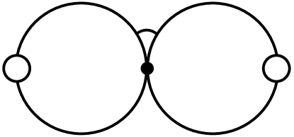
Figure 3: subdivided edges for $BB(p,r)$

At each $v_{i}$, for each collection of edges incident to the vertex and joined by arcs, fold them together by identifying them up to their midpoints.

In the resulting graph of P–sets, label each edge with a height change in such a way that the height changes between the original vertices is preserved. This is always possible. One way to accomplish this is to look at each remaining $m_{i}$. It is adjacent to some of the original vertices $v_{i_{1}},\dots,v_{i_{l}}$. Among these there is some $\alpha$ so that for all $\beta$, the height change from $v_{i_{\alpha}}$ to $v_{i_{\beta}}$ is non-negative. Give the edge from $v_{i_{\alpha}}$ to $m_{i}$ height change 0, and give the edge from $m_{i}$ to $v_{i_{\beta}}$ the height change equal to the height change from $v_{i_{\alpha}}$ to $v_{i_{\beta}}$.

One may check that this graph of P–sets is the quotient by the group action on the tree of P–sets constructed in [3].

We will leave edges with height change 0 unlabeled and undirected.

$|H|$ at 68 800

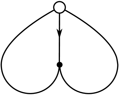
Figure 4: graph of P–sets for $BB(p,r)$

Step 4: Find the Embedded Loop of Maximum Slope:
The effect of this procedure is to collapse parallel edges at a vertex to a single edge. Since we assumed that for each vertex there are exactly three maximal cyclic subgroups containing the edge injections, the original (small black) vertices all have valence 3. The new (large white) vertices represent collections of parallel edges.

Let $c$ be a path in the graph of P–sets and let $v$ be an original vertex in the interior of the path. For any lift $\tilde{c}$ of $c$ to the Bass-Serre tree, $\tilde{c}$ has a twist at the vertex $\tilde{v}$ corresponding to $v$. This means that length of a path in the graph of P–sets corresponds to number of twists in any lift of the path, so we can compute slopes by taking the ratio of height change to length of paths in the graph. (Here we consider edges in the graph to have length one half.)

If the graph of P–sets is a tree then the maximum slope is 0. Otherwise, the maximum slope can be realized by an embedded loop. To see this, consider a loop that is not embedded and has non-zero slope. It contains some embedded sub-loops, and the slope of the entire loop is less than or equal to the maximum of the slopes of the embedded sub-loops.

For $BB(p,r)$ the maximum slope is $|H|=\log_{2}\frac{2r}{p}$. Recall that the isoperimetric exponent for $BB(p,r)$ is $2\log_{2}\frac{2r}{p}$, which is exactly twice the maximum slope.

4 An Example

Consider the snowflake group, $G=G_{r,P}$ of [2], with $P=(4)$, $p=4$, $q=1$. Let $r=2^{p}=16$. This snowflake group has Dehn function $x^{4}$.

$G$ is the fundamental group of a graph of groups with three $\mathbb{Z}^{2}$ vertex groups $\mathbb{Z}^{2}=\left<a_{i},b_{i}\mid[a_{i},b_{i}]=1\right>$ for $i=1,2,3$.

Each vertex has edges injecting into the cyclic subgroups generated by $a_{i}$, $b_{i}$, and $a_{i}b_{i}$.

Figure 5 gives a graph of groups diagram for this group. In the diagram, $a_{4}=b_{3}$ and $c=a_{1}b_{1}=a_{1}a_{2}a_{3}a_{4}$.

$\operatorname{\mathbb{Z}}^{2}$ at 66 731 $\operatorname{\mathbb{Z}}^{2}$ at 106 731 $\operatorname{\mathbb{Z}}^{2}$ at 146 731 $c$ at 55 725 $b_{1}$ at 76 725 $a_{2}b_{2}$ at 92 725 $b_{2}$ at 115 725 $a_{3}b_{3}$ at 131 725 $a_{4}^{16}$ at 157 725 $a_{1}^{16}$ [l] at 66 740 $a_{2}^{16}$ [l] at 106 740 $a_{3}^{16}$ [l] at 146 740

Figure 5: A graph of groups diagram for the snowflake group $G_{16,(4)}$

Conveniently, symmetrization in this case does not stretch the lines, so stretch factors are just ratios of indices. The edge that goes from $a_{i}^{16}$ to $c$ therefore has stretch factor $\frac{1}{16}$, and height change $-\log_{2}\frac{1}{16}=4$. The other edges have 0 height change.

In Figure 6 we have height changes and parallel edges for $G_{16,(4)}$.

4 [l] at 63 746 4 [b] at 75 757 4 [b] at 75 776 4 [b] at 75 790

Figure 6: Height changes and parallel edges for the snowflake group $G_{16,(4)}$

Now if we fold this graph down to a graph of P–sets, Figure 7, we quickly see that the maximum slope in the tree of P–sets for this group is 4 (the smallest loop in the figure realizes the maximum slope). The isoperimetric exponent was also 4.

$4$ at 52 726

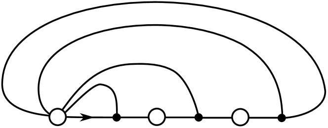
Figure 7: The P–set graph for $G_{16,(4)}$

However, recall that $BB(p,r)$ has isoperimetric exponent equal to twice the maximum slope. $BB(1,2)$ has Dehn function $x^{4}$ but a maximum slope of 2. It is not quasi-isometric to the snowflake group.

5 Generaliztion

The procedure described in Section 3 generalizes to arbitrary tubular groups, subject to constraints described in [3]. First, coarse slope is only well defined when the edge patterns in every vertex space have at least three distinct families of parallel lines. Second, the slopes depend on the choice of symmetric metric on the vertex spaces. For vertex spaces whose edge patterns consist of three or four slopes there is a unique choice, up to isometry and rescaling. For an edge pattern with five or more families of parallel lines this is not always true, there may or may not be a unique choice of symmetric metric. The maximum coarse slope is still useful in distinguishing groups when there are edge patterns without a canonical choice of symmetric metric, but one must take care to identify each pattern in an equivalence class with the same symmetric pattern.

References

- [1] N. Brady and M. R. Bridson, There is only one gap in the isoperimetric spectrum, Geom. Funct. Anal. 10 (2000), no. 5, 1053–1070.
- [2] Noel Brady, Martin R. Bridson, Max Forester, and Krishnan Shankar, Snowflake groups, Perron-Frobenius eigenvalues, and isoperimetric spectra, Geom. Topol. 13 (2009), no. 1, arXiv:math.GR/0608155.
- [3] Christopher H. Cashen, Quasi-isometries between tubular groups, Groups, Geometry and Dynamics, to appear, arXiv:0707.1502.
- [4] Christopher B. Croke and Bruce Kleiner, Spaces with nonpositive curvature and their ideal boundaries, Topology 39 (2000), 549–556.
- [5] Lee Mosher, Michah Sageev, and Kevin Whyte, Quasi-actions on trees II: Finite depth Bass-Serre trees, Mem. Amer. Math. Soc., to appear, arXiv:math.GR/0405237.
- [6] Jean-Pierre Serre, Trees, Springer Monographs in Mathematics, Springer, Berlin, 2003, corrected second printing of the first English edition.
- [7] Daniel T. Wise, A non-hopfian automatic group, Journal of Algebra 180 (1996), no. 3, 845–847.