Classification of the Entangled States $2\times M\times N$

Abstract

We extend the matrix decomposition method(MDM) in classifying the $2\times N\times N$ truly entangled states to $2\times M\times N$ system under the condition of stochastic local operations and classical communication. It is found that the MDM is quite practical and convenient in operation for the asymmetrical tripartite states, and an explicit example of the classification of $2\times 6\times 7$ quantum system is presented.

1 Introduction

Entanglement is an essential feature of quantum theory, describing a quantum correlation that exhibits nonlocal properties. In the seminal work [1], Einstein, Podolsky, and Rosen (EPR) demonstrated through a Gedanken experiment that the quantum mechanics (QM) can not provide a complete description of the “physical reality” for two spatially separated but quantum mechanically correlated particles state which is now known as entangled state. The subsequent Bell theorem manifest the nonlocal character of the quantum correlation in the violation of Bell’s inequalities [2]. As the quantum information science develops, the impact of entanglement goes far beyond the testing of the conceptual foundations of QM. Entanglement is now of central importance in the quantum information theory (QIT) and is thought as the key physical resource to realize quantum information tasks, such as quantum cryptography [3, 4], superdense coding [5, 6], and quantum computation [7], etc. This necessitates the qualitative and quantitative description of the entanglement [8]. However due to the lack of suitable tools for characterizing the entanglement, very limited quantum state space was explored in the quantum information theory.

In quantum information processing (QIP), two states are suited to implement the same task if they can be mutually converted by stochastic local operations and classical communication (SLOCC) [9], and therefore they are said to be in the same equivalent class. For three qubits, known result is that there are two kinds of true tripartite entanglement classes for pure state, namely, GHZ and W states [9]. As the dimensions of each party increases nontrivial aspect shows up, i.e., non-local parameters may resides in the entangled states of $2\times N\times N$ system when $N\geq 4$ [10, 11]. Many investigations concerned the classifications of $2\times M\times N$ states has been done in [10, 12, 13]. In the Refs.[10, 12], an iterated method was introduced to determine all the inequivalent classes of the entangled states of $2\times M\times N$ system based on the “range criterion”, where the entanglement classification of the low dimension system is a prerequisite for the high dimensions ones. Practical classifications of dimensions up to $2\times 4\times 4$ and the related systems of $2\times(M+4)\times(2M+4)$ were given in [10]. With the increasing of dimensions, the complexity of the method grows dramatically because of the iterated nature of their inequivalent proof of the entanglement classes. In a recent work [11] a novel method of classifying the pure state of $2\times N\times N$ systems was introduced in which all the inequivalent true tripartite entanglement classes can be determined directly by using merely the elementary operations on the cubic grid form of the state.

The present work deals with the more general case: quantum state of $2\times M\times N$ systems (pure state if not specified). We show that the method we introduced in [11] can be generalized to the classification of true entangled states of $2\times M\times N$ systems. Although the main tools are the same for $2\times M\times N$ with that of $2\times N\times N$, the generalization is nontrivial and the method for $2\times M\times N$ can help the general classification of $L\times M\times N$ systems. All the inequivalent classes can be generated directly and no followed-up inequivalence proof of these classes is needed. The content goes as follows, in section 2, by representing the $2\times M\times N$ state in the form of matrix pairs, the $2\times M\times N$ states are divided into inequivalent sets under SLOCC. The detailed classification procedures with these inequivalent sets are presented in section 3 and a concrete example of classification of $2\times 6\times 7$ system is given. Finally, in section 4 we give some concluding remarks.

2 Matrix pair representation of $2\times M\times N$ state

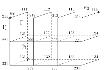
Figure 1: The cubic form for $2\times 3\times 4$ state. The node in the grid labeled $ijk$ represents the matrix elements $\Gamma_{\{i,j,k\}}$.

Adopt the conventions of [11], an arbitrary state of $2\times M\times N$ can be written as

$$|\Psi_{2\times M\times N}\rangle=\sum_{i,j,k}\Gamma_{\{i,j,k\}}\,|i\rangle_{\psi_{0}}|j\rangle_{\psi_{1}}|k\rangle_{\psi_{2}}\;,$$ (1)

where, $\psi_{0}$ represents the first qubit, $\psi_{1}$ and $\psi_{2}$ has the dimension of $M$ and $N$ separately; $\Gamma_{\{1,j,k\}}$ and $\Gamma_{\{2,j,k\}}$ are $M\times N$ complex matrices (we assume $M\leq N$ without loss of generalities). Then the state can be written in the following compact form

$$|\Psi_{2\times M\times N}\rangle=\begin{pmatrix}\Gamma_{\!1}\\ \Gamma_{\!2}\\ \end{pmatrix}.$$ (2)

Clearly, to every state of $2\times M\times N$, there is a form of Eq.(2) that corresponds to it, and a pictorial description of the state is straightforward, see Fig.(1).

The reduced density matrix of state $\Psi_{2\times M\times N}$ is defined as $\rho_{\psi_{i}}=\mathrm{Tr}_{\neg\,\psi_{i}}[|\Psi\rangle\langle\Psi|]$, where $i\in\{0,1,2\}$. For three-partite systems, true (or genuine [9]) entanglement means that reduced density matrices of each partite have full ranks. Let $r$ denote the rank of matrix hereafter, then $r(\rho_{\psi_{0}})=2,r(\rho_{\psi_{1}})=M,r(\rho_{\psi_{2}})=N$ for the true entangled state of $2\times M\times N$ systems. The density matrix in the form of the matrix pairs can be expressed as

$$\rho_{\psi_{0},\psi_{1},\psi_{2}}=(\Gamma_{i})_{jk}(\Gamma_{i^{\prime}})_{j^{\prime}k^{\prime}}^{*}\;,$$ (3)

where $i,i^{\prime}=1,2;j,j^{\prime}=1,2,\cdots,M;k,k^{\prime}=1,2,\cdots,N$. The reduced density matrix (take $\psi_{2}$ as an example) then is

$$\rho_{\psi_{2}} = \mathrm{Tr}_{\psi_{0},\psi_{1}}(\rho_{\psi_{0},\psi_{1},\psi_{2}})$$ (4)

$$= \sum_{ij}(\Gamma_{i})^{*}_{jk^{\prime}}(\Gamma_{i})_{jk}$$

$$= \sum_{i}\Gamma_{i}^{\dagger}\Gamma_{i}\;.$$

Lemma 2.1

$\forall$ $i\in\{0,1,2\}$, $\mathrm{Det}(\rho_{\psi_{i}})=0$, if and only if the cubic form of the three-partite state (see Fig.(1)) can be transformed into a form where at least one plane perpendicular to axis $\psi_{i}$ are zero planes (plane with all its coefficients are zeroes) via ILOs.

The proof is presented in Appendix A. Thus if $\mathrm{Det}(\rho_{\psi_{i}})=0,i\in\{0,1,2\}$, the entanglement of $2\times M\times N$ system reduces to the case of $2\times M^{\prime}\times N^{\prime}$ with $M^{\prime}<M$ or/and $N^{\prime}<N$ which should in principle be considered as an entanglement system of $2\times M^{\prime}\times N^{\prime}$.

3 Classification of $2\times M\times N$ State

Two $2\times M\times N$ states $\widetilde{\Psi}$ and $\Psi$ are said to be SLOCC equivalent if they are connected via invertible local operators (ILOs). That is, $\widetilde{\Psi}$ is SLOCC equivalent to $\Psi$ if

$$|\widetilde{\Psi}_{2\times M\times N}\rangle=T\otimes P\otimes Q\,|\Psi_{2\times M\times N}\rangle\;,$$ (5)

where $T,P,Q$ are invertible complex matrices of dimension $2\times 2$, $M\times M$, and $N\times N$ which act on $\psi_{0}$, $\psi_{1}$, $\psi_{2}$, respectively. Neglecting the extra factor of the determinant of matrices, $T$, $P$, and $Q$ correspond to the special linear groups of $SL(2,\mathbb{C}),SL(M,\mathbb{C}),SL(N,\mathbb{C})$ [9]. Takes the wave function $|\Psi_{2\times M\times N}\rangle$ in the matrix pair form [i.e., Eq.(2)], the ILO operators $T$, $P$, $Q$ in Eq.(5) take the following form

$$|\widetilde{\Psi}_{2\times M\times N}\rangle = \begin{pmatrix}t_{11}&t_{12}\\ t_{21}&t_{22}\end{pmatrix}\begin{pmatrix}P\Gamma_{\!1}Q\\ P\Gamma_{\!2}Q\end{pmatrix},$$ (6)

where $t_{ij}$ are matrix elements of $T$. From Eq.(2) and Eq.(6) we can see that the SLOCC equivalence of the quantum state turns to the connectivity of the matrix pairs $(\Gamma_{\!1},\Gamma_{\!2})$ under the special linear transformations $T,P,Q$. Define the set that contains all the matrices pair $(\Gamma_{\!1},\Gamma_{\!2})$ as $C$. The whole space of $C$ can be partitioned into numbers of subsets with different $n$, $l$

$$C_{n,\;l}=\{(\Gamma_{\!1},\Gamma_{\!2})|\;r_{\mathrm{max}}(\alpha_{1}\Gamma_{\!1}+\beta_{1}\Gamma_{\!2})=n,r_{\mathrm{min}}(\alpha_{2}\Gamma_{\!1}+\beta_{2}\Gamma_{\!2})=l\}\;,$$ (7)

where $r_{\rm max}$ and $r_{\rm min}$ represent the the maximum and minimum rank of the matrices respectively; $\alpha_{i},\beta_{i}\in\mathbb{C}$ and $|\alpha_{i}|+|\beta_{i}|\neq 0$; $l\in[0,n]$, $n\in[0,M]$.

Proposition 3.1

If $(\Gamma_{1},\Gamma_{2})\in C_{n,l}$ and $\exists$ $T,P,Q\in\mathrm{ILO}$, $\begin{pmatrix}\Gamma^{\prime}_{1}\\ \Gamma^{\prime}_{2}\end{pmatrix}=\begin{pmatrix}t_{11}&t_{12}\\ t_{21}&t_{22}\\ \end{pmatrix}\begin{pmatrix}P\Gamma_{1}Q\\ P\Gamma_{2}Q\end{pmatrix}$, then $(\Gamma^{\prime}_{1},\Gamma^{\prime}_{2})\in C_{n,l}$.

(see Appendix B). This proposition implies that the matrix pairs in subsets $C_{n,l}$ with different $n$ or $l$ are SLOCC inequivalent.

3.1 Classification on sets $C_{n,l}$ with $n=M$

We start our classification of $C_{n,\,l}$ in $2\times M\times N$ system from the case $n=M$. Our aim is to construct the subsets $c_{M,l}\subset C_{n,\,l}$ which: (i), it includes representative states of all the inequivalent entanglement classes; (ii), each inequivalent class has only one representative state in $c_{M,l}$.

Because $\forall$ $(\Gamma_{\!1},\Gamma_{\!2})\in C_{M,\,l}$, $\exists$ $T\in\mathrm{ILO}$ (see Appendix B)

$$T\left\lgroup\begin{array}[]{c}\Gamma_{\!1}\\ \Gamma_{\!2}\\ \end{array}\right\rgroup=\left\lgroup\begin{array}[]{cc}t_{11}&t_{12}\\ t_{21}&t_{22}\\ \end{array}\right\rgroup\left\lgroup\begin{array}[]{c}\Gamma_{\!1}\\ \Gamma_{\!2}\\ \end{array}\right\rgroup,$$ (14)

that makes $r(t_{11}\Gamma_{\!1}+t_{12}\Gamma_{\!2})=M$, $r(t_{21}\Gamma_{\!1}+t_{22}\Gamma_{\!2})=l$, so we assume that all the matrix pairs in $C_{M,l}$ have been performed this kind of ILO transformation $T$. That is $r(\Gamma_{\!1})=M$ and $r(\Gamma_{\!2})=l$. Two specific ILOs $P$ and $Q$ can transform $(\Gamma_{\!1},\Gamma_{\!2})$ into the following form

$$\left(\begin{array}[]{l}\Gamma_{\!1}\\ \Gamma_{\!2}\end{array}\right)\xrightarrow{P,Q}\left(\begin{array}[]{ll}\left(\begin{array}[]{ll}E_{\scriptstyle M\times M}&\mathbf{0}_{\scriptstyle M\times(N-M)}\end{array}\right)\\ \left(\begin{array}[]{ll}A_{\scriptstyle M\times M}&B_{\scriptstyle M\times(N-M)}\end{array}\right)\end{array}\right)\;,$$ (21)

where $E$ is an unit submatrix of $P\Gamma_{\!1}Q$, $\mathbf{0}$ is zero submatrix; $A$ and $B$ are submatrix of $P\Gamma_{2}Q$, and all of them have the subscripts as their dimensions. We can represent the submatrix $B_{M\times(N-M)}$ by matrix theory conventions, i.e., $B_{M\times(N-M)}=\Gamma_{2}(\{1,\cdots,M\},\{M+1,\cdots,N\})$.

If $(N-M)>M$, then $r_{\text{max}}(B_{M\times(N-M)})=M$, the right hand of Eq.(21) can be further transformed by ILOs into

$$\left(\begin{array}[]{c}\Gamma_{\!1}\\ \Gamma_{\!2}\end{array}\right)\xrightarrow{P,Q}\left(\begin{array}[]{l}\left(\begin{array}[]{lll}E_{\scriptstyle M\times M}&\mathbf{0}_{\scriptstyle M\times(N-2M)}&\mathbf{0}_{\scriptstyle M\times M}\end{array}\right)\\ \left(\begin{array}[]{lll}\mathbf{0}_{\scriptstyle M\times M}&\mathbf{0}_{\scriptstyle M\times(N-2M)}&E_{\scriptstyle M\times M}\end{array}\right)\end{array}\right)\;,$$ (28)

In the form of the cubic grid (Fig.(1)), this corresponds to that at least $(N-2M)$ vertical planes in the middle of the cube are zero planes, which is actually an entangled states of $2\times M\times 2M$ according to lemma 2.1. Thus here we consider the case $M\geq N/2$.

For arbitrary matrix pair with the form of the right hand of Eq.(21), we implement the following transformation via ILOs

$$\left(\begin{array}[]{ll}\left(\begin{array}[]{ll}E_{\scriptstyle m\times m}&\mathbf{0}_{\scriptstyle m\times(n-m)}\end{array}\right)\\ \left(\begin{array}[]{ll}A_{\scriptstyle m\times m}&B_{\scriptstyle m\times(n-m)}\end{array}\right)\end{array}\right)\xrightarrow{\text{step {\bf i}}}\left(\begin{array}[]{l}\left(\begin{array}[]{lll}E_{\scriptstyle 1A^{\prime}}&\mathbf{0}_{\scriptstyle 1B^{\prime}}&\mathbf{0}_{\scriptstyle 1a}\\ \mathbf{0}_{\scriptstyle 1b}&E_{\scriptstyle 1^{\prime}}&\mathbf{0}_{\scriptstyle 1E^{\prime}}\end{array}\right)\\ \left(\begin{array}[]{lll}A^{\prime}&B^{\prime}&\mathbf{0}_{\scriptstyle 2a}\\ \mathbf{0}_{\scriptstyle 2b}&\mathbf{0}_{\scriptstyle 2c}&E^{\prime}\end{array}\right)\end{array}\right)\;,$$ (39)

where the lower-right submatrix of the right hand side $\Gamma_{\!2}(\{m-r(B)+1,\cdots,m\},\{m+1,\cdots,n\})=E^{\prime}$ has $r(E^{\prime})=r(B)$; $A^{\prime}$, $E_{\scriptstyle 1A^{\prime}}$ are square submatrices with the dimensions $(m-r(E^{\prime}))\times(m-r(E^{\prime}))$; the rest of the matrices are partitioned accordingly, i.e., $\mathbf{0}_{\scriptstyle 1B^{\prime}}$, $B^{\prime}$ have the dimension $(m-r(E^{\prime}))\times r(E^{\prime})$, $\mathbf{0}_{1a}$, $\mathbf{0}_{2a}$ have the dimension of $(m-r(E^{\prime}))\times(n-m)$, $\mathbf{0}_{\scriptstyle 1b}$, $\mathbf{0}_{2b}$ have the dimension $r(E^{\prime})\times(m-r(E^{\prime}))$, $E_{\scriptstyle 1^{\prime}}$, $\mathbf{0}_{\scriptstyle 2c}$ have the dimension $r(E^{\prime})\times r(E^{\prime})$. After the transformation, $\Gamma_{\!1}=(E_{\scriptstyle M\times M},\mathbf{0}_{\scriptstyle M\times(N-M)})$ being unchanged, $\Gamma_{\!2}$ becomes a quasidiagonal matrix and we named this procedure step i.

Next we repartitioned the matrices on the left hand side of Eq.(39) as follows

$$\left(\begin{array}[]{l}\left(\begin{array}[]{lll}E_{\scriptstyle 1A^{\prime}}&\mathbf{0}_{\scriptstyle 1B^{\prime}}&\mathbf{0}_{\scriptstyle 1a}\\ \mathbf{0}_{\scriptstyle 1b}&E_{\scriptstyle 1^{\prime}}&\mathbf{0}_{\scriptstyle 1E^{\prime}}\end{array}\right)\\ \left(\begin{array}[]{lll}A^{\prime}&B^{\prime}&\mathbf{0}_{\scriptstyle 2a}\\ \mathbf{0}_{\scriptstyle 2b}&\mathbf{0}_{\scriptstyle 2c}&E^{\prime}\end{array}\right)\end{array}\right)\xrightarrow{\text{step {\bf ii}}}\left(\begin{array}[]{l}\left(\begin{array}[]{ll|l}E_{\scriptstyle 1A^{\prime}}&\mathbf{0}_{\scriptstyle 1a}&\mathbf{0}_{\scriptstyle 1b}\\ \hline\cr\mathbf{0}_{\scriptstyle 1c}&E_{\scriptstyle 1^{\prime}}&\mathbf{0}_{\scriptstyle 1d}\end{array}\right)\\ \left(\begin{array}[]{ll|l}A^{\prime}&B^{\prime}&\mathbf{0}_{\scriptstyle 2a}\\ \hline\cr\mathbf{0}_{\scriptstyle 2b}&\mathbf{0}_{\scriptstyle 2c}&E^{\prime}\end{array}\right)\end{array}\right)\;.$$ (52)

This is named as step ii. Consider the submatrix $B^{\prime}$, if it is not identically zero we can perform the transformation of step i on the left-top submatrices $\begin{pmatrix}A^{\prime}&B^{\prime}\end{pmatrix}$ of Eq.(52)

$$\left(\begin{array}[]{ll}\left(\begin{array}[]{ll}E_{\scriptstyle 1A^{\prime}}&\mathbf{0}_{\scriptstyle 1a}\end{array}\right)\\ \left(\begin{array}[]{ll}A^{\prime}&B^{\prime}\end{array}\right)\end{array}\right)\xrightarrow{\text{step {\bf i}}}\left(\begin{array}[]{l}\left(\begin{array}[]{lll}E_{\scriptstyle 1A^{\prime\prime}}&\mathbf{0}_{\scriptstyle 1B^{\prime\prime}}&\mathbf{0}_{\scriptstyle 1a^{\prime}}\\ \mathbf{0}_{\scriptstyle 1b^{\prime}}&E_{\scriptstyle 1^{\prime\prime}}&\mathbf{0}_{\scriptstyle 1E^{\prime\prime}}\end{array}\right)\\ \left(\begin{array}[]{lll}A^{\prime\prime}&B^{\prime\prime}&\mathbf{0}_{\scriptstyle 2a}\\ \mathbf{0}_{\scriptstyle 2b^{\prime}}&\mathbf{0}_{\scriptstyle 2c^{\prime}}&E^{\prime\prime}\end{array}\right)\end{array}\right)\;.$$ (63)

This procedure can be done repeatedly (suppose repeat $n$ times), until the $r(B^{(n)})=0$. We can get that the matrix pair $(\Gamma_{\!1},\Gamma_{\!2})$ can be transformed into the following form

$$\Gamma_{\!1}\rightarrow\left(\begin{array}[]{l|lllll}E_{\scriptstyle 1A^{(n)}}&\mathbf{0}&\mathbf{0}&\cdots&\mathbf{0}&\mathbf{0}\\ \hline\cr\mathbf{0}&E_{1^{(n-1)}}&\mathbf{0}&\cdots&\mathbf{0}&\mathbf{0}\\ \vdots&\vdots&\vdots&\ddots&\vdots&\vdots\\ \mathbf{0}&\mathbf{0}&\mathbf{0}&\cdots&\mathbf{0}&\mathbf{0}\\ \mathbf{0}&\mathbf{0}&\mathbf{0}&\cdots&E_{1^{\prime}}&\mathbf{0}\end{array}\right) \equiv \left(\begin{array}[]{ll}E&\mathbf{0}\\ \mathbf{0}&E_{1}\end{array}\right)\;,$$ (71)

$$\Gamma_{\!2}\rightarrow\left(\begin{array}[]{l|lllll}A^{\scriptstyle(n)}&B^{\scriptstyle(n)}=\mathbf{0}&\mathbf{0}&\cdots&\mathbf{0}&\mathbf{0}\\ \hline\cr\mathbf{0}&\mathbf{0}&E^{\scriptstyle(n-1)}&\cdots&\mathbf{0}&\mathbf{0}\\ \vdots&\vdots&\vdots&\ddots&\vdots&\vdots\\ \mathbf{0}&\mathbf{0}&\mathbf{0}&\cdots&E^{\prime\prime}&\mathbf{0}\\ \mathbf{0}&\mathbf{0}&\mathbf{0}&\cdots&\mathbf{0}&E^{\prime}\end{array}\right)\equiv\left(\begin{array}[]{ll}SJS^{-1}&\mathbf{0}\\ \mathbf{0}&E_{2}\end{array}\right)\;,$$ (79)

where the transformed $\Gamma_{\!1}$ is just $(E_{\scriptstyle M\times M},\mathbf{0}_{M\times(N-M)})$, and $E_{1,2}$ are lower-right submatrices defined according to the partition lines; $J$ is the Jordan form of $A^{(n)}$.

As a concrete example here we show how this whole procedure is proceeded on the sets of $C_{4,l}$ of $2\times 4\times 6$ state. The transformation of Eq.(39) is start with

$$\left(\begin{array}[]{ll}\left(\begin{array}[]{ll}E_{\scriptstyle 4\times 4}&\mathbf{0}_{\scriptstyle 4\times 2}\end{array}\right)\\ \left(\begin{array}[]{ll}A_{\scriptstyle 4\times 4}&B_{\scriptstyle 4\times 2}\end{array}\right)\end{array}\right)\xrightarrow{\text{step {\bf i}}}\left(\begin{array}[]{l}\left(\begin{array}[]{lll}E_{\scriptstyle 1A^{\prime}}&\mathbf{0}_{\scriptstyle 1B^{\prime}}&\mathbf{0}_{\scriptstyle 1a}\\ \mathbf{0}_{\scriptstyle 1b}&E_{\scriptstyle 1^{\prime}}&\mathbf{0}_{\scriptstyle 1c}\end{array}\right)\\ \left(\begin{array}[]{lll}A^{\prime}&B^{\prime}&\mathbf{0}_{\scriptstyle 2a}\\ \mathbf{0}_{\scriptstyle 2b}&\mathbf{0}_{\scriptstyle 2c}&E^{\prime}\end{array}\right)\end{array}\right)\;,$$ (90)

where

$$\left(\begin{array}[]{l}\left(\begin{array}[]{lll}E_{\scriptstyle 1A^{\prime}}&\mathbf{0}_{\scriptstyle 1B^{\prime}}&\mathbf{0}_{\scriptstyle 1a}\\ \mathbf{0}_{\scriptstyle 1b}&E_{\scriptstyle 1^{\prime}}&\mathbf{0}_{\scriptstyle 1c}\end{array}\right)\\ \left(\begin{array}[]{lll}A^{\prime}&B^{\prime}&\mathbf{0}_{\scriptstyle 2a}\\ \mathbf{0}_{\scriptstyle 2b}&\mathbf{0}_{\scriptstyle 2c}&E^{\prime}\end{array}\right)\end{array}\right)=\left(\begin{array}[]{l}\left(\begin{array}[]{ll|ll|ll}1&0&0&0&0&0\\ 0&1&0&0&0&0\\ \hline\cr 0&0&1&0&0&0\\ 0&0&0&1&0&0\end{array}\right)\\ \left(\begin{array}[]{ll|ll|ll}\times&\times&+&+&0&0\\ \times&\times&+&+&0&0\\ \hline\cr 0&0&0&0&1&0\\ 0&0&0&0&0&1\end{array}\right)\end{array}\right)\;.$$ (107)

Here, the rank of $B_{\scriptstyle 4\times 2}$ must be 2, otherwise the state will not be a true entangled state of $2\times 4\times 6$, similar to the argument below Eq.(28). The step ii goes as follows

$$\left(\begin{array}[]{l}\left(\begin{array}[]{lll}E_{\scriptstyle 1A^{\prime}}&\mathbf{0}_{\scriptstyle 1B^{\prime}}&\mathbf{0}_{\scriptstyle 1a}\\ \mathbf{0}_{\scriptstyle 1b}&E_{\scriptstyle 1^{\prime}}&\mathbf{0}_{\scriptstyle 1c}\end{array}\right)\\ \left(\begin{array}[]{lll}A^{\prime}&B^{\prime}&\mathbf{0}_{\scriptstyle 2a}\\ \mathbf{0}_{\scriptstyle 2b}&\mathbf{0}_{\scriptstyle 2c}&E^{\prime}\end{array}\right)\end{array}\right)\xrightarrow{\text{step ii}}\left(\begin{array}[]{l}\left(\begin{array}[]{ll|l}E_{\scriptstyle 1A^{\prime}}&\mathbf{0}_{\scriptstyle 1B^{\prime}}&\mathbf{0}_{\scriptstyle 1a}\\ \hline\cr\mathbf{0}_{\scriptstyle 1b}&E_{\scriptstyle 1^{\prime}}&\mathbf{0}_{\scriptstyle 1c}\end{array}\right)\\ \left(\begin{array}[]{ll|l}A^{\prime}&B^{\prime}&\mathbf{0}_{\scriptstyle 2a}\\ \hline\cr\mathbf{0}_{\scriptstyle 2b}&\mathbf{0}_{\scriptstyle 2c}&E^{\prime}\end{array}\right)\end{array}\right)\;.$$ (120)

Next we repeat the step i to the up-left submatrices of the right hand side of Eq.(120). This iteration of step i depends on the rank of $B^{\prime}$.

(1), $r(B^{\prime})=0$. In this case the matrix pair $(\Gamma_{\!1},\Gamma_{\!2})$ become

$$\left(\begin{array}[]{l}\Gamma_{\!1}\\ \Gamma_{\!2}\end{array}\right)\xrightarrow{T,P,Q}\left(\begin{array}[]{l}\left(\begin{array}[]{ll|ll|ll}1&0&0&0&0&0\\ 0&1&0&0&0&0\\ \hline\cr 0&0&1&0&0&0\\ 0&0&0&1&0&0\end{array}\right)\\ \left(\begin{array}[]{ll|ll|ll}\times&\times&0&0&0&0\\ \times&\times&0&0&0&0\\ \hline\cr 0&0&0&0&1&0\\ 0&0&0&0&0&1\end{array}\right)\end{array}\right)\;.$$ (133)

And there are three different forms of $\Gamma_{2}$, i.e.,

$$(1.1)\left[\begin{array}[]{llllll}0&0&0&0&0&0\\ 0&0&0&0&0&0\\ 0&0&0&0&1&0\\ 0&0&0&0&0&1\end{array}\right],\;(1.2)\left[\begin{array}[]{llllll}\lambda&0&0&0&0&0\\ 0&0&0&0&0&0\\ 0&0&0&0&1&0\\ 0&0&0&0&0&1\end{array}\right],\;(1.3)\left[\begin{array}[]{llllll}0&1&0&0&0&0\\ 0&0&0&0&0&0\\ 0&0&0&0&1&0\\ 0&0&0&0&0&1\end{array}\right],$$ (146)

correspond to two Jordan canonical forms of $A^{\prime}$, $J=\left[\begin{array}[]{ll}\lambda&0\\ 0&0\end{array}\right]$, $J=\left[\begin{array}[]{ll}0&1\\ 0&0\end{array}\right]$, and a zero matrix $A^{\prime}=\left[\begin{array}[]{ll}0&0\\ 0&0\end{array}\right]$.

(2), $r(B^{\prime})=1$. In this case

$$\left(\begin{array}[]{lll}A^{\prime}&B^{\prime}&\mathbf{0}\\ \mathbf{0}&\mathbf{0}&E^{\prime}\end{array}\right)\xrightarrow{\text{ step {\bf i}}}\left(\begin{array}[]{ll|ll|l}\times&\times&0&0&\mathbf{0}\\ 0&0&0&1&\mathbf{0}\\ \hline\cr\mathbf{0}&\mathbf{0}&\mathbf{0}&\mathbf{0}&E^{\prime}\end{array}\right)\;.$$ (152)

$$\left(\begin{array}[]{ll|ll|l}\times&\times&0&0&\mathbf{0}\\ 0&0&0&1&\mathbf{0}\\ \hline\cr\mathbf{0}&\mathbf{0}&\mathbf{0}&\mathbf{0}&E^{\prime}\end{array}\right)\xrightarrow{\text{step {\bf ii}}}\left(\begin{array}[]{ll|ll}A^{\prime\prime}&B^{\prime\prime}&\mathbf{0}&\mathbf{0}\\ \hline\cr 0&0&E^{\prime\prime}&\mathbf{0}\\ \mathbf{0}&\mathbf{0}&\mathbf{0}&E^{\prime}\end{array}\right)\;,$$ (159)

where $A^{\prime\prime}$, $B^{\prime\prime}$ are matrices of $1\times 1$ and $E^{\prime\prime}=(0,1)$. Again apply step i on $(A^{\prime\prime}\;B^{\prime\prime})$ we have

(2.1), $r(B^{\prime\prime})=0$

$$\left(\begin{array}[]{ll|ll}A^{\prime\prime}&B^{\prime\prime}&\mathbf{0}&\mathbf{0}\\ \hline\cr 0&0&E^{\prime\prime}&\mathbf{0}\\ \mathbf{0}&\mathbf{0}&\mathbf{0}&E^{\prime}\end{array}\right) \xrightarrow{\text{ step {\bf i}}} \left(\begin{array}[]{ll|ll}\times&0&\mathbf{0}&\mathbf{0}\\ \hline\cr 0&0&E^{\prime\prime}&\mathbf{0}\\ \mathbf{0}&\mathbf{0}&\mathbf{0}&E^{\prime}\end{array}\right)\;.$$ (166)

(2.2) $r(B^{\prime\prime})=1$

$$\left(\begin{array}[]{ll|ll}A^{\prime\prime}&B^{\prime\prime}&\mathbf{0}&\mathbf{0}\\ \hline\cr 0&0&E^{\prime\prime}&\mathbf{0}\\ \mathbf{0}&\mathbf{0}&\mathbf{0}&E^{\prime}\end{array}\right) \xrightarrow{\text{ step {\bf i}}} \left(\begin{array}[]{ll|ll}0&1&\mathbf{0}&\mathbf{0}\\ \hline\cr 0&0&E^{\prime\prime}&\mathbf{0}\\ \mathbf{0}&\mathbf{0}&\mathbf{0}&E^{\prime}\end{array}\right)\;.$$ (173)

For Eq.(166), $A^{\prime\prime}$ is equivalent to the case of $A^{\prime\prime}=0$ according to theorem 1 of [11]. For Eq.(173), in the next step of step ii, $B^{(3)}$ will be a matrix of dimension zero, and satisfies $r(B^{(3)})=0$, thus the procedure is stopped. We get two inequivalent forms of $\Gamma_{\!2}$

$$\left[\begin{array}[]{llllll}0&0&0&0&0&0\\ 0&0&0&1&0&0\\ 0&0&0&0&1&0\\ 0&0&0&0&0&1\end{array}\right],\left[\begin{array}[]{llllll}0&1&0&0&0&0\\ 0&0&0&1&0&0\\ 0&0&0&0&1&0\\ 0&0&0&0&0&1\end{array}\right]\;.$$ (182)

(3). $r(B^{\prime})=2$. In this case

$$\left(\begin{array}[]{lll}A^{\prime}&B^{\prime}&\mathbf{0}\\ \mathbf{0}&\mathbf{0}&E^{\prime}\end{array}\right)\xrightarrow{\text{step {\bf i}}}\left(\begin{array}[]{ll|ll|l}0&0&1&0&\mathbf{0}\\ 0&0&0&1&\mathbf{0}\\ \hline\cr\mathbf{0}&\mathbf{0}&\mathbf{0}&\mathbf{0}&E^{\prime}\end{array}\right)\;.$$ (188)

Thus here is only one class, where $\Gamma_{\!2}$ has just the form of Eq.(188). In the following, we shall see that these six cases correspond to the six inequivalent entanglement classes in $2\times 4\times 6$ systems, which agrees with the result of Ref.[12].

In all, for every $(\Gamma_{\!1},\Gamma_{\!2})\in C_{M,\;l}$, there exists an ILO transformation that make

$$\begin{pmatrix}\Gamma_{\!1}^{\prime}\\ \Gamma_{\!2}^{\prime}\end{pmatrix}=T\otimes P\otimes Q\begin{pmatrix}\Gamma_{\!1}\\ \Gamma_{\!2}\end{pmatrix}\;.$$ (189)

Here $\Gamma_{\!1}^{\prime}$ has the form of Eq.(71), and $\Gamma_{\!2}^{\prime}=\left(\begin{array}[]{ll}J&0\\ 0&E_{2}\end{array}\right)$ has the form of Eq.(79). Eq.(189) maps $C_{M,\,l}$ to $c_{M,\,l}$, where $c_{M,\;l}\subseteq C_{M,\;l}$ and

$$c_{M,\,l}=\{(\Gamma_{\!1},\Gamma_{\!2})|\Gamma_{\!1}=\left(\begin{array}[]{ll}E&\mathbf{0}\\ \mathbf{0}&E_{1}\end{array}\right),\Gamma_{\!2}=\left(\begin{array}[]{ll}J&\mathbf{0}\\ \mathbf{0}&E_{2}\end{array}\right);(\Gamma_{\!1},\Gamma_{\!2})\in C_{M,\,l}\}\;.$$ (194)

Thus we have separated the classification of $C_{M,l}$ into two procedures: (1), the construction of $E_{2}$ matrix; (2), classification of $J$. And for the second procedure, we have already completed the classification in [11]. We have the following theorem

Theorem 3.2

$\forall$ $(\Gamma_{\!1},\Gamma_{\!2})\in c_{M,\;l}$, the set $c_{M,\;l}$ is of the classification of $C_{M,\;l}$. $\mathrm{(i)}$ if two states are SLOCC equivalent then they can be transformed into the same matrix vector $(\Gamma_{\!1},\Gamma_{\!2})$; $\mathrm{(ii)}$ this matrix vector is unique in $c_{M,\;l}$, that is if $(\Gamma_{\!1},\Gamma_{\!2}^{\prime})$ is SLOCC equivalent with $(\Gamma_{\!1},\Gamma_{\!2})$, then $(\Gamma_{\!1},\Gamma_{\!2}^{\prime})=(\Gamma_{\!1},\Gamma_{\!2})$, $(\Gamma_{\!2}^{\prime}=\Gamma_{\!2}$ means that $E_{2}=E_{2}^{\prime}$ and their Jordan forms of $J$ are equivalent under the condition of theorem 1 Ref.[11] $)$

Proof:

(i) The proof of this statement is straightforward, since in every step of transformation only invertible operators take part in.

(ii) Suppose

$$\left(\begin{array}[]{l}\Gamma_{\!1}\\ \Gamma_{\!2}^{\prime}\end{array}\right)=T^{\prime}\otimes P^{\prime}\otimes Q^{\prime}\left(\begin{array}[]{l}\Gamma_{\!1}\\ \Gamma_{\!2}\end{array}\right)\;.$$ (199)

It can be proved that the $T^{\prime}$ transformations can always be replaced by ILO operators $P_{0}^{-1},Q_{0}^{-1}$, i.e., (see Appendix C)

$$\left\lgroup\begin{array}[]{cc}t^{\prime}_{11}&t^{\prime}_{12}\\ t^{\prime}_{21}&t^{\prime}_{22}\\ \end{array}\right\rgroup\left(\begin{array}[]{l}\Gamma_{\!1}\\ \Gamma_{\!2}\end{array}\right)=\left(\begin{array}[]{l}P_{0}^{-1}\Gamma_{\!1}Q_{0}^{-1}\\ P_{0}^{-1}\Gamma_{\!2}Q_{0}^{-1}\end{array}\right)\;.$$ (206)

Thus Eq.(199) can be rewritten as

$$\left(\begin{array}[]{l}\Gamma_{\!1}\\ \Gamma_{\!2}^{\prime}\end{array}\right) = P^{\prime}P_{0}^{-1}\left(\begin{array}[]{l}\Gamma_{\!1}\\ \Gamma_{\!2}\end{array}\right)Q_{0}^{-1}Q^{\prime}$$ (211)

$$= P^{\prime\prime}\left(\begin{array}[]{l}\Gamma_{\!1}\\ \Gamma_{\!2}\end{array}\right)Q^{\prime\prime}\;,$$ (214)

which correspond to two matrix equations

$$\left\{\begin{array}[]{l}P^{\prime\prime}\Gamma_{1}Q^{\prime\prime}=\Gamma_{1}\\ \\ P^{\prime\prime}\Gamma_{2}Q^{\prime\prime}=\Gamma_{2}^{\prime}\end{array}\right.\;.$$ (218)

We proceed our proof along the procedure of the construction of the standard form of $c_{M,l}$. When $\Gamma_{\!1}$ has the form of the left hand side of Eq.(39), the invertible transformation $P^{\prime\prime},Q^{\prime\prime}$ that keep it invariant must be of the form

$$Q^{\prime\prime}=\left(\begin{array}[]{ll}P^{\prime\prime-1}&\mathbf{0}\\ X&Y\end{array}\right)\;,$$ (221)

where $\mathrm{Det}(Y)\neq 0$. This transformation transform $\Gamma_{\!2}$ of the left hand side of Eq.(39) into the follow

$$P^{\prime\prime}\Gamma_{\!2}Q^{\prime\prime}=P^{\prime\prime}(A,B)Q^{\prime\prime}=(P^{\prime\prime}AP^{\prime\prime-1}+P^{\prime\prime}BX,P^{\prime\prime}BY)\;,$$ (222)

where $A$ is the $M\times M$ submatrix, and $B$ is the $M\times(N-M)$ submatrix. Since $P^{\prime\prime}$ and $Y$ both are ILO operators, the rank of submatrix $B$, is unchanged and it can be further transformed to form of the right hand side of Eq.(39)

$$\left(\begin{array}[]{lll}A^{\prime}&B^{\prime}&\mathbf{0}\\ \mathbf{0}&\mathbf{0}&E^{\prime}\end{array}\right)\;.$$ (225)

We get that if two states are SLOCC equivalent then $E^{\prime}$ block of $\Gamma_{\!2}^{\prime}$ and $\Gamma_{\!2}$ must be identical. In Eq.(225) we see that Eq.(225) can be partitioned as the step ii in Eq.(52). Then we apply the same argument as Eqs.(221,222) on submatrix $\begin{pmatrix}A^{\prime}&B^{\prime}\end{pmatrix}$. We can arrive that the $E^{\prime\prime}$ ( $E^{(3)}$, $E^{(4)}$ and so on) must also be identical according to Eq.(218). And finally we can get that if $(\Gamma_{\!1},\Gamma_{\!2}^{\prime})$ is SLOCC equivalent with $(\Gamma_{\!1},\Gamma_{\!2})$ then $\Gamma_{\!2}^{\prime}$ and $\Gamma_{\!2}$ have the same canonical form in the set of Eq.(194). Q.E.D.

3.2 Classification on sets $C_{n,l}$ with $n=M-i$

Here we start by constructing the standard form of the set $C_{M-i,l}$ using ILOs. It is shown that the construction of the entanglement classes $c_{M-i,l}$ can be realized by apply the transformations of $c_{M,l}$ on both columns and rows of the matrix pairs $(\Gamma_{1},\Gamma_{2})$.

$\forall(\Gamma_{1},\Gamma_{2})\in C_{M-i,l}$, $(\Gamma_{1},\Gamma_{2})$ can be transformed into the following form

$$\begin{pmatrix}\Gamma_{1}\\ \Gamma_{2}\end{pmatrix}\xrightarrow{T,P,Q}\begin{pmatrix}\Gamma_{1}\\ \Gamma_{2}\end{pmatrix}=\begin{pmatrix}\left(\begin{array}[]{l|ll}E_{(M-i)\times(M-i)}&\mathbf{0}&\mathbf{0}\\ \hline\cr\mathbf{0}&\mathbf{0}_{i\times i}&\mathbf{0}_{i\times(N-M)}\end{array}\right)\\ \left(\begin{array}[]{l|ll}\times_{(M-i)\times(M-i)}&\times&\times\\ \hline\cr\times&\mathbf{0}_{i\times i}&\mathbf{0}_{i\times(N-M)}\end{array}\right)\end{pmatrix}\;,$$ (226)

where $\Gamma_{2}$ is partitioned according to the partitions of $\Gamma_{1}$. Here due to $r_{\text{max}}(\alpha_{1}\Gamma_{1}+\beta_{1}\Gamma_{2})=M-i$, submatrix $\Gamma_{2}(\{M-i+1,\cdots,M\},\{M-i+1,\cdots,N\})$ must be zero matrix. After this transformation, we can apply the step i in Eq.(39) on the submatrices $\Gamma_{2}(\{1,\cdots,M-i\},\{1,\cdots,N\})$ and $\Gamma_{2}(\{1,\cdots,M\},\{1,\cdots,M-i\})$ on the right hand side of Eq.(226). $\Gamma_{2}$ then turns to (see Appendix D)

$$\Gamma_{\!2}\xrightarrow{\text{ILO}}\left(\begin{array}[]{llllll|ll}\times&\times&\times&\mathbf{0}&\times&\times&\mathbf{0}&\mathbf{0}\\ \times&\times&\times&\mathbf{0}&\times&\times&\mathbf{0}&\mathbf{0}\\ \times&\times&\times&\mathbf{0}&\times&\times&\mathbf{0}&\mathbf{0}\\ \times&\times&\times&\mathbf{0}&\mathbf{0}_{i\times i}&\mathbf{0}&\mathbf{0}&\mathbf{0}\\ \mathbf{0}&\mathbf{0}&\mathbf{0}&\mathbf{0}&\mathbf{0}&\mathbf{0}&E_{i\times i}&\mathbf{0}\\ \mathbf{0}&\mathbf{0}&\mathbf{0}&\mathbf{0}&\mathbf{0}&\mathbf{0}&\mathbf{0}&E_{(N-M)\times(N-M)}\\ \hline\cr\mathbf{0}&\mathbf{0}&\mathbf{0}&E_{i\times i}&\mathbf{0}&\mathbf{0}&\mathbf{0}_{i\times i}&\mathbf{0}_{i\times(N-M)}\end{array}\right),$$ (234)

while $\Gamma_{1}$ being unchanged. Repartition the above equation as follows

$$\left(\begin{array}[]{lll|lllll}\times&\times&\times&\mathbf{0}&\times&\times&\mathbf{0}&\mathbf{0}\\ \times&\times&\times&\mathbf{0}&\times&\times&\mathbf{0}&\mathbf{0}\\ \times&\times&\times&\mathbf{0}&\times&\times&\mathbf{0}&\mathbf{0}\\ \hline\cr\times&\times&\times&0&0_{i\times i}&\mathbf{0}&\mathbf{0}&\mathbf{0}\\ \mathbf{0}&\mathbf{0}&\mathbf{0}&\mathbf{0}&\mathbf{0}&\mathbf{0}&E_{i\times i}&\mathbf{0}\\ \mathbf{0}&\mathbf{0}&\mathbf{0}&\mathbf{0}&\mathbf{0}&\mathbf{0}_{(N-M)\times(N-M)}&\mathbf{0}&E_{(N-M)\times(N-M)}\\ \mathbf{0}&\mathbf{0}&\mathbf{0}&E_{i\times i}&\mathbf{0}&\mathbf{0}&\mathbf{0}_{i\times i}&\mathbf{0}_{i\times(N-M)}\end{array}\right),$$ (242)

where the lower-right submatrix is $(3i+N-M)\times(3i+2(N-M))$.

Proposition 3.3

There exists true entanglement state in $2\times M\times N$ pure systems if and only if $(\Gamma_{1},\Gamma_{2})\in C_{n,l}$ where $n\geq\frac{M+N}{3}$.

This proposition reduce to the Eq.(81) of [11] when $M=N$. Let $\eta=\{1,\cdots,2M-2i-N\}$, $\rho=\{1,\cdots,2M-3i-N,2M-2i-N+1,\cdots,M-i\}$, then

$$(\Gamma_{1},\Gamma_{2})(\eta,\rho)=\left(\begin{array}[]{lll|ll}\times&\times&\times&\times&\times\\ \times&\times&\times&\times&\times\\ \times&\times&\times&\times&\times\\ \hline\cr\times&\times&\times&\mathbf{0}_{i\times i}&\mathbf{0}_{i\times(N-M)}\end{array}\right),$$ (247)

has the same structure as the right hand side of Eq.(226), where $\Gamma(\eta,\rho)$ is the submatrix of $\Gamma$ with the selected rows and columns in sets $\eta$ and $\rho$, separately. Then we can apply the same procedure as that of Eq.(226).

Here presents the $2\times 7\times 8$ state as a demonstration, i.e., $C_{M-1,\,l}=C_{\scriptstyle 6,l}$. The matrix pair $(\Gamma_{\!1},\Gamma_{\!2})$ can be transformed into the following form

$$\left(\begin{array}[]{l}\Gamma_{\!1}\\ \Gamma_{\!2}\end{array}\right)\xrightarrow{T,\,P,\,Q}\left(\begin{array}[]{l}\left(\begin{array}[]{llllllll}1&0&0&0&0&0&0&0\\ 0&1&0&0&0&0&0&0\\ 0&0&1&0&0&0&0&0\\ 0&0&0&1&0&0&0&0\\ 0&0&0&0&1&0&0&0\\ 0&0&0&0&0&1&0&0\\ 0&0&0&0&0&0&0&0\end{array}\right)\\ \left(\begin{array}[]{lll|lllll}\times&\times&\times&0&c_{04}&c_{05}&0&0\\ \times&\times&\times&0&c_{14}&c_{15}&0&0\\ \times&\times&\times&0&c_{24}&c_{25}&0&0\\ \hline\cr r_{30}&r_{31}&r_{32}&0&0&0&0&0\\ 0&0&0&0&0&0&1&0\\ 0&0&0&0&0&0&0&1\\ 0&0&0&1&0&0&0&0\end{array}\right)\end{array}\right),$$ (266)

where $\Gamma_{\!2}$ can then be expressed as

$$\Gamma_{\!2}^{\prime}=\left(\begin{array}[]{l|lll}A&\mathbf{0}&c&\mathbf{0}\\ \hline\cr r&0&\mathbf{0}&\mathbf{0}\\ \mathbf{0}&\mathbf{0}&\mathbf{0}&E\\ \mathbf{0}&1&\mathbf{0}&\mathbf{0}\end{array}\right)\equiv\left(\begin{array}[]{cc}A&c\\ r&B\\ \end{array}\right).$$ (273)

The reason why the fifth and sixth entries of the last line in $\Gamma_{\!2}$ are 0 is that otherwise the rank of $\Gamma_{\!1}$ can be as large as $M$, as explained in Eq.(234). Further simplification can be proceeded according to the vector(or submatrices) $c,r$. There are four cases in general, i.e., (1), $(c=0,r=0)$; (2), $(c\neq 0,r=0)$; (3), $(c=0,r\neq 0)$; (4), $(c\neq 0,r\neq 0)$. Here $c\neq 0$ means that $r(c)\geq 1$ and different ranks will result in different classes, i.e.,

$$\Gamma_{\!2}^{00}=\left(\begin{array}[]{llllllll}\times&\times&\times&0&0&0&0&0\\ \times&\times&\times&0&0&0&0&0\\ \times&\times&\times&0&0&0&0&0\\ 0&0&0&0&0&0&0&0\\ 0&0&0&0&0&0&1&0\\ 0&0&0&0&0&0&0&1\\ 0&0&0&1&0&0&0&0\end{array}\right),\;_{1}\Gamma_{\!2}^{10}=\left(\begin{array}[]{llllllll}\times&\times&\times&0&0&0&0&0\\ \times&\times&\times&0&0&0&0&0\\ 0&0&0&0&0&1&0&0\\ 0&0&0&0&0&0&0&0\\ 0&0&0&0&0&0&1&0\\ 0&0&0&0&0&0&0&1\\ 0&0&0&1&0&0&0&0\end{array}\right),$$ (288)

$$\Gamma_{\!2}^{01}=\left(\begin{array}[]{llllllll}\times&\times&0&0&0&0&0&0\\ \times&\times&0&0&0&0&0&0\\ \times&\times&0&0&0&0&0&0\\ 0&0&1&0&0&0&0&0\\ 0&0&0&0&0&0&1&0\\ 0&0&0&0&0&0&0&1\\ 0&0&0&1&0&0&0&0\end{array}\right),\;_{1}\Gamma_{\!2}^{11}=\left(\begin{array}[]{llllllll}\times&0&\times&0&0&0&0&0\\ \times&0&0&0&0&0&0&0\\ 0&0&0&0&0&1&0&0\\ 0&1&0&0&0&0&0&0\\ 0&0&0&0&0&0&1&0\\ 0&0&0&0&0&0&0&1\\ 0&0&0&1&0&0&0&0\end{array}\right),$$ (303)

$${}_{2}\Gamma_{\!2}^{10}=\left(\begin{array}[]{llllllll}\times&\times&\times&0&0&0&0&0\\ 0&0&0&0&1&0&0&0\\ 0&0&0&0&0&1&0&0\\ 0&0&0&0&0&0&0&0\\ 0&0&0&0&0&0&1&0\\ 0&0&0&0&0&0&0&1\\ 0&0&0&1&0&0&0&0\end{array}\right),\;_{2}\Gamma_{\!2}^{11}=\left(\begin{array}[]{llllllll}0&0&0&0&0&0&0&0\\ 0&0&0&0&1&0&0&0\\ 0&0&0&0&0&1&0&0\\ 1&0&0&0&0&0&0&0\\ 0&0&0&0&0&0&1&0\\ 0&0&0&0&0&0&0&1\\ 0&0&0&1&0&0&0&0\end{array}\right).$$ (318)

Clearly, analogous with the set $c_{M,l}$ in Section 3.1, we can finally get the following set

$$c_{M-1,\;l}=\{(\Lambda,\Gamma)|\;r(\Gamma)=l;\Gamma=\left(\begin{array}[]{cc}J&0\\ 0&B\\ \end{array}\right);\;(\Lambda,\Gamma)\in C_{M-1,\;l}\}\;.$$ (321)

$J$ represents the Jordan canonical form.

Theorem 3.4

$\forall$ $(\Lambda,\Gamma)\in c_{M-i,\;l}$, the set $c_{M-i,\;l}$ is of the classification of $C_{M-i,\;l}$. $\mathrm{(i)}$ suppose two states are SLOCC equivalent, they can be transformed into the same matrix vector $(\Lambda,\Gamma)$; $\mathrm{(ii)}$ this matrix vector is unique in $c_{M-i,\,l}$, that is suppose $(\Lambda,\Gamma^{\prime})$ is SLOCC equivalent with $(\Lambda,\Gamma)$, then $(\Lambda,\Gamma^{\prime})=(\Lambda,\Gamma)$ $(\Gamma^{\prime}=\Gamma$ means $J$s are equivalent under the condition of theorem 1 in Ref.[11] and $B^{\prime}=B)$.

We give a complete classification of $2\times(M+5)\times(2M+5)$ for $M=1$, i.e., $2\times 6\times 7$ state whose classification has not been presented in literature so far.

Classes of sets $c_{6,\,l}$ of $2\times 6\times 7$: for all inequivalent classes in $c_{6,\,l}$, they have the same form of $\Gamma_{\!1}$ in the definition (194)

$$\Gamma_{\!1}=\left[\begin{array}[]{lllllll}1&0&0&0&0&0&0\\ 0&1&0&0&0&0&0\\ 0&0&1&0&0&0&0\\ 0&0&0&1&0&0&0\\ 0&0&0&0&1&0&0\\ 0&0&0&0&0&1&0\end{array}\right]\;.$$ (328)

So we only list the form of $\Gamma_{\!2}$s,

$$\left[\begin{array}[]{lllllll}\times&\times&\times&\times&\times&0&0\\ \times&\times&\times&\times&\times&0&0\\ \times&\times&\times&\times&\times&0&0\\ \times&\times&\times&\times&\times&0&0\\ \times&\times&\times&\times&\times&0&0\\ 0&0&0&0&0&0&1\end{array}\right],\left[\begin{array}[]{lllllll}\times&\times&\times&\times&0&0&0\\ \times&\times&\times&\times&0&0&0\\ \times&\times&\times&\times&0&0&0\\ \times&\times&\times&\times&0&0&0\\ 0&0&0&0&0&1&0\\ 0&0&0&0&0&0&1\end{array}\right],\left[\begin{array}[]{lllllll}\times&\times&\times&0&0&0&0\\ \times&\times&\times&0&0&0&0\\ \times&\times&\times&0&0&0&0\\ 0&0&0&0&1&0&0\\ 0&0&0&0&0&1&0\\ 0&0&0&0&0&0&1\end{array}\right],$$ (347)

$$\left[\begin{array}[]{lllllll}\times&\times&0&0&0&0&0\\ \times&\times&0&0&0&0&0\\ 0&0&0&1&0&0&0\\ 0&0&0&0&1&0&0\\ 0&0&0&0&0&1&0\\ 0&0&0&0&0&0&1\end{array}\right],\left[\begin{array}[]{lllllll}0&0&0&0&0&0&0\\ 0&0&1&0&0&0&0\\ 0&0&0&1&0&0&0\\ 0&0&0&0&1&0&0\\ 0&0&0&0&0&1&0\\ 0&0&0&0&0&0&1\end{array}\right],\left[\begin{array}[]{lllllll}0&1&0&0&0&0&0\\ 0&0&1&0&0&0&0\\ 0&0&0&1&0&0&0\\ 0&0&0&0&1&0&0\\ 0&0&0&0&0&1&0\\ 0&0&0&0&0&0&1\end{array}\right].$$ (366)

Here the square matrices of $\{\times\}_{n\times n}$ in Eq.(347, 366) consists of all the inequivalent classes of sets $c_{n,l}$ in $2\times n\times n$ states. For example the first matrix of Eq.(347) is made up by all the genuine entanglement classes of the sets $c_{5,l}$ in $2\times 5\times 5$ state and plus the one with $\{\times\}_{5\times 5}=0$, thus there are $(26+1)$ [15] inequivalent forms of this matrix.

Classes of set $c_{5,\,l}$ of $2\times 6\times 7$: for all inequivalent classes in $c_{5,\,l}$, they has the same form of $\Lambda$

$$\Lambda=\left[\begin{array}[]{lllllll}1&0&0&0&0&0&0\\ 0&1&0&0&0&0&0\\ 0&0&1&0&0&0&0\\ 0&0&0&1&0&0&0\\ 0&0&0&0&1&0&0\\ 0&0&0&0&0&0&0\end{array}\right]\;.$$ (373)

The different $\Gamma_{\!2}$s are

$$\left[\begin{array}[]{lllllll}\times&\times&0&0&0&0&0\\ \times&\times&0&0&0&0&0\\ 0&0&0&0&0&0&0\\ 0&0&0&0&0&1&0\\ 0&0&0&0&0&0&1\\ 0&0&1&0&0&0&0\end{array}\right],\left[\begin{array}[]{lllllll}0&0&0&0&0&0&0\\ 0&0&0&0&1&0&0\\ 0&0&0&0&0&0&0\\ 0&0&0&0&0&1&0\\ 0&0&0&0&0&0&1\\ 0&0&1&0&0&0&0\end{array}\right],\left[\begin{array}[]{lllllll}0&1&0&0&0&0&0\\ 0&0&0&0&1&0&0\\ 0&0&0&0&0&0&0\\ 0&0&0&0&0&1&0\\ 0&0&0&0&0&0&1\\ 0&0&1&0&0&0&0\end{array}\right],$$ (392)

$$\left[\begin{array}[]{lllllll}0&0&0&0&0&0&0\\ 0&0&0&0&0&0&0\\ 0&1&0&0&0&0&0\\ 0&0&0&0&0&1&0\\ 0&0&0&0&0&0&1\\ 0&0&1&0&0&0&0\end{array}\right],\left[\begin{array}[]{lllllll}0&0&0&0&0&0&0\\ 0&0&0&0&1&0&0\\ 1&0&0&0&0&0&0\\ 0&0&0&0&0&1&0\\ 0&0&0&0&0&0&1\\ 0&0&1&0&0&0&0\end{array}\right],\left[\begin{array}[]{lllllll}0&0&0&1&0&0&0\\ 0&0&0&0&1&0&0\\ 0&0&0&0&0&0&0\\ 0&0&0&0&0&1&0\\ 0&0&0&0&0&0&1\\ 0&0&1&0&0&0&0\end{array}\right].$$ (411)

$$\left[\begin{array}[]{lllllll}0&0&0&0&0&0&0\\ 1&0&0&0&0&0&0\\ 0&1&0&0&0&0&0\\ 0&0&0&0&0&1&0\\ 0&0&0&0&0&0&1\\ 0&0&1&0&0&0&0\end{array}\right]\;,$$ (418)

Same as that of $c_{6,\,l}$, $\{\times\}_{2\times 2}$ here has three different forms.

According to Proposition 3.3, there are no true entangled states in $C_{n,l}$ with $n<\frac{6+7}{3}$. Thus we get $(26+1)+(13+1)+(5+1)+(2+1)+1+1+(2+1)+1+1+1+1+1+1=61$ inequivalent entanglement classes in $2\times 6\times 7$. It is clearly to see that this method is simple and effective, meanwhile each entangled state can be read out directly from the matrix pairs.

4 Conclusions

In summary, we have generalized our method of entanglement classification under SLOCC to the more general case of $2\times M\times N$ systems. Two examples of $2\times 4\times 6$ and $2\times 6\times 7$ are given where all their inequivalent entanglement classes are determined. Because the classification procedure is essentially a constructive algorithm, the method can serve as a powerful tool in practical entanglement classifications with the aid of computers. Most importantly a wide range of state space is explored which provide a rich resource for possible new applications in the quantum information theory.

Acknowledgments

This work was supported in part by the National Natural Science Foundation of China(NSFC) under the grants 10935012, 10928510, 10821063 and 10775179, by the CAS Key Projects KJCX2-yw-N29 and H92A0200S2, and by the Scientific Research Fund of GUCAS.

Appendix

Appendix A Proof of Lemma 2.1

Necessity: If $\mathrm{Det}(\rho_{\psi_{2}})=0$, there will be ILOs that transform $\rho_{\psi_{2}}$ to $\rho_{\psi_{2}}^{\prime}$ who has at least one column and one row of zeros. Without loss of generalities suppose the $k$th column of $\rho_{\psi_{2}}^{\prime}$ are zeros, for the element $(k,k)$ of $\rho_{\psi_{2}}^{\prime}$. From Eq.(4), we have

$$(\rho_{\psi_{2}}^{\prime})_{kk} = \sum_{ij}|(\Gamma_{i}^{\prime})_{jk}|^{2}=0\;,$$

which indicates that $(\Gamma_{i}^{\prime})_{jk}=0$ for all $i$ and $j$. So the $k$th plane perpendicular to partite $\psi_{2}$ are all zeros.

Sufficiency: Suppose the $k$th ($k\leq N$) plane perpendicular to $\psi_{2}$ can be transformed into a zero plane by ILOs: $T,P,Q$. That is $\begin{pmatrix}\Gamma_{1}^{\prime}\\ \Gamma_{2}^{\prime}\end{pmatrix}=T\begin{pmatrix}P\Gamma_{1}Q\\ P\Gamma_{2}Q\end{pmatrix}$, where $\Gamma^{\prime}_{ijk}=0,(j=1,2\cdots M,i=1,2)$. Then the $k$th row and $k$th column of $[(\Gamma^{\prime}_{i})^{{\dagger}}\Gamma^{\prime}_{i}]$ are all zeroes. Thus reduce density matrix of $\rho_{\psi_{2}}$: $\rho_{\psi_{2}}=\sum_{i}(\Gamma^{\prime}_{i})^{{\dagger}}\Gamma_{i}$, have the $k$th row and $k$th column both zeros. So Det$(\rho_{\psi_{2}})=0$.

The similar proofs can be applied to $\psi_{0}$ and $\psi_{1}$, then we have Lemma 2.1.

Appendix B Proof of Proposition 3.1

First we prove that, in the subsets $C_{n,l}$, $\exists$ $O\in\mathrm{ILO}$, $O\begin{pmatrix}\Gamma_{\!1}\\ \Gamma_{\!2}\end{pmatrix}=\begin{pmatrix}O_{11}&O_{12}\\ O_{21}&O_{22}\end{pmatrix}\begin{pmatrix}\Gamma_{\!1}\\ \Gamma_{\!2}\end{pmatrix}$ which makes $r_{\mathrm{max}}(O_{11}\Gamma_{\!1}+O_{12}\Gamma_{\!2})=n,r_{\mathrm{min}}(O_{21}\Gamma_{\!1}+O_{22}\Gamma_{\!2})=l$.

Proof: in the definition $C_{n,\;l}=\{(\Gamma_{\!1},\Gamma_{\!2})|\;r_{\mathrm{max}}(\alpha_{1}\Gamma_{\!1}+\beta_{1}\Gamma_{\!2})=n,r_{\mathrm{min}}(\alpha_{2}\Gamma_{\!1}+\beta_{2}\Gamma_{\!2})=l\}$, (i) if Det$\begin{pmatrix}\alpha_{1}&\beta_{1}\\ \alpha_{2}&\beta_{2}\end{pmatrix}\neq 0$, then $O=\begin{pmatrix}\alpha_{1}&\beta_{1}\\ \alpha_{2}&\beta_{2}\end{pmatrix}$ is an ILO. (ii) if Det$\begin{pmatrix}\alpha_{1}&\beta_{1}\\ \alpha_{2}&\beta_{2}\end{pmatrix}=0$, then the two vectors $(\alpha_{1},\beta_{1}),(\alpha_{2},\beta_{2})$ are linearly dependent. This implies $r(\Gamma_{1})=r(\Gamma_{2})=n=l$, in this case we can set $O=\begin{pmatrix}1&0\\ 0&1\end{pmatrix}$.

Proof of Proposition 3.1: Because $\begin{pmatrix}\Gamma_{1}\\ \Gamma_{2}\end{pmatrix}\in C_{n,l}$, so $\exists$ $O\in\mathrm{ILO}$ that $r_{\mathrm{max}}(O_{11}\Gamma_{\!1}+O_{12}\Gamma_{\!2})=n,r_{\mathrm{min}}(O_{21}\Gamma_{\!1}+O_{22}\Gamma_{\!2})=l$. Then from $\begin{pmatrix}\Gamma_{1}\\ \Gamma_{2}\end{pmatrix}=T\begin{pmatrix}P\Gamma^{\prime}_{1}Q\\ P\Gamma^{\prime}_{2}Q\end{pmatrix}$ we gave

$$r_{\mathrm{max}}(O^{\prime}_{11}P\Gamma^{\prime}_{\!1}Q+O^{\prime}_{12}P\Gamma^{\prime}_{\!2}Q)=n,$$

$$r_{\mathrm{min}}(O^{\prime}_{21}P\Gamma^{\prime}_{\!1}Q+O^{\prime}_{22}P\Gamma^{\prime}_{\!2}Q)=l\;,$$ (419)

where $O^{\prime}=OT$, $T,P,Q$ are ILOs, so we get $(\Gamma^{\prime}_{1},\Gamma^{\prime}_{2})\in C_{n,l}$.

Appendix C The proof of Eq.(206)

$\Gamma_{\!2}$ in $(\Gamma_{\!1},\Gamma_{\!2})\in c_{M,\,l}$ has a form of direct sum of $J$ and $E_{2}$ as shown in the definition (194). Thus when the dimension of $J$ does not equal zero, there are no zeroes in pivot of $T^{\prime}$ and the left hand side of Eq.(206) can be separated into two parts

$$\begin{pmatrix}1&0\\ \lambda&1\\ \end{pmatrix}\begin{pmatrix}\alpha&\beta\\ 0&\gamma\end{pmatrix}\left(\begin{array}[]{l}E\\ J\end{array}\right)\;,$$ (422)

$$\begin{pmatrix}1&0\\ \lambda&1\\ \end{pmatrix}\begin{pmatrix}\alpha&\beta\\ 0&\gamma\end{pmatrix}\left(\begin{array}[]{l}E_{1}\\ E_{2}\end{array}\right)\;,$$ (425)

where $\begin{pmatrix}1&0\\ \lambda&1\end{pmatrix}\begin{pmatrix}\alpha&\beta\\ 0&\gamma\end{pmatrix}$ is the LU decomposition of $T^{\prime}$ [14]; $E_{1}$ has the same dimension as $E_{2}$.

For the $J$ sub-matrix we have proved [11] there exists $P_{J},Q_{J}$ which make

$$\left(\begin{array}[]{cc}1&0\\ \lambda&1\\ \end{array}\right)\left(\begin{array}[]{cc}\alpha&\beta\\ 0&\gamma\\ \end{array}\right)\left(\begin{array}[]{l}P_{J}EQ_{J}\\ P_{J}JQ_{J}\end{array}\right)=\left(\begin{array}[]{l}E\\ J\end{array}\right)\;,$$ (434)

For the $E_{1,2}$ parts, there exist operators that

$$P_{y}\left(\begin{array}[]{l}E_{1}+\lambda^{\prime}E_{2}\\ E_{2}\end{array}\right)Q_{y}=\left(\begin{array}[]{l}E_{1}\\ E_{2}\end{array}\right)\;,$$ (439)

$$P_{x}\left(\begin{array}[]{l}E_{1}\\ E_{2}+\lambda E_{1}\end{array}\right)Q_{x}=\left(\begin{array}[]{l}E_{1}\\ E_{2}\end{array}\right)\;,$$ (444)

where $\lambda^{\prime}=\frac{\beta}{\alpha}$. It is simple to verify that such kind of $P_{x,y},Q_{x,y}$ satisfying the equations does exist (see Appendixes of [11] for detailed derivations). Thus $P_{C}=P_{x}P_{y}$ and $Q_{C}=Q_{y}Q_{x}$ will make

$$\left(\begin{array}[]{cc}1&0\\ \lambda&1\\ \end{array}\right)\left(\begin{array}[]{cc}\alpha&\beta\\ 0&\gamma\\ \end{array}\right)\left(\begin{array}[]{l}P_{C}E_{1}Q_{C}\\ P_{C}E_{2}Q_{C}\end{array}\right)=\left(\begin{array}[]{l}E_{1}\\ E_{2}\end{array}\right)\;.$$ (453)

Combine Eq.(434) and Eq.(453) we can get such $P_{0}=P_{J}\oplus P_{C}$, $Q_{0}=Q_{J}\oplus Q_{C}$ that satisfy the following equation

$$\begin{pmatrix}1&0\\ \lambda&1\\ \end{pmatrix}\begin{pmatrix}\alpha&\beta\\ 0&\gamma\end{pmatrix}\left(\begin{array}[]{l}P_{0}\Gamma_{\!1}Q_{0}\\ P_{0}\Gamma_{\!2}Q_{0}\end{array}\right)=\left(\begin{array}[]{l}\Gamma_{\!1}\\ \Gamma_{\!2}\end{array}\right)\;,$$ (458)

which is just Eq.(206).

However there exists the special case that the dimension of $J$ equals zero, in this case there can be zero elements in the pivot of the nonsingular square matrix $T^{\prime}$. $T^{\prime}$ can then be decomposed as decomposed as [14]

$$\begin{pmatrix}t_{11}^{\prime}&t_{12}^{\prime}\\ t_{21}^{\prime}&t_{22}^{\prime}\end{pmatrix}=P_{T^{\prime}}\cdot\begin{pmatrix}1&0\\ \lambda&1\end{pmatrix}\cdot\begin{pmatrix}\alpha&\beta\\ 0&\gamma\end{pmatrix}\;,$$ (459)

where $\alpha,\beta,\gamma,\lambda\in\mathbb{C}$, $P_{T^{\prime}}=\begin{pmatrix}0&1\\ 1&0\end{pmatrix}$ and both matrices on the righthand side of above equation are nonsingular. It can be show that $P_{T^{\prime}}$ can be compensated by some operators $P_{z},Q_{z}$ which act on $\Gamma_{\!1}$ and $\Gamma_{\!2}$, i.e.,

$$\left(\begin{array}[]{l}E_{1}\\ E_{2}\end{array}\right)=P_{T}\left(\begin{array}[]{l}P_{z}E_{1}Q_{z}\\ P_{z}E_{2}Q_{z}\end{array}\right)\;,$$ (464)

see Appendixes of [11].

Appendix D Proof of Eq.(234)

First we prove the following proposition.

$\forall$ $(\Gamma_{1},\Gamma_{2})\in C_{M-i,l}$ and $\alpha,\beta\neq 0$: if (1) $\Gamma_{1}$ has the form of Eq.(226) and $\Gamma_{2}$ has the following structure

$$\Gamma_{\!2}=\left(\begin{array}[]{l|l|l|l|l}\left[\begin{array}[]{ll}\times&\times\\ \times&\times\end{array}\right]_{k\times k}&\begin{array}[]{l}\times\\ \times\end{array}&\begin{array}[]{l}\times\\ \times\end{array}&\begin{array}[]{l}\mathbf{0}\\ \mathbf{0}\end{array}&\begin{array}[]{l}\times\\ \times\end{array}\\ \hline\cr\begin{array}[]{lr}\mathbf{0}&\ \mathbf{0}\end{array}&\ \mathbf{0}_{I\times I}&\ \mathbf{0}&E_{I\times I}&\ \mathbf{0}\\ \hline\cr\begin{array}[]{ll}\times&\times\end{array}&\ X&\ \mathbf{0}&\ \mathbf{0}&\ \mathbf{0}\\ \begin{array}[]{ll}\mathbf{0}&\ \mathbf{0}\end{array}&\ \mathbf{0}&\ \times&\ \mathbf{0}&\ \times\\ \begin{array}[]{ll}\mathbf{0}&\ \mathbf{0}\end{array}&\ \mathbf{0}&\ \times&\ \mathbf{0}&\ \times\end{array}\right)\;,$$ (484)

where $\Gamma_{2}(\{k+1,\cdots,k+I\},\{l+1,\cdots,l+I\})=E_{I\times I}$; (2) $\Gamma=\alpha\Gamma_{1}+\beta\Gamma_{2}$, $r(\Gamma(\{k+I+1,\cdots,M\},\{k+I+1,\cdots,N\}))=r(\Gamma_{1}(\{k+I+1,\cdots,M\},\{k+I+1,\cdots,N\}))=M-i-k-I$. Then the rank $r(\Gamma(\{k+1,\cdots,M\},\{k+1,\cdots,N\}))$ is larger when $X\neq 0$ than $X=0$.

Proof: Because $r(\Gamma(\{k+I+1,\cdots,M\},\{k+I+1,\cdots,N\}))=r(\Gamma_{1}(\{k+I+1,\cdots,M\},\{k+I+1,\cdots,N\}))=M-i-k-I$ then the column vectors of $\Gamma_{2}(\{k+I+1,\cdots,M\},\{k+I+1,\cdots,N\})$ are linearly dependent on that of $\Gamma_{1}$. From Eq.(484) we have if $X=0$ then $r(\Gamma(\{k+1,\cdots,M\},\{k+1,\cdots,N\}))=M-i-k$; if $X\neq 0$ then

$$r(\Gamma(\{k+1,\cdots,M\},\{k+1,\cdots,N\}))=M-i-k+r(X)>M-i-k\;,$$

which complete the proof.

This indicates that if we insist the maximum rank of $r(\Gamma=\alpha\Gamma_{1}+\beta\Gamma_{2})=M-i$ then $X=0$. Thus $\forall(\Gamma_{1},\Gamma_{2})\in C_{M-i,l}$, we have $X=0$. Similarly argument applies to $[\Gamma_{2}(\{1,\cdots,M\},\{1,\cdots,M-i\})]^{T}$. Then we can get Eq.(234).