Efficient numerical method to calculate three-tangle of mixed states

Abstract

We demonstrate an efficient numerical method to calculate three-tangle of general mixed states. We construct a “energy function” (target function) for the three-tangle of the mixed state under certain constrains. The “energy function” (target function) is then optimized via a replica exchange Monte Carlo method. We have extensively tested the method for the examples with known analytical results, showing remarkable agreement. The method can be applied to other optimization problems in quantum information theory.

One of challenges in present quantum information theory is the quantification of quantum entanglement. The primary studies on entanglement measures focus on bipartite systems. In bipartite entanglement measures, formation of entanglement, presented by Bennett et al., is very fundamental Bennett et al. (1996). The significance of this measure relies on not only be able to provide an accurate boundary between separable states and entangled states but also constructing a general formula for entanglement measures of mixed states: once a measure for pure states is given, the corresponding measure for mixed states can be obtained via the convex-roof extension. This scenario can be even generalized to quantify multipartite entanglement. The initial attempt is 3-tangle of 3-qubit system, provided by Coffman et al Coffman et al. (2000). Entanglement measures beyond 3-qubit were also presented Bai et al. (2007); Cai et al. (2006). Although such kind of definition is straightforward, the practical evaluation of the convex-roof extension is a difficult mathematical problem. To date a general analytical method is known only for the concurrence of two-qubit mixed states Uhlmann (2000); Wooters (1998).

Concurrence of mixed two qubits has been applied to study quantum phase transitions. Most of studies show that, for general spin $1/2$ lattice models, pairwise entanglement (or its functions) depicted by concurrence of the nearest-neighbor two site has special singularity at quantum critical points (seeAmico et al. (2008) and its references). A natural generalization for this viewpoint is that multipartite entanglement beyond two sites will reveal more extensive characteristics on quantum phase transition. However, as far as 3-tangle is concerned, since the convex roof is obtained by minimizing the average tangle of a given mixed state over all possible decompositions of pure states, there is no general method to calculate the three-tangle of a mixed state. The analytical method is only capable to study some particular three qubit statesLohmayer et al. (2006); Eltschka et al. (2007); Jung et al. (2009a, b).

In this work, we develop a method to calculate the three-tangle of any mixed states by numerically minimize certain target functions. The target functions are optimized by using replica exchange Monte Carlo (MC) Swendsen and Wang (1986); Geyer (1991) method. Replica exchange MC has been widely used in condensed matter physics to simulate the systems with very rough “energy surfaces”, such as spin glasses Marinari et al. (1998), protein systems and Lennard-Jones particles Sugita et al. (2000); Neirotti et al. (2000) etc. The replica exchange MC method is much more effective to find the global minium of the target functions than the conventional simulating annealing method. By applying this method we have successfully obtained the three-tangle of mixed (generalized) GHZ and W states. We also obtained the three-tangle of GHZ state with white noise, whose density matrices are of rank 8.

The concurrence $C(\psi_{AB})$ measures the biparticle entanglement between particle A and B in a pure two-qubit state $|\psi_{AB}\rangle$ . C is defined as

$$C=2|\phi_{00}\phi_{11}-\phi_{01}\phi_{10}|.$$ (1)

in terms of the coefficients $\{\phi_{00},\phi_{01},\phi_{10},\phi_{11}\}$of $|\psi_{AB}\rangle$ with respect to an orthonormal basis. The measure for three particle entanglement in a three-qubit state $|\psi_{ABC}\rangle$ has been introduced in Ref.Coffman et al. (2000) as three-tangle $\tau_{3}(\psi_{ABC})$. It can be expressed in terms of the coefficients $\{\phi_{000},\phi_{001},...,\phi_{111}\}$.

$$\tau_{3}=4|d_{1}-2d_{2}+4d_{3}|$$ (2)

$$d_{1}=\phi_{000}^{2}\phi_{111}^{2}+\phi_{001}^{2}\phi_{110}^{2}+\phi_{010}^{2}\phi_{101}^{2}+\phi_{100}^{2}\phi_{011}^{2}$$ (3)

$$d_{2}=\phi_{000}\phi_{111}\phi_{011}\phi_{100}+\phi_{000}\phi_{111}\phi_{101}\phi_{010}$$

$$+\phi_{000}\phi_{111}\phi_{110}\phi_{001}+\phi_{011}\phi_{100}\phi_{101}\phi_{010}$$

$$+\phi_{011}\phi_{100}\phi_{110}\phi_{001}+\phi_{101}\phi_{010}\phi_{110}\phi_{001}$$ (4)

$$d_{3}=\phi_{000}\phi_{110}\phi_{101}\phi_{011}+\phi_{111}\phi_{001}\phi_{010}\phi_{100}$$ (5)

It can be shown that for any factorized state, the three-tangle vanishes. For the GHZ state,

$$|GHZ\rangle=\frac{1}{\sqrt{2}}(|000\rangle+|111\rangle)$$ (6)

$\tau_{3}(GHZ)$=1. It also appears a class of entangled three-qubit states represented by $|W\rangle$ state with $\tau_{3}$ vanished, i.e.,

$$|W\rangle=\frac{1}{\sqrt{3}}(|100\rangle+|010\rangle+|001\rangle)$$ (7)

The three-tangle of mixed state can be obtained via convex-roof extensionUhlmann (2000); Bennett et al. (1996); Benatti et al. (1996). Suppose the density matrix of a mixed state $\rho$ can be decomposed into sum of some pure states $\pi_{i}$, i.e.,

$$\rho=\sum_{i}p_{i}\pi_{i}\,,$$ (8)

where,

$$\pi_{i}={|\Psi_{i}\rangle\langle\Psi_{i}|}\,.$$ (9)

$|\Psi_{i}\rangle$ is the wave function of a normalized pure state. The three-tangle of the mixed state is defined as the average pure-state concurrence minimized over all possible decompositions.

$$\tau_{3}(\rho)=\min\sum_{i}p_{i}\tau_{3}(\pi_{i})\,.$$ (10)

It is very difficult to develop an universal analytical method to calculate the three-tangle of mixed three-qubit state. So far, there are very limited examples of mixed states whose three-tangle have been obtained analyticallyLohmayer et al. (2006); Eltschka et al. (2007); Jung et al. (2009a, b). Alternatively, one could resort to the numerical methods. To get the three-tangle of mixed states is a constrained minimization problem. The pure state wavefunction can be expanded on the orthonormal three-particle basis, i.e., $|\Psi_{i}\rangle=\sum_{\alpha}c_{i\alpha}|\Phi_{\alpha}\rangle$. The first constrain is,

$$\sum_{i}p_{i}\,c_{i,\alpha}c^{*}_{i,\beta}=\rho_{\alpha\beta}.$$ (11)

where $\rho_{\alpha\beta}$ is the density matrix in the basis of $\{|\Phi_{\alpha}\rangle\}$. Furthermore, the coefficients have to satisfy the normalization conditions,

$$\sum_{\alpha}|c_{i\alpha}|^{2}=1,\,{\rm and}\,\sum_{i}p_{i}=1,p_{i}\geq 0\,.$$ (12)

The above constrains can be enforced in the simulation by explicitly applying normalization factors at each MC step, whereas the constrain Eq. 11 can be enforced via a penalty function. The “energy function” (target function) reads,

$$E(\{p_{i},\Psi_{i}\})=\sum_{i}p_{i}\tau_{3}(\Psi_{i})+\kappa R^{2}\,,$$ (13)

where $\{p_{i},\Psi_{i}\}$ realizing the mixed state as given in Eq.9. $R^{2}$ is the residual between the searched density matrix and the target density matrix $\rho$, defined as

$$R^{2}=\sum_{\alpha=1}^{N_{c}}\sum_{\beta=1}^{N_{c}}\left(\sum_{i=1}^{N_{p}}p_{i}\,c_{i,\alpha}c^{*}_{i,\beta}-\rho_{\alpha\beta}\right)^{2}\,.$$ (14)

$\kappa$ is a large constant, to ensure $R^{2}\sim$0. $N_{c}=8$ is the dimension of three-particle basis set. $N_{p}$ is the number of partition in the decomposition. We can easily see that $N_{p}$ determines the number of variables $N_{v}=N_{p}+2N_{c}N_{p}$.

In Eq.13, $\kappa$ should be large enough to ensure a small residual $R^{2}$ to numerically satisfy the constrain given in Eq.11. However, large $\kappa$ will make the “energy” surface of $E$ very rough, i.e., $E(\{p_{i},\Psi_{i}\})$ has many local minima separated by large “energy” barriers, which causes great difficulties in finding the global minima of three tangle using traditional constrained simulated annealing (CSA) method, because it tends to be trapped at some local minima. Here, we adopt the replica exchange (also known as parallel tempering Marinari et al. (1997)) Monte Carlo method Swendsen and Wang (1986) which simulates $M$ replicas simultaneously each at a different temperature $\beta_{0}=1/T_{\rm max}<\beta_{1}<...<\beta_{n-2}<\beta_{M-1}=1/T_{\rm min}$ covering a range of interest. Each replica runs independently, except that after certain steps, the configurations can be exchanged between neighboring temperatures, according to the Metropolis criterion,

$$w=\left\{\begin{array}[]{ll}1&\Delta H<0\\ e^{-\Delta H}&\mbox{\rm otherwise}\;,\end{array}\right.$$ (15)

where $\Delta H=-(\beta_{i}-\beta_{i-1})(E_{i}-E_{i-1})$, in which $E_{i}$ and $E_{i-1}$ are the energy of the $i$-th and $i$-1-th replica. During the exchange, the detailed balance in canonical ensemble is satisfied. Importantly, the inclusion of high-$T$ configurations ensures that the lower-$T$ systems can access a broad phase space and avoid becoming trapped at local minima. The replica temperatures are adjust so that the exchange rate between the replicas are all about 20%Kone and Kofke (2005). while keep the highest temperature $\beta_{0}=1/T_{\rm max}$ and lowest temperature $\beta_{M-1}=1/T_{\rm min}$ fixed. This can be done by adaptively adjusting the temperature of each replica using a recursion method proposed by BergBerg (2004). We slightly revised the the algorithms to give better performance. Suppose, in the $n$-th iteration, the temperature of the $i$-th replica is $\beta_{i}^{n}$ and the acceptance rate between $\beta_{i}^{n}$ and $\beta_{i-1}^{n}$ is $a_{i}^{r,n}$. In the $n$+1-th iteration, $\beta_{i}^{n+1}$ can be updated as,

$$\beta_{i}^{n+1}=\beta_{i-1}^{n+1}+(1-c+ca_{i}^{n})(\beta_{i}^{n}-\beta_{i-1}^{n})\,,$$ (16)

where,

$$a_{i}^{n}=\frac{a_{i}^{r,n}(\beta_{M-1}^{n}-\beta_{0}^{n})}{\sum_{i=1}^{M-1}{a_{i}^{r,n}(\beta_{i}^{n}-\beta_{i-1}^{n})}}\,,$$ (17)

$c$ is an empirical parameter that can be adjusted to accelerate the convergency. In the present case, we found that by choosing proper $c<1$ (in this case c=0.7) the recursion scheme get a suitable $\beta$ distribution within tens of iterations. We then fixed the replica temperatures for the simulations.

Based on convex-roof extension, Lohmayer et al. have provided a complete analysis of mixed three-qubit states composed of a GHZ state and a W state, obtaining the optimal decomposition and convex-roof for three-tangleLohmayer et al. (2006). Eltschka et al generalized this method to treat the three-tangle of mixed three-qubit states composed of a generalized GHZ state and a generalized W state. The explicit expressions for mixed-state three- tangle and the corresponding optimal decomposition for the more general form were also presentedEltschka et al. (2007). We first test our scheme by comparing with the available analytical results. We construct a series of target functions based on the density matrix given in Refs. Lohmayer et al., 2006; Eltschka et al., 2007 as were described in the previous sections. Replica exchange MC is then performed to find the three-tangle and optimal decomposition which are compared with the analytical results.

In all our minimization process, the temperature range is chosen between $T_{\rm max}$=100 and $T_{\rm min}$=10^-6, such that $T_{\rm max}$ is high enough to help the low temperature replica to avoid being trapped in the local minimum and $T_{\rm min}$ is low enough to give the final minimized value an accuracy of $10^{-6}$ theoretically. With fixed temperature range, the suitable number of replicas is determined by the corresponding density matrix and weight factor $\kappa$. Usually 150 replicas are enough. In our simulations, $\kappa$ is adjusted to be $10^{4}-10^{7}$ to keep the final $R^{2}<10^{-10}$ which is considered accurate enough in identifying the three-tangle of mixed state. In each simulation, the number of partitions $N_{p}$ is fixed. We then increase $N_{p}$ until the calculated three-tangle converges.

Let us first look at the mixed GHZ and W states, The density matrices of the states are,

$$\rho(p)=p\,\pi_{GHZ}+(1-p)\,\pi_{W}\,,$$ (18)

where $\pi_{GHZ}=|GHZ\rangle\langle GHZ|$ and $\pi_{W}=|W\rangle\langle W|$ are the density matrices of GHZ and W states respectivelyLohmayer et al. (2006). It is known that $\tau_{3}(GHZ)$=1 and $\tau_{3}(W)$=0. According to Caratheodory’s theorem, $N_{p}$=4 is enough to get the optimized $\tau_{3}$ of a mixed states of rank 2Lohmayer et al. (2006). We calculate $\tau_{3}$ by using $N_{p}$=4 - 8. Indeed, we find in our simulations, that $N_{p}$=4 is enough to give the optimal values. The results are shown Fig.1(a), which depicts the numerically calculated $\tau_{3}$ of the mixed GHZ and W states (open circles), compared to the analytical values (solid line)Lohmayer et al. (2006). As one can see that the numerical and analytical results are in excellent agreement.

We then calculate $\tau_{3}$ for the mixtures of generalized GHZ and generalized W statesEltschka et al. (2007), whose density matrices are,

$$\rho(p)=p\,|gGHZ\rangle\langle gGHZ|+(1-p)\,|gW\rangle\langle gW|\,,$$ (19)

where the density matrix of a generalized GHZ state is

$$|gGHZ\rangle=a|000\rangle+b|111\rangle\,,$$ (20)

and density matrix of a generalized W state is

$$|gW\rangle=c|001\rangle+d|010\rangle+f|100\rangle\,.$$ (21)

The coefficients must satisfy the normalization condition $|a|^{2}+|b|^{2}$=1, and $|c|^{2}+|d|^{2}+|f|^{2}$=1. For the pure generalized GHZ and W states, it is easy to calculate that $\tau_{3}(gW)$=0, and $\tau_{3}(gGHZ)=4|a^{2}b^{2}|$.

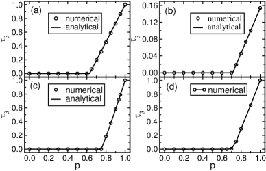
Figure 1: The three-tangle calculated with replica exchange compared to analytical results, for (a) the mixed GHZ and W states, (b) the mixed generalized GHZ and generalized W states, (c) the mixed GHZ state, W state and flipped W states with n=2, (d) the mixed GHZ state and white noise states.

The calculated $\tau_{3}$ of the mixed states are shown in Fig.1(b) for $a$=0.2, $c$=0.2, $d$=0.2. As we see the results are in excellent agreement with the analytical results. Again we find that $N_{p}$=4 is enough to the optimal results.

In the above tests, we demonstrate that our method is very effective to deal with the three-tangle of rank-2 mixed states. Recently, Jung at al. has obtained the analytical results of the three-tangle of the mixed states of GHZ, W, and flipped-W statesJung et al. (2009a). These states are of rank 3. The flipped-W states is defined as

$$|\tilde{w}\rangle=\frac{1}{\sqrt{3}}(|110\rangle+|101\rangle+|011\rangle)\,.$$ (22)

The density matrix of mixture of GHZ, W, and flipped-W states are given by,

$$\rho(p,q)=p\,|GHZ\rangle\langle GHZ|+q\,|W\rangle\langle W|+(1-p-q)\,|\tilde{W}\rangle\langle\tilde{W}|\,,$$ (23)

where $q$ was defined as $q=1-p/n$, n is a positive number. We then compared our numerical results to the analytical values. The results for the case of n=2 are shown in Fig.1(c). The numerical results are also in good agreement with the analytical results. We further calculate three-tangle of the mixed states which are of rank 4, given in Ref.Jung et al., 2009b, obtaining the same accuracy compared to the analytical results.

Table 1: Numerically calculated $\tau_{3}$ of mixed GHZ, W and flipped-W states for n=2 compared to the analytical results given in Ref. Jung et al., 2009a.

p	0.2	0.75	0.8	0.85	0.9	0.933	0.95
analytical	0	0	0.1835	0.3775	0.5805	0.7182	0.7897
numerical	5.7e-6	2e-5	0.1836	0.3781	0.5811	0.7186	0.7901

To give an illustration of the accuracy, the numerical values of mixture of GHZ, W and flipped-W state with n=2 are also listed in Table 1. We can see that all the results are within an accuracy of $\sim 10^{-4}$. The accuracy can easily be improved by increasing $\kappa$ and decreasing $T_{\rm min}$. For the example given above, in the case of p=0.8, if we reduce $T_{\rm min}$ to $10^{-10}$ and use $\kappa=10^{10}$, we obtain $\tau_{3}$=0.18349906 compared to the analytical value 0.18349861 in an accuracy $\sim 10^{-7}$. In principle, our numerical method can achieve arbitrary accuracy. We have also tried to optimize Eq. 13 via traditional CSA method. We find the performance of the traditional method is very bad, because it can easily be trapped at some local minima.

Having demonstrated the ability of the method, we then calculate the $\tau_{3}$ of the GHZ states mixed with white noise, which does not have analytical solutions so far. The density matrices of the states are

$$\rho(p)=p\,\pi_{GHZ}+\frac{1-p}{8}\,\pi_{E}\,,$$ (24)

where $\pi_{E}$ is a unit matrix. In this case, the density matrices are of rank 8. We need at least $N_{p}$=8 to ensure $R^{2}\sim$ 0. In practice, we have calculated $\tau_{3}$ up to $N_{p}$=20. We find that use $N_{p}$=15 can converge $\tau_{3}$ to less than 10^-3 for this problem. (See Fig. 2). The calculated results are shown in Fig.1(d). From Fig. 1(d), we see that $\tau_{3}$ of the white noise mixed GHZ states is zero for $p$ less than about 0.7, then increase almost linearly to 1.0 as $p$ increases. The behavior of $\tau_{3}$ looks similar to that of mixed GHZ and W states.

It is straight forward to apply the method to any mixed states. It therefore opens up a way to study the multiparticle entanglement effects in many important systems, e.g., in systems with quantum phase transitions, which was impossible before, because the analytical solution to the tree-tangle of a general mixed state is not available.

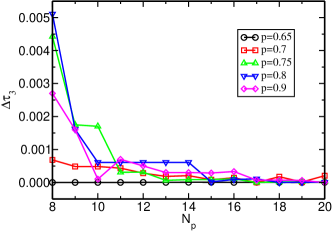
Figure 2: (Color online) The $N_{p}$ dependent $\Delta\tau_{3}$ calculated with replica exchange for density matrix constructed by GHZ state with white noise, where $\Delta\tau_{3}=\tau_{3}-\tau_{3}^{min}$ with $\tau_{3}^{min}$ the minimum three-tangle for each $p$ value.

To conclude, we have demonstrate an efficient numerical method to calculate the three-tangle of general mixed states. We construct a “energy function” (target function) for the three-tangle of the mixed state under certain constrains. The “energy function” (target function) is then optimized via a replica exchange Monte Carlo method. We have tested the method for the examples with known analytical results, showing remarkable agreement. We further calculate the three-tangle of GHZ states mixed with white noise. The work opens a way to study three-tangle of general mixed states, and can be generalized to solve many other optimization problems in quantum information theory.

L.H. acknowledges the support from the Chinese National Fundamental Research Program 2006CB921900, the Innovation funds and “Hundreds of Talents” program from Chinese Academy of Sciences, and National Natural Science Foundation of China, Grant No. 10674124. W.Z were supported by National Natural Science Foundation of China, Grant No. 10874170 and K.C.Wong Education Foundation, Hong Kong.

References

- Bennett et al. (1996) C. H. Bennett, D. DiVincenzo, J. Smolin, and W. K. Wootters, Phys. Rev. A 54, 3824 (1996).
- Coffman et al. (2000) V. Coffman, J. Kundu, and W. Wootters, Phys. Rev. A 61, 052306 (2000).
- Bai et al. (2007) Y.-K. Bai, D. Yang, and Z.-D. Wang, Phys. Rev. A 76, 022336 (2007).
- Cai et al. (2006) J.-M. Cai, Z.-W. Zhou, X.-X. Zhou, and G.-C. Guo, Phys. Rev. A 74, 042338 (2006).
- Uhlmann (2000) A. Uhlmann, Phys. Rev. A 62, 032307 (2000).
- Wooters (1998) W. K. Wooters, Phys. Rev. Lett. 80, 2245 (1998).
- Amico et al. (2008) L. Amico, R. Fazio, A. Osterloh, and V. Vedral, Rev. Mod. Phys. 80, 518 (2008).
- Lohmayer et al. (2006) R. Lohmayer, A. Osterloh, J. Siewert, and A. Uhlmann, Phys. Rev. Lett. 97, 260502 (2006).
- Eltschka et al. (2007) C. Eltschka, A. Osterloh, J. Siewert, and A. Uhlmann, arXiv:0711.4477v1 (2007).
- Jung et al. (2009a) E. Jung, M.-R. Hwang, D. Park, and J.-W. Son, Phys. Rev. A 79, 024306 (2009a).
- Jung et al. (2009b) E. Jung, D. Park, and J.-W. Son, Phys. Rev. A 80, 010301(R) (2009b).
- Swendsen and Wang (1986) R. H. Swendsen and J. S. Wang, Phys. Rev. Lett. 57, 2607 (1986).
- Geyer (1991) C. J. Geyer, Computer Science and Statistics, Proceedings of the 23rd Symposium on the interface (Interface Foundation, 1991).
- Marinari et al. (1998) E. Marinari, G. Parisi, and J. J. Ruiz-Lorenzo, Phys. Rev. B 58, 14852 (1998).
- Sugita et al. (2000) Y. Sugita, A. Kitao, and Y. Okamato, J. Chem. Phys. 113, 6042 (2000).
- Neirotti et al. (2000) J. P. Neirotti, F. Calvo, D. L. Freeman, and J. D. Doll, J. Chem. Phys. 112, 10340 (2000).
- Benatti et al. (1996) F. Benatti, H. Narnhofer, and A. Uhlmann, Rep. Math. Phys. 38, 123 (1996).
- Marinari et al. (1997) E. Marinari, G. Parisi, and J. J. Ruiz-Lorenzo, in Spin Glasses and Random Fields, edited by A. P. Young (World Scientific, Singapore, 1997).
- Kone and Kofke (2005) A. Kone and D. A. Kofke, J. Chem. Phys. 122, 206101 (2005).
- Berg (2004) B. A. Berg, Markov Chain Monte Carlo Simualtions and Their Statistical Analysis (World Scientific Press, 2004).