MedLDA: A General Framework of Maximum Margin Supervised Topic Models

Abstract

Supervised topic models utilize document’s side information for discovering predictive low dimensional representations of documents. Existing models apply the likelihood-based estimation. In this paper, we present a general framework of max-margin supervised topic models for both continuous and categorical response variables. Our approach, the maximum entropy discrimination latent Dirichlet allocation (MedLDA), utilizes the max-margin principle to train supervised topic models and estimate predictive topic representations that are arguably more suitable for prediction tasks. The general principle of MedLDA can be applied to perform joint max-margin learning and maximum likelihood estimation for arbitrary topic models, directed or undirected, and supervised or unsupervised, when the supervised side information is available. We develop efficient variational methods for posterior inference and parameter estimation, and demonstrate qualitatively and quantitatively the advantages of MedLDA over likelihood-based topic models on movie review and 20 Newsgroups data sets.

Keywords: Topic models, Maximum entropy discrimination latent Dirichlet allocation, Max-margin learning.

1 Introduction

Latent topic models such as Latent Dirichlet Allocation (LDA) (Blei et al., 2003) have recently gained much popularity in managing a large collection of documents by discovering a low dimensional representation that captures the latent semantic of the collection. LDA posits that each document is an admixture of latent topics where the topics are represented as unigram distribution over a given vocabulary. The document-specific admixture proportion is distributed as a latent Dirichlet random variable and represents a low dimensional representation of the document. This low dimensional representation can be used for tasks like classification and clustering or merely as a tool to structurally browse the otherwise unstructured collection.

The traditional LDA (Blei et al., 2003) is an unsupervised model, and thus is incapable of incorporating the useful side information associated with corpora, which is uncommon. For example, online users usually post their reviews for products or restaurants with a rating score or pros/cons rating; webpages can have their category labels; and the images in the LabelMe (Russell et al., 2008) dataset are organized in different categories and each image is associated with a set of annotation tags. Incorporating such supervised side information may guide the topic models towards discovering secondary or non-dominant statistical patterns (Chechik and Tishby, 2002), which may be more interesting or relevant to the users’ goals (e.g., predicting on unlabeled data). In contrast, the unsupervised LDA ignores such supervised information and may yields more prominent and perhaps orthogonal (to the users’ goals) latent semantic structures. This problem is serious when dealing with complex data, which usually have multiple, alternative, and conflicting underlying structures. Therefore, in order to better extract the relevant or interesting underlying structures of corpora, the supervised side information should be incorporated.

Recently, learning latent topic models with side information has gained increasing attention. Major instances include the supervised topic models (sLDA) (Blei and McAuliffe, 2007) for regression, multi-class LDA (an sLDA classification model) (Wang et al., 2009), and the discriminative LDA (DiscLDA) (Lacoste-Jullien et al., 2008) classification model. All these models focus on the document-level supervised information, such as document categories or review rating scores. Other variants of supervised topic models have been designed to deal with different application problems, such as the aspect rating model (Titov and McDonald, 2008) and the credit attribution model (Ramage et al., 2009), of which the former predicts ratings for each aspect and the latter associate each word with a label. In this paper, without loss of generality, we focus on incorporating document-level supervision information. Our learning principle can be generalized to arbitrary topic models. For the document level models, although sLDA and DiscLDA share the same goal (uncovering the latent structure in a document collection while retaining predictive power for supervised tasks), they differ in their training procedures. sLDA is trained by maximizing the joint likelihood of data and response variables while DiscLDA is trained to maximize the conditional likelihood of response variables. Furthermore, to the best of our knowledge, almost all existing supervised topic models are trained by maximizing the data likelihood.

In this paper, we propose a general principle for learning max-margin discriminative supervised latent topic models for both regression and classification. In contrast to the two-stage procedure of using topic models for prediction tasks (i.e., first discovering latent topics and then feeding them to downstream prediction models), the proposed maximum entropy discrimination latent Dirichlet allocation (MedLDA) is an integration of max-margin prediction models (e.g., support vector machines for classification) and hierarchical Bayesian topic models by optimizing a single objective function with a set of expected margin constraints. MedLDA is a special instance of PoMEN (i.e., partially observed maximum entropy discrimination Markov network) (Zhu et al., 2008b), which was proposed to combine max-margin learning and structured hidden variables in undirected Markov networks, for discovering latent topic presentations of documents. In MedLDA, the parameters for the regression or classification model are learned in a max-margin sense; and the discovery of latent topics is coupled with the max-margin estimation of the model parameters. This interplay yields latent topic representations that are more discriminative and more suitable for supervised prediction tasks.

The principle of MedLDA to do joint max-margin learning and maximum likelihood estimation is extremely general and can be applied to arbitrary topic models, including directed topic models (e.g., LDA and sLDA) or undirected Markov networks (e.g., the Harmonium (Welling et al., 2004)), unsupervised (e.g., LDA and Harmonium) or supervised (e.g., sLDA and hierarchical Harmonium (Yang et al., 2007)), and other variants of topic models with different priors, such as correlated topic models (CTMs) Blei and Lafferty (2005). In this paper, we present several examples of applying the max-margin principle to learn MedLDA models which use the unsupervised and supervised LDA as the underlying topic models to discover latent topic representations of documents for both regression and classification. We develop efficient and easy-to-implement variational methods for MedLDA, and in fact its running time is comparable to that of an unsupervised LDA for classification. This property stems from the fact that the MedLDA classification model directly optimizes the margin and does not suffer from a normalization factor which generally makes learning hard as in fully generative models such as sLDA.

The paper is structured as follows. Section 2 introduces the basic concepts of latent topic models. Section 3 and Section 4 present the MedLDA models for regression and classification respectively, with efficient variational EM algorithms. Section 5 discusses the generalization of MedLDA to other latent variable topic models. Section 6 presents empirical comparison between MedLDA and likelihood-based topic models for both regression and classification. Section 7 presents some related works. Finally, Section 8 concludes this paper with future research directions.

2 Unsupervised and Supervised Topic Models

In this section, we review the basic concepts of unsupervised and supervised topic models and two variational upper bounds which will be used later.

The unsupervised LDA (latent Dirichlet allocation) (Blei et al., 2003) is a hierarchical Bayesian model, where topic proportions for a document are drawn from a Dirichlet distribution and words in the document are repeatedly sampled from a topic which itself is drawn from those topic proportions. Supervised topic models (sLDA) (Blei and McAuliffe, 2007) introduce a response variable to LDA for each document, as illustrated in Figure 1.

Let $K$ be the number of topics and $M$ be the number of terms in a vocabulary. $\beta$ denotes a $K\times M$ matrix and each $\beta_{k}$ is a distribution over the $M$ terms. For the regression problem, where the response variable $y\in\mathbb{R}$, the generative process of sLDA is as follows:

1. Draw topic proportions $\theta|\alpha\sim\textrm{Dir}(\alpha)$.

2. For each word

   1. Draw a topic assignment $z_{n}|\theta\sim\textrm{Mult}(\theta)$.

   2. Draw a word $w_{n}|z_{n},\beta\sim\textrm{Multi}(\beta_{z_{n}})$.

3. Draw a response variable: $y|z_{1:N},\eta,\delta^{2}\sim N(\eta^{\top}\bar{z},\delta^{2})$, where $\bar{z}=1/N\sum_{n=1}^{N}z_{n}$ is the average topic proportion of a document.

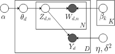
Figure 1: Supervised topic model (Blei and McAuliffe, 2007).

The model defines a joint distribution:

$$p(\theta,\mathbf{z},\mathbf{y},\mathbf{W}|\alpha,\beta,\eta,\delta^{2})=\prod_{d=1}^{D}p(\theta_{d}|\alpha)(\prod_{n=1}^{N}p(z_{dn}|\theta_{d})p(w_{dn}|z_{dn},\beta))p(y_{d}|\eta^{\top}\bar{z}_{d},\delta^{2}),$$

where $\mathbf{y}$ is the vector of response variables in a corpus $\mathcal{D}$ and $\mathbf{W}$ are all the words. The joint likelihood on $\mathcal{D}$ is $p(\mathbf{y},\mathbf{W}|\alpha,\beta,\eta,\delta^{2})$. To estimate the unknown parameters $(\alpha,\beta,\eta,\delta^{2})$, sLDA maximizes the log-likelihood $\log p(\mathbf{y},\mathbf{W}|\alpha,\beta,\eta,\delta^{2})$. Given a new document, the expected response value is the prediction:

$$\hat{y}\triangleq E[Y|w_{1:N},\alpha,\beta,\eta,\delta^{2}]=\eta^{\top}E[\bar{Z}|w_{1:N},\alpha,\beta,\delta^{2}],$$ (1)

where $E[X]$ is an expectation with respect to the posterior distribution of the random variable $X$.

Since exact inference of the posterior distribution of hidden variables and the likelihood is intractable, variational methods (Jordan et al., 1999) are applied to get approximate solutions. Let $q(\theta,\mathbf{z}|\gamma,\phi)$ be a variational distribution that approximates the posterior $p(\theta,\mathbf{z}|\alpha,\beta,\eta,\delta^{2},\mathbf{y},\mathbf{W})$. By using Jensen’s inequality, we can get a variational upper bound of the negative log-likelihood:

$$\mathcal{L}^{s}(q)=-E_{q}[\log p(\theta,\mathbf{z},\mathbf{y},\mathbf{W}|\alpha,\beta,\eta,\delta^{2})]-\mathcal{H}(q(\mathbf{z},\theta))\geq-\log p(\mathbf{y},\mathbf{W}|\alpha,\beta,\eta,\delta^{2}),$$

where $\mathcal{H}(q)\triangleq-E_{q}[\log q]$ is the entropy of $q$. By introducing some independence assumptions (like mean field) about the $q$ distribution, this upper bound can be efficiently optimized, and we can estimate the parameters $(\alpha,\beta,\eta,\delta^{2})$ and get the best approximation $q$. See (Blei and McAuliffe, 2007) for more details.

For the unsupervised LDA, the generative procedure is similar, but without the third step. The joint distribution is $p(\theta,\mathbf{z},\mathbf{W}|\alpha,\beta)=\prod_{d=1}^{D}p(\theta_{d}|\alpha)(\prod_{n=1}^{N}p(z_{dn}|\theta_{d})p(w_{dn}|z_{dn},\beta))$ and the likelihood is $p(\mathbf{W}|\alpha,\beta)$. Similarly, a variational upper bound can be derived for approximate inference:

$$\mathcal{L}^{u}(q)=-E_{q}[\log p(\theta,\mathbf{z},\mathbf{W}|\alpha,\beta)]-\mathcal{H}(q(\mathbf{z},\theta))\geq-\log p(\mathbf{W}|\alpha,\beta),$$

where $q(\theta,\mathbf{z})$ is a variational distribution that approximates the posterior $p(\theta,\mathbf{z}|\alpha,\beta,\mathbf{W})$. Again, by making some independence assumptions, parameter estimation and posterior inference can be efficiently done by optimizing $\mathcal{L}^{u}(q)$. See (Blei et al., 2003) for more details.

In sLDA, by changing the distribution model of generating response variables, other types of responses can be modeled, such as the discrete classification problem (Blei and McAuliffe, 2007; Wang et al., 2009). However, the posterior inference and parameter estimation in supervised LDA classification model are much more difficult than those of the sLDA regression model because of the normalization factor of the non-Gaussian distribution model for response variables. Variational methods or multi-delta methods were used to approximate the normalization factor (Wang et al., 2009; Blei and McAuliffe, 2007). DiscLDA (Lacoste-Jullien et al., 2008) is a discriminative variant of supervised topic models for classification, where the unknown parameters (i.e., a linear transformation matrix) are learned by maximizing the conditional likelihood of the response variables.

Although both maximum likelihood estimation (MLE) and maximum conditional likelihood estimation (MCLE) have shown great success in many cases, the max-margin learning is arguably more discriminative and closer to our final prediction task in supervised topic models. Empirically, max-margin methods like the support vector machines (SVMs) for classification have demonstrated impressive success in a wide range of tasks, including image classification, character recognition, etc. In addition to the empirical success, max-margin methods enjoy strong generalization guarantees, and are able to use kernels, allowing the classifier to deal with a very high-dimensional feature space.

To integrate the advantages of max-margin methods into the procedure of discovering latent topics, below, we present a max-margin variant of the supervised topic models, which can discover predictive topic representations that are more suitable for supervised prediction tasks, e.g., regression and classification.

3 Maximum Entropy Discrimination LDA for Regression

In this section, we consider the supervised prediction task, where the response variables take continuous real values. This is known as a regression problem in machine learning. We present two MedLDA regression models that perform max-margin learning for the supervised LDA and unsupervised LDA models. Before diving into the full exposition of our methods, we first review the basic support vector regression method, upon which MedLDA is built.

3.1 Support Vector Regression

Support vector machines have been developed for both classification and regression. In this section, we consider the support vector regression (SVR), on which a comprehensive tutorial has been published by Smola and Sch$\ddot{o}$lkopf (2003). Here, we provide a brief recap of the basic concepts.

Suppose we are given a training set $\mathcal{D}=\{(\mathbf{x}_{1},y_{1}),\cdots,(\mathbf{x}_{D},y_{D})\}$, where $\mathbf{x}\in\mathcal{X}$ are inputs and $y\in\mathbb{R}$ are real response values. In $\epsilon$-support vector regression (Vapnik, 1995), our goal is to find a function $h(\mathbf{x})\in\mathcal{F}$ that has at most $\epsilon$ deviation from the true response values $y$ for all the training data, and at the same time as flat as possible. One common choice of the function family $\mathcal{F}$ is the linear functions, that is, $h(\mathbf{x})=\eta^{\top}\mathbf{f}(\mathbf{x})$, where $\mathbf{f}=\{f_{1},\cdots,f_{K}\}$ is a vector of feature functions. Each $f_{k}:\mathcal{X}\to\mathbb{R}$ is a feature function. $\eta$ is the corresponding weight vector. Formally, the linear SVR finds an optimal linear function by solving the following constrained convex optimization problem

$${\rm P0(SVR)}: \min_{\eta,\xi,\xi^{\star}}~{}\frac{1}{2}\|\eta\|_{2}^{2}+C\sum_{d=1}^{D}(\xi_{d}+\xi_{d}^{\star})$$

$$\mathrm{s.t.}~{}\forall d: \left\{\begin{array}[]{rl}y_{d}-\eta^{\top}\mathbf{f}(\mathbf{x}_{d})&\leq\epsilon+\xi_{d}\\ -y_{d}+\eta^{\top}\mathbf{f}(\mathbf{x}_{d})&\leq\epsilon+\xi_{d}^{\star}\\ \xi_{d},\xi_{d}^{\star}&\geq 0\end{array}\right.,$$ (5)

where $\|\eta\|_{2}^{2}=\eta^{\top}\eta$ is the $\ell_{2}$-norm; $\xi$ and $\xi^{\star}$ are slack variables that tolerates some errors in the training data; and $\epsilon$ is the precision parameter. The positive regularization constant $C$ determines the trade-off between the flatness of $h$ (represented by the $\ell_{2}$-norm) and the amount up to which deviations larger than $\epsilon$ are tolerated. The problem P0 can be equivalently formulated as a regularized empirical loss minimization, where the loss is the so-called $\epsilon$-insensitive loss (Smola and Sch$\ddot{o}$lkopf, 2003).

For the standard SVR optimization problem, P0 is a QP problem and can be easily solved in the dual formulation. In the Lagrangian method, samples with non-zero lagrange multipliers are called support vectors, the same as in SVM classification model. There are also some freely available packages for solving a standard SVR problem, such as the SVM-light (Joachims, 1999). We will use these methods as a sub-routine to solve our proposed approach.

3.2 Learning MedLDA for Regression

Instead of learning a point estimate of $\eta$ as in sLDA, we take a more general Bayesian-style (i.e., an averaging model) approach and learn a distribution $q(\eta)$ in a max-margin manner. For prediction, we take the average over all the possible models (represented by $\eta$):

$$\hat{y}\triangleq E[Y|w_{1:N},\alpha,\beta,\delta^{2}]=E[\eta^{\top}\bar{Z}|w_{1:N},\alpha,\beta,\delta^{2}].$$ (6)

Now, the question underlying the averaging prediction rule (6) is how we can devise an appropriate loss function and constraints to integrate the max-margin concepts of SVR into latent topic discovery. In the sequel, we present the maximum entropy discrimination latent Dirichlet allocation (MedLDA), which is an extension of the PoMEN (i.e., partially observed maximum entropy discrimination Markov networks) (Zhu et al., 2008b) framework. PoMEN is an elegant combination of max-margin learning with structured hidden variables in Markov networks. The MedLDA is an extension of PoMEN to learn directed Bayesian networks with latent variables, in particular the latent topic models, which discover latent semantic structures of document collections.

There are two principled choice points in MedLDA according to the prediction rule (6): (1) the distribution of model parameter $\eta$; and (2) the distribution of latent topic assignment $Z$. Below, we present two MedLDA regression models by using supervised LDA or unsupervised LDA to discover the latent topic assignment $Z$. Accordingly, we denote these two models as MedLDA${}^{r}_{full}$ and MedLDA${}^{r}_{partial}$.

3.2.1 Max-Margin Training of sLDA

For regression, the MedLDA is defined as an integration of a Bayesian sLDA, where the parameter $\eta$ is sampled from a prior $p_{0}(\eta)$, and the $\epsilon$-insensitive support vector regression (SVR) (Smola and Sch$\ddot{o}$lkopf, 2003). Thus, MedLDA defines a joint distribution: $p(\theta,\mathbf{z},\eta,\mathbf{y},\mathbf{W}|\alpha,\beta,\delta^{2})=p_{0}(\eta)p(\theta,\mathbf{z},\mathbf{y},\mathbf{W}|\alpha,\beta,\eta,\delta^{2})$, where the second term is the same as in the sLDA. Since directly optimizing the log likelihood is intractable, as in sLDA, we optimize its upper bound. Different from sLDA, $\eta$ is a random variable now. So, we define the variational distribution $q(\theta,\mathbf{z},\eta|\gamma,\phi)$ to approximate the true posterior $p(\theta,\mathbf{z},\eta|\alpha,\beta,\delta^{2},\mathbf{y},\mathbf{W})$. Then, the upper bound of the negative log-likelihood $-\log p(\mathbf{y},\mathbf{W}|\alpha,\beta,\delta^{2})$ is

$$\mathcal{L}^{bs}(q)\triangleq-E_{q}[\log p(\theta,\mathbf{z},\eta,\mathbf{y},\mathbf{W}|\alpha,\beta,\delta^{2})]-\mathcal{H}(q(\theta,\mathbf{z},\eta))=KL(q(\eta)\|p_{0}(\eta))+E_{q(\eta)}[\mathcal{L}^{s}],$$ (7)

where $KL(p\|q)=E_{p}[\log(p/q)]$ is the Kullback-Leibler (KL) divergence.

Thus, the integrated learning problem is defined as:

$${\rm P1(MedLDA}^{r}_{full}): \min_{q,\alpha,\beta,\delta^{2},\xi,\xi^{\star}}~{}\mathcal{L}^{bs}(q)+C\sum_{d=1}^{D}(\xi_{d}+\xi_{d}^{\star})$$

$$\mathrm{s.t.}~{}\forall d: \left\{\begin{array}[]{rll}y_{d}-E[\eta^{\top}\bar{Z}_{d}]&\leq\epsilon+\xi_{d},&\mu_{d}\\ -y_{d}+E[\eta^{\top}\bar{Z}_{d}]&\leq\epsilon+\xi_{d}^{\star},&\mu_{d}^{\star}\\ \xi_{d}&\geq 0,&v_{d}\\ \xi_{d}^{\star}&\geq 0,&v_{d}^{\star}\end{array}\right.$$ (12)

where $\mu,\mu^{\star},v,v^{\star}$ are lagrange multipliers; $\xi,\xi^{\star}$ are slack variables absorbing errors in training data; and $\epsilon$ is the precision parameter. The constraints in P1 are in the same form as those of P0, but in an expected version because both the latent topic assignments $Z$ and the model parameters $\eta$ are random variables in MedLDA. Similar as in SVR, the expected constraints correspond to an $\epsilon$-insensitive loss, that is, if the current prediction $\hat{y}$ as in Eq. (6) does not deviate from the target value too much (i.e., less than $\epsilon$), there is no loss; otherwise, a linear loss will be penalized.

The rationale underlying the MedLDA${}^{r}_{full}$ is that: let the current model be $p(\theta,\mathbf{z},\eta,\mathbf{y},\mathbf{W}|\alpha,\beta,\delta^{2})$, then we want to find a latent topic representation and a model distribution (as represented by the distribution $q$) which on one hand tend to predict correctly on the data with a sufficient large margin, and on the other hand tend to explain the data well (i.e., minimizing an variational upper bound of the negative log-likelihood). The max-margin estimation and topic discovery procedure are coupled together via the constraints, which are defined on the expectations of model parameters $\eta$ and the latent topic representations $Z$. This interplay will yield a topic representation that is more suitable for max-margin learning, as explained below.

Variational EM-Algorithm: Solving the constrained problem P1 is generally intractable. Thus, we make use of mean-field variational methods (Jordan et al., 1999) to efficiently obtain an approximate $q$. The basic principle of mean-field variational methods is to form a factorized distribution of the latent variables, parameterized by free variables which are called variational parameters. These parameters are fit so that the KL divergence between the approximate $q$ and the true posterior is small. Variational methods have successfully used in many topic models, as we have presented in Section 2.

As in standard topic models, we assume $q(\theta,\mathbf{z},\eta|\gamma,\phi)=q(\eta)\prod_{d=1}^{D}q(\theta_{d}|\gamma_{d})\prod_{n=1}^{N}q(z_{dn}|\phi_{dn})$, where $\gamma_{d}$ is a $K$-dimensional vector of Dirichlet parameters and each $\phi_{dn}$ is a categorical distribution over $K$ topics. Then, $E[Z_{dn}]=\phi_{dn}$, $E[\eta^{\top}\bar{Z}_{d}]=E[\eta]^{\top}(1/N)\sum_{n=1}^{N}\phi_{dn}$. We can develop an EM algorithm, which iteratively solves the following two steps: E-step: infer the posterior distribution of the hidden variables $\theta$, $Z$, and $\eta$; and M-step: estimate the unknown model parameters $\alpha$, $\beta$, and $\delta^{2}$.

The essential difference between MedLDA and sLDA lies in the E-step to infer the posterior distribution of $\mathbf{z}$ and $\eta$ because of the margin constraints in P1. As we shall see in Eq. (14), these constraints will bias the expected topic proportions towards the ones that are more suitable for the supervised prediction tasks. Since the constraints in P1 are not on the model parameters ($\alpha$, $\beta$, and $\delta^{2}$), the M-step is similar to that of the sLDA. We outline the algorithm in Alg. 1 and explain it in details below. Specifically, we formulate a Lagrangian $L$ for P1

$$L= \mathcal{L}^{bs}(q)+C\sum_{d=1}^{D}(\xi_{d}+\xi_{d}^{\star})-\sum_{d=1}^{D}\mu_{d}(\epsilon+\xi_{d}-y_{d}+E[\eta^{\top}\bar{Z}_{d}])-\sum_{d=1}^{D}(\mu_{d}^{\star}(\epsilon+\xi_{d}^{\star}+y_{d}-E[\eta^{\top}\bar{Z}_{d}])$$

$$+v_{d}\xi_{d}+v_{d}^{\star}\xi_{d}^{\star})-\sum_{d=1}^{D}\sum_{i=1}^{N}c_{di}(\sum_{j=1}^{K}\phi_{dij}-1),$$

where the last term is due to the normalization condition $\sum_{j=1}^{K}\phi_{dij}=1,~{}\forall i,d$. Then, the EM procedure alternatively optimize the Lagrangian functional with respect to each argument.

1. E-step: we infer the posterior distribution of the latent variables $\theta$, $Z$ and $\eta$. For the variables $\theta$ and $Z$, inferring the posterior distribution is to fit the variational parameters $\gamma$ and $\phi$ because of the mean-field assumption about $q$, but for $\eta$ the optimization is on $q(\eta)$. Specifically, we have the following update rules for different latent variables.

   Algorithm 1 Variational MedLDA^r

     Input: corpus $\mathcal{D}=\{(\mathbf{y},\mathbf{W})\}$, constants $C$ and $\epsilon$, and topic number $K$.

     Output: Dirichlet parameters $\gamma$, posterior distribution $q(\eta)$, parameters $\alpha$, $\beta$ and $\delta^{2}$.

     repeat

        /**** E-Step ****/

        for $d=1$ to $D$ do

           Update $\gamma_{d}$ as in Eq. (13).

           for $i=1$ to $N$ do

              Update $\phi_{di}$ as in Eq. (14).

           end for

        end for

        Solve the dual problem D1 to get $q(\eta)$, $\mu$ and $\mu^{\star}$.

        /**** M-Step ****/

        Update $\beta$ using Eq. (24), and update $\delta^{2}$ using Eq. (25). $\alpha$ is fixed as $1/K$ times the ones vector.

     until convergence

   Since the constraints in P1 are not on $\gamma$, optimize $L$ with respect to $\gamma_{d}$ and we can get the same update formula as in sLDA:

   $$\gamma_{d}\leftarrow\alpha+\sum_{n=1}^{N}\phi_{dn}$$ (13)

   Due to the fully factorized assumption of $q$, for each document $d$ and each word $i$, by setting $\partial L/\partial\phi_{di}=0$, we have:

   $$\phi_{di}\propto\exp\big{(}E[\log\theta|\gamma]+E[\log p(w_{di}|\beta)] +\frac{y_{d}}{N\delta^{2}}E[\eta]-\frac{2E[\eta^{\top}\phi_{d,-i}\eta]+E[\eta\circ\eta]}{2N^{2}\delta^{2}}$$ (14)

   $$+\frac{E[\eta]}{N}(\mu_{d}-\mu_{d}^{\star})\big{)},$$

   where $\phi_{d,-i}=\sum_{n\neq i}\phi_{dn}$; $\eta\circ\eta$ is the element-wise product; and the result of exponentiating a vector is a vector of the exponentials of its corresponding components. The first two terms in the exponential are the same as those in unsupervised LDA.

   The essential differences of MedLDA^r from the sLDA lie in the last three terms in the exponential of $\phi_{di}$. Firstly, the third and fourth terms are similar to those of sLDA, but in an expected version since we are learning the distribution $q(\eta)$. The second-order expectations $E[\eta^{\top}\phi_{d,-i}\eta]$ and $E[\eta\circ\eta]$ mean that the co-variances of $\eta$ affect the distribution over topics. This makes our approach significantly different from a point estimation method, like sLDA, where no expectations or co-variances are involved in updating $\phi_{di}$. Secondly, the last term is from the max-margin regression formulation. For a document $d$, which lies around the decision boundary, i.e., a support vector, either $\mu_{d}$ or $\mu_{d}^{\star}$ is non-zero, and the last term biases $\phi_{di}$ towards a distribution that favors a more accurate prediction on the document. Moreover, the last term is fixed for words in the document and thus will directly affect the latent representation of the document, i.e., $\gamma_{d}$. Therefore, the latent representation by MedLDA^r is more suitable for max-margin learning.

   Let $A$ be the $D\times K$ matrix whose rows are the vectors $\bar{Z}_{d}^{\top}$. Then, we have the following theorem.

   Theorem 1

   For MedLDA, the optimum solution of $q(\eta)$ has the form:

   $$q(\eta)=\frac{p_{0}(\eta)}{Z}\exp\big{(}\eta^{\top}\sum_{d=1}^{D}(\mu_{d}-\mu_{d}^{\star}+\frac{y_{d}}{\delta^{2}})E[\bar{Z}_{d}]-\eta^{\top}\frac{E[A^{\top}A]}{2\delta^{2}}\eta\big{)}$$

   where $E[A^{\top}A]=\sum_{d=1}^{D}E[\bar{Z}_{d}\bar{Z}_{d}^{\top}]$, and $E[\bar{Z}_{d}\bar{Z}_{d}^{\top}]=\frac{1}{N^{2}}(\sum_{n=1}^{N}\sum_{m\neq n}\phi_{dn}\phi_{dm}^{\top}+\sum_{n=1}^{N}{\rm diag}\{\phi_{dn}\})$. The lagrange multipliers are the solution of the dual problem of P1:

   $${\rm D1}: \max_{\mu,\mu^{\star}}~{}-\log Z-\epsilon\sum_{d=1}^{D}(\mu_{d}+\mu_{d}^{\star})+\sum_{d=1}^{D}y_{d}(\mu_{d}-\mu_{d}^{\star})$$

   $$\mathrm{s.t.}~{}~{}\forall d:~{}\mu_{d},\mu_{d}^{\star}\in[0,C].$$

   Proof (sketch) Set the partial derivative $\partial L/\partial q(\eta)$ equal zero, we can get the solution of $q(\eta)$. Plugging $q(\eta)$ into $L$, we get the dual problem.  
   

   In MedLDA^r, we can choose different priors to introduce some regularization effects. For the standard normal prior: $p_{0}(\eta)=\mathcal{N}(0,I)$, we have the corollary:

   Corollary 2

   Assume the prior $p_{0}(\eta)=\mathcal{N}(0,I)$, then the optimum solution of $q(\eta)$ is

   $$q(\eta)=\mathcal{N}\big{(}\lambda,\Sigma\big{)},$$ (15)

   where $\lambda=\Sigma\big{(}\sum_{d=1}^{D}(\mu_{d}-\mu_{d}^{\star}+\frac{y_{d}}{\delta^{2}})E[\bar{Z}_{d}]\big{)}$ is the mean and $\Sigma=(I+1/\delta^{2}E[A^{\top}A])^{-1}$ is a $K\times K$ co-variance matrix. The dual problem of P1 is:

   $$\max_{\mu,\mu^{\star}}~{}-\frac{1}{2}a^{\top}\Sigma a-\epsilon\sum_{d=1}^{D}(\mu_{d}+\mu_{d}^{\star})+\sum_{d=1}^{D}y_{d}(\mu_{d}-\mu_{d}^{\star})$$

   $$\mathrm{s.t.}~{}~{}\forall d:~{}\mu_{d},\mu_{d}^{\star}\in[0,C],$$

   where $a=\sum_{d=1}^{D}(\mu_{d}-\mu_{d}^{\star}+\frac{y_{d}}{\delta^{2}})E[\bar{Z}_{d}]$.

   In the above Corollary, computation of $\Sigma$ can be achieved robustly through Cholesky decomposition of $\delta^{2}I+E[A^{\top}A]$, an $O(K^{3})$ procedure. Another example is the Laplace prior, which can lead to a shrinkage effect (Zhu et al., 2008a) that is useful in sparse problems. In this paper, we focus on the normal prior and extension to the Laplace prior can be done similarly as in (Zhu et al., 2008a). For the standard normal prior, the dual optimization problem is a QP problem and can be solved with any standard QP solvers, although they may not be so efficient. To leverage recent developments in support vector regression, we first prove the following corollary:

   Corollary 3

   Assume the prior $p_{0}(\eta)=\mathcal{N}(0,I)$, then the mean $\lambda$ of $q(\eta)$ is the optimum solution of the following problem:

   $$\min_{\lambda,\xi,\xi^{\star}} \frac{1}{2}\lambda^{\top}\Sigma^{-1}\lambda-\lambda^{\top}(\sum_{d=1}^{D}\frac{y_{d}}{\delta^{2}}E[\bar{Z}_{d}])+C\sum_{d=1}^{D}(\xi_{d}+\xi_{d}^{\star})$$

   $$\mathrm{s.t.}~{}\forall d: \left\{\begin{array}[]{rl}y_{d}-\lambda^{\top}E[\bar{Z}_{d}]&\leq\epsilon+\xi_{d}\\ -y_{d}+\lambda^{\top}E[\bar{Z}_{d}]&\leq\epsilon+\xi_{d}^{\star}\\ \xi_{d},\xi_{d}^{\star}&\geq 0\end{array}\right.$$ (19)

   Proof  See Appendix A for details.  
   

   The above primal form can be re-formulated as a standard SVR problem and solved by using existing algorithms like SVM-light (Joachims, 1999) to get $\lambda$ and the dual parameters $\mu$ and $\mu^{\star}$. Specifically, we do Cholesky decomposition $\Sigma^{-1}=U^{\top}U$, where $U$ is an upper triangular matrix with strict positive diagonal entries. Let $\nu=\sum_{d=1}^{D}\frac{y_{d}}{\delta^{2}}E[\bar{Z}_{d}]$, and we define $\lambda^{\prime}=U(\lambda-\Sigma\nu)$; $y_{d}^{\prime}=y_{d}-\nu^{\top}\Sigma E[\bar{Z}_{d}]$; and $\mathbf{x}_{d}=(U^{-1})^{\top}E[\bar{Z}_{d}]$. Then, the above primal problem in Corollary 3 can be re-formulated as the following standard form:

   $$\min_{\lambda^{\prime},\xi,\xi^{\star}} \frac{1}{2}\|\lambda^{\prime}\|_{2}^{2}+C\sum_{d=1}^{D}(\xi_{d}+\xi_{d}^{\star})$$

   $$\mathrm{s.t.}~{}\forall d: \left\{\begin{array}[]{rl}y_{d}^{\prime}-(\lambda^{\prime})^{\top}\mathbf{x}_{d}&\leq\epsilon+\xi_{d}\\ -y_{d}^{\prime}+(\lambda^{\prime})^{\top}\mathbf{x}_{d}&\leq\epsilon+\xi_{d}^{\star}\\ \xi_{d},\xi_{d}^{\star}&\geq 0\end{array}\right.$$ (23)

2. M-step: Now, we estimate the unknown parameters $\alpha,~{}\beta$, and $\delta^{2}$. Here, we assume $\alpha$ is fixed. For $\beta$, the update equations are the same as for sLDA:

   $$~{}~{}~{}~{}~{}\beta_{k,w}\propto\sum_{d=1}^{D}\sum_{n=1}^{N}1(w_{dn}=w)\phi_{dnk},$$ (24)

   For $\delta^{2}$, this step is similar to that of sLDA but in an expected version. The update rule is:

   $$\delta^{2}\leftarrow\frac{1}{D}\big{(}\mathbf{y}^{\top}\mathbf{y}-2\mathbf{y}^{\top}E[A]E[\eta]+E[\eta^{\top}E[A^{\top}A]\eta]\big{)},$$ (25)

   where $E[\eta^{\top}E[A^{\top}A]\eta]={\rm tr}(E[A^{\top}A]E[\eta\eta^{\top}])$.

3.2.2 Max-Margin Learning of LDA for Regression

In the previous section, we have presented the MedLDA regression model which uses the supervised sLDA to discover the latent topic representations $Z$. The same principle can be applied to perform joint maximum likelihood estimation and max-margin training for the unsupervised LDA Blei et al. (2003). In this section, we present this MedLDA model, which will be referred to as MedLDA${}^{r}_{partial}$.

A naive approach to using the unsupervised LDA for supervised prediction tasks, e.g., regression, is a two-step procedure: (1) using the unsupervised LDA to discover the latent topic representations of documents; and (2) feeding the low-dimensional topic representations into a regression model (e.g., SVR) for training and testing. This de-coupled approach is rather sub-optimal because the side information of documents (e.g., rating scores of movie reviews) is not used in discovering the low-dimensional representations and thus can result in a sub-optimal representation for prediction tasks. Below, we present the MedLDA${}^{r}_{partial}$, which integrates an unsupervised LDA for discovering topics with the SVR for regression. The inter-play between topic discovery and supervised prediction will result in more discriminative latent topic representations, similar as in MedLDA${}^{r}_{full}$.

When the underlying topic model is the unsupervised LDA, the likelihood is $p(\mathbf{W}|\alpha,\beta)$ as we have stated. For regression, we apply the $\epsilon$-insensitive support vector regression (SVR) Smola and Sch$\ddot{o}$lkopf (2003) approach as before. Again, we learn a distribution $q(\eta)$. The prediction rule is the same as in Eq. (6). The integrated learning problem is defined as:

$${\rm P2(MedLDA}^{r}_{\it partial}): \min_{q,q(\eta),\alpha,\beta,\xi,\xi^{\star}}~{}\mathcal{L}^{u}(q)+KL(q(\eta)||p_{0}(\eta))+C\sum_{d=1}^{D}(\xi_{d}+\xi_{d}^{\star})$$

$$\mathrm{s.t.}~{}\forall d: \left\{\begin{array}[]{rl}y_{d}-E[\eta^{\top}\bar{Z}_{d}]&\leq\epsilon+\xi_{d}\\ -y_{d}+E[\eta^{\top}\bar{Z}_{d}]&\leq\epsilon+\xi_{d}^{\star}\\ \xi_{d},\xi_{d}^{\star}&\geq 0\end{array}\right.,$$ (29)

where the $KL$-divergence is a regularizer that bias the estimate of $q(\eta)$ towards the prior. In MedLDA${}^{r}_{\it full}$, this KL-regularizer is implicitly contained in the variational bound $\mathcal{L}^{bs}$ as shown in Eq. (7).

Variational EM-Algorithm: For MedLDA${}^{r}_{\it partial}$, the constrained optimization problem P2 can be similarly solved with an EM procedure. Specifically, we make the same independence assumptions about $q$ as in LDA (Blei et al., 2003), that is, we assume that $q(\theta,\mathbf{z}|\gamma,\phi)=\prod_{d=1}^{D}q(\theta_{d}|\gamma_{d})\prod_{n=1}^{N}q(z_{dn}|\phi_{dn})$, where the variational parameters $\gamma$ and $\phi$ are the same as in MedLDA${}^{r}_{\it full}$. By formulating a Lagrangian $L$ for P2 and iteratively optimizing $L$ over each variable, we can get a variational EM-algorithm that is similar to that of MedLDA${}^{r}_{full}$.

1. E-step: The update rule for $\gamma$ is the same as in MedLDA${}^{r}_{\it full}$. For $\phi$, by setting $\partial L/\partial\phi_{di}=0$, we have:

   $$\phi_{di}\propto\exp\big{(}E[\log\theta|\gamma]+E[\log p(w_{di}|\beta)]+\frac{E[\eta]}{N}(\mu_{d}-\mu_{d}^{\star})\big{)},$$ (30)

   Compared to the Eq. (14), Eq. (30) is simpler and does not have the complex third and fourth terms of Eq. (14). This simplicity suggests that the latent topic representation is less affected by the max-margin estimation (i.e., the prediction model’s parameters).

   Set $\partial L/\partial q(\eta)=0$, then we get:

   $$q(\eta)=\frac{p_{0}(\eta)}{Z}\exp\big{(}\eta^{\top}\sum_{d=1}^{D}(\mu_{d}-\mu_{d}^{\star})E[\bar{Z}_{d}]\big{)}$$

   Plugging $q(\eta)$ into $L$, the dual problem D2 is the same as D1. Again, we can choose different priors to introduce some regularization effects. For the standard normal prior: $p_{0}(\eta)=\mathcal{N}(0,I)$, the posterior is also a normal: $q(\eta)=\mathcal{N}(\lambda,I)$, where $\lambda=\sum_{d=1}^{D}(\mu_{d}-\mu_{d}^{\star})E[\bar{Z}_{d}]$ is the mean. This identity covariance matrix is much simpler than the covariance matrix $\Sigma$ as in MedLDA${}^{r}_{full}$, which depends on the latent topic representation $Z$. Since $I$ is independent of $Z$, the prediction model in MedLDA${}^{r}_{partial}$ is less affected by the latent topic representations. Together with the simpler update rule (30), we can conclude that the coupling between the max-margin estimation and the discovery of latent topic representations in MedLDA${}^{r}_{partial}$ is loser than that of the MedLDA${}^{r}_{full}$. The loser coupling will lead to inferior empirical performance as we shall see.

   For the standard normal prior, the dual problem ${\rm D2}$ is a QP problem:

   $$\max_{\mu,\mu^{\star}}~{}-\frac{1}{2}\|\lambda\|_{2}^{2}-\epsilon\sum_{d=1}^{D}(\mu_{d}+\mu_{d}^{\star})+\sum_{d=1}^{D}y_{d}(\mu_{d}-\mu_{d}^{\star})$$

   $$\mathrm{s.t.}~{}~{}\forall d:~{}\mu_{d},\mu_{d}^{\star}\in[0,C],$$

   Similarly, we can derive its primal form, which can be reformulated as a standard SVR problem:

   $$\min_{\lambda,\xi,\xi^{\star}} \frac{1}{2}\|\lambda\|_{2}^{2}-\lambda^{\top}(\sum_{d=1}^{D}\frac{y_{d}}{\delta^{2}}E[\bar{Z}_{d}])+C\sum_{d=1}^{D}(\xi_{d}+\xi_{d}^{\star})$$

   $$\mathrm{s.t.}~{}\forall d: \left\{\begin{array}[]{rl}y_{d}-\lambda^{\top}E[\bar{Z}_{d}]&\leq\epsilon+\xi_{d}\\ -y_{d}+\lambda^{\top}E[\bar{Z}_{d}]&\leq\epsilon+\xi_{d}^{\star}\\ \xi_{d},\xi_{d}^{\star}&\geq 0.\end{array}\right.$$ (34)

   Now, we can leverage recent developments in support vector regression to solve either the dual problem or the primal problem.

2. M-step: the same as in the MedLDA${}^{r}_{\it full}$.

4 Maximum Entropy Discrimination LDA for Classification

In this section, we consider the discrete response variable and present the MedLDA classification model.

4.1 Learning MedLDA for Classification

For classification, the response variables $y$ are discrete. For brevity, we only consider the multi-class classification, where $y\in\{1,\cdots,M\}$. The binary case can be easily defined based on a binary SVM and the optimization problem can be solved similarly.

For classification, we assume the discriminant function $F$ is linear, that is, $F(y,z_{1:N},\eta)=\eta_{y}^{\top}\bar{z}$, where $\bar{z}=1/N\sum_{n}z_{n}$ as in the regression model, $\eta_{y}$ is a class-specific $K$-dimensional parameter vector associated with the class $y$ and $\eta$ is a $MK$-dimensional vector by stacking the elements of $\eta_{y}$. Equivalently, $F$ can be written as $F(y,z_{1:N},\eta)=\eta^{\top}\mathbf{f}(y,\bar{z})$, where $\mathbf{f}(y,\bar{z})$ is a feature vector whose components from $(y-1)K+1$ to $yK$ are those of the vector $\bar{z}$ and all the others are 0. From each single $F$, a prediction rule can be derived as in SVM. Here, we consider the general case to learn a distribution of $q(\eta)$ and for prediction, we take the average over all the possible models and the latent topics:

$$y^{\star}={\rm arg}\max_{y}E[\eta^{\top}\mathbf{f}(y,\bar{Z})|\alpha,\beta].$$ (35)

Now, the problem is to learn an optimal set of parameters $\alpha,\beta$ and distribution $q(\eta)$. Below, we present the MedLDA classification model. In principle, we can develop two variants of MedLDA classification models, which use the supervised sLDA (Wang et al., 2009) and the unsupervised LDA to discover latent topics as in the regression case. However, for the case of using supervised sLDA for classification, it is impossible to derive a dual formulation of its optimization problem because of the normalized non-Gaussian prediction model (Blei and McAuliffe, 2007; Wang et al., 2009). Here, we consider the case where we use the unsupervised LDA as the underlying topic model to discover the latent topic representation $Z$. As we shall see, the MedLDA classification model can be easily learned by using existing SVM solvers to optimize its dual optimization problem.

4.1.1 Max-Margin Learning of LDA for Classification

As we have stated, the supervised sLDA model has a normalization factor that makes the learning generally intractable, except for some special cases like the normal distribution as in the regression case. In (Blei and McAuliffe, 2007; Wang et al., 2009), variational methods or high-order Taylor expansion is applied to approximate the normalization factor in classification model. In our max-margin formulation, since our target is to directly minimize a hinge loss, we do not need a normalized distribution model for the response variables $Y$. Instead, we define a partially generative model on $(\theta,\mathbf{z},\mathbf{W})$ only as in the unsupervised LDA, and for the classification (i.e., from $Z$ to $Y$), we apply the max-margin principle, which does not require a normalized distribution. Thus, in this case, the likelihood of the corpus $\mathcal{D}$ is $p(\mathbf{W}|\alpha,\beta)$.

Similar as in the MedLDA${}^{r}_{\it partial}$ regression model, we define the integrated latent topic discovery and multi-class classification model as follows:

$${\rm P3(MedLDA^{c})}: \min_{q,q(\eta),\alpha,\beta,\xi}\mathcal{L}^{u}(q)+KL(q(\eta)||p_{0}(\eta))+C\sum_{d=1}^{D}\xi_{d}$$

$$\mathrm{s.t.}~{}\forall d,~{}y\neq y_{d}: ~{}~{}~{}~{}E[\eta^{\top}\Delta\mathbf{f}_{d}(y)]\geq 1-\xi_{d};~{}\xi_{d}\geq 0,$$

where $q(\theta,\mathbf{z}|\gamma,\phi)$ is a variational distribution; $\mathcal{L}^{u}(q)$ is a variational upper bound of $-\log p(\mathbf{W}|\alpha,\beta)$; $\Delta\mathbf{f}_{d}(y)=\mathbf{f}(y_{d},\bar{Z}_{d})-\mathbf{f}(y,\bar{Z}_{d})$, and $\xi$ are slack variables. $E[\eta^{\top}\Delta\mathbf{f}_{d}(y)]$ is the “expected margin” by which the true label $y_{d}$ is favored over a prediction $y$. These margin constraints make MedLDA^c fundamentally different from the mixture of conditional max-entropy models (Pavlov et al., 2003), where constraints are based on moment matching, i.e., empirical expectations of features are equal to their model expectations.

The rationale underlying the MedLDA^c is similar to that of the MedLDA^r, that is, we want to find a latent topic representation $q(\theta,\mathbf{z}|\gamma,\phi)$ and a parameter distribution $q(\eta)$ which on one hand tend to predict as accurate as possible on training data, while on the other hand tend to explain the data well. The KL-divergence term in P3 is a regularizer of the distribution $q(\eta)$.

4.2 Variational EM-Algorithm

As in MedLDA^r, we can develop a similar variational EM algorithm. Specifically, we assume that $q$ is fully factorized, as in the standard unsupervised LDA. Then, $E[\eta^{\top}\mathbf{f}(y,\bar{Z}_{d})]=E[\eta]^{\top}\mathbf{f}(y,1/N\sum_{n=1}^{N}\phi_{dn})$. We formulate the Lagrangian $L$ of P3:

$$L=\mathcal{L}(q)+KL(q(\eta)||p_{0}(\eta))+C\sum_{d=1}^{D}\xi_{d} -\sum_{d=1}^{D}v_{d}\xi_{d}-\sum_{d=1}^{D}\sum_{y\neq y_{d}}\mu_{d}(y)(E[\eta^{\top}\Delta\mathbf{f}_{d}(y)]+\xi_{d}-1)$$

$$-\sum_{d=1}^{D}\sum_{i=1}^{N}c_{di}(\sum_{j=1}^{K}\phi_{dij}-1),$$

where the last term is from the normalization condition $\sum_{j=1}^{K}\phi_{dij}=1,~{}\forall i,d$. The EM-algorithm iteratively optimizes $L$ w.r.t $\gamma$, $\phi$, $q(\eta)$ and $\beta$. Since the constraints in P3 are not on $\gamma$ or $\beta$, their update rules are the same as in MedLDA${}^{r}_{\it full}$ and we omit the details here. We explain the optimization of $L$ over $\phi$ and $q(\eta)$ and show the insights of the max-margin topic model:

1. Optimize $L$ over $\phi$: again, since $q$ is fully factorized, we can perform the optimization on each document separately. Set $\partial L/\partial\phi_{di}=0$, then we have:

   $$\phi_{di}\propto\exp\big{(} E[\log\theta|\gamma]+E[\log p(w_{di}|\beta)]+\frac{1}{N}\sum_{y\neq y_{d}}\mu_{d}(y)E[\eta_{y_{d}}-\eta_{y}]\big{)}.$$ (36)

   The first two terms in Eq. (36) are the same as in the unsupervised LDA and the last term is due to the max-margin formulation of P3 and reflects our intuition that the discovered latent topic representation is influenced by the max-margin estimation. For those examples that are around the decision boundary, i.e., support vectors, some of the lagrange multipliers are non-zero and thus the last term acts as a regularizer that biases the model towards discovering a latent representation that tends to make more accurate prediction on these difficult examples. Moreover, this term is fixed for words in the document and thus will directly affect the latent representation of the document (i.e., $\gamma_{d}$) and will yield a discriminative latent representation, as we shall see in Section 6, which is more suitable for the classification task.

2. Optimize $L$ over $q(\eta)$: Similar as in the regression model, we have the following optimum solution.

   Corollary 4

   The optimum solution $q(\eta)$ of MedLDA^c has the form:

   $$q(\eta)=\frac{1}{Z}p_{0}(\eta)\exp\Big{(}\eta^{\top}(\sum_{d=1}^{D}\sum_{y\neq y_{d}}\mu_{d}(y)E[\Delta\mathbf{f}_{d}(y)])\Big{)},$$ (37)

   The lagrange multipliers $\mu$ are the optimum solution of the dual problem:

   $${\rm D3}: \max_{\mu}~{}-\log Z+\sum_{d=1}^{D}\sum_{y\neq y_{d}}\mu_{d}(y)$$

   $$\mathrm{s.t.}~{}~{}\forall d:~{}\sum_{y\neq y_{d}}\mu_{d}(y)\in[0,C],$$

   Again, we can choose different priors in MedLDA^c for different regularization effects. We consider the normal prior in this paper. For the standard normal prior $p_{0}(\eta)=\mathcal{N}(0,I)$, we can get: $q(\eta)$ is a normal with a shifted mean, i.e., $q(\eta)=\mathcal{N}(\lambda,I)$, where $\lambda=\sum_{d=1}^{D}\sum_{y\neq y_{d}}\mu_{d}(y)E[\Delta\mathbf{f}_{d}(y)]$, and the dual problem ${\rm D3}$ is the same as the dual problem of a standard multi-class SVM that can be solved using existing SVM methods (Crammer and Singer, 2001):

   $$\max_{\mu}~{}-\frac{1}{2}\|\sum_{d=1}^{D}\sum_{y\neq y_{d}}\mu_{d}(y)E[\Delta\mathbf{f}_{d}(y)]\|_{2}^{2}+\sum_{d=1}^{D}\sum_{y\neq y_{d}}\mu_{d}(y)$$

   $$\mathrm{s.t.}~{}~{}\forall d:~{}\sum_{y\neq y_{d}}\mu_{d}(y)\in[0,C].$$

5 MedTM: a general framework

We have presented MedLDA, which integrates the max-margin principle with an underlying LDA model, which can be supervised or unsupervised, for discovering predictive latent topic representations of documents. The same principle can be applied to other generative topic models, such as the correlated topic models (CTMs) (Blei and Lafferty, 2005), as well as undirected random fields, such as the exponential family harmoniums (EFH) (Welling et al., 2004).

Formally, the max-entropy discrimination topic models (MedTM) can be generally defined as:

$${\rm P(MedTM}):\min_{q(H),q(\Upsilon),\Psi,\xi} \mathcal{L}(q(H))+KL(q(\Upsilon)\|p_{0}(\Upsilon))+U(\xi)$$

$$\mathrm{s.t.}~{}\textrm{\emph{expected}}$$ margin constraints,

where $H$ are hidden variables (e.g., $(\theta,\mathbf{z})$ in LDA); $\Upsilon$ are the parameters of the model pertaining to the prediction task (e.g., $\eta$ in sLDA); $\Psi$ are the parameters of the underlying topic model (e.g., the Dirichlet parameter $\alpha$); and $\mathcal{L}$ is a variational upper bound of the negative log likelihood associated with the underlying topic model. $U$ is a convex function over slack variables. For the general MedTM model, we can develop a similar variational EM-algorithm as for the MedLDA. Note that $\Upsilon$ can be a part of $H$. For example, the underlying topic model of MedLDA^r is a Bayesian sLDA. In this case, $H=(\theta,\mathbf{z},\eta)$, $\Upsilon=\emptyset$ and the term $KL(q(\eta)\|p_{0}(\eta))$ is contained in its $\mathcal{L}$.

Finally, based on the recent extension of maximum entropy discrimination (MED) (Jaakkola et al., 1999) to the structured prediction setting (Zhu et al., 2008b), the basic principle of MedLDA can be similarly extended to perform structured prediction, where multiple response variables are predicted simultaneously and thus their mutual dependencies can be exploited to achieve global consistent and optimal predictions. Likelihood based structured prediction latent topic models have been developed in different scenarios, such as image annotation (He and Zemel, 2008) and statistical machine translation (Zhao and Xing, 2006). The extension of MedLDA to structured prediction setting could provide a promising alternative for such problems.

6 Experiments

In this section, we provide qualitative as well as quantitative evaluation of MedLDA on text modeling, classification and regression.

6.1 Text Modeling

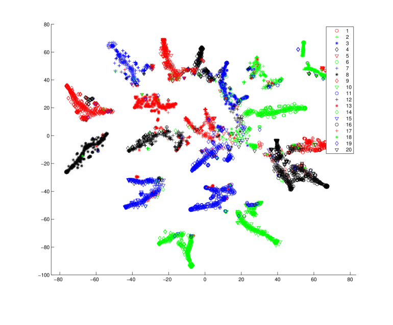
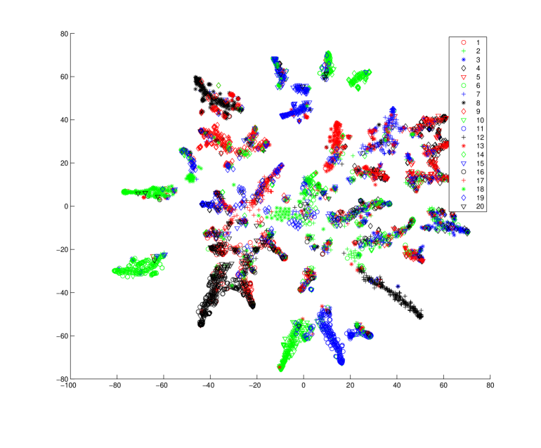
Figure 2: t-SNE 2D embedding of the topic representation by: MedLDA^c (above) and the unsupervised LDA (below).

Class	MedLDA			LDA			Average $\theta$ per class
comp.graphics
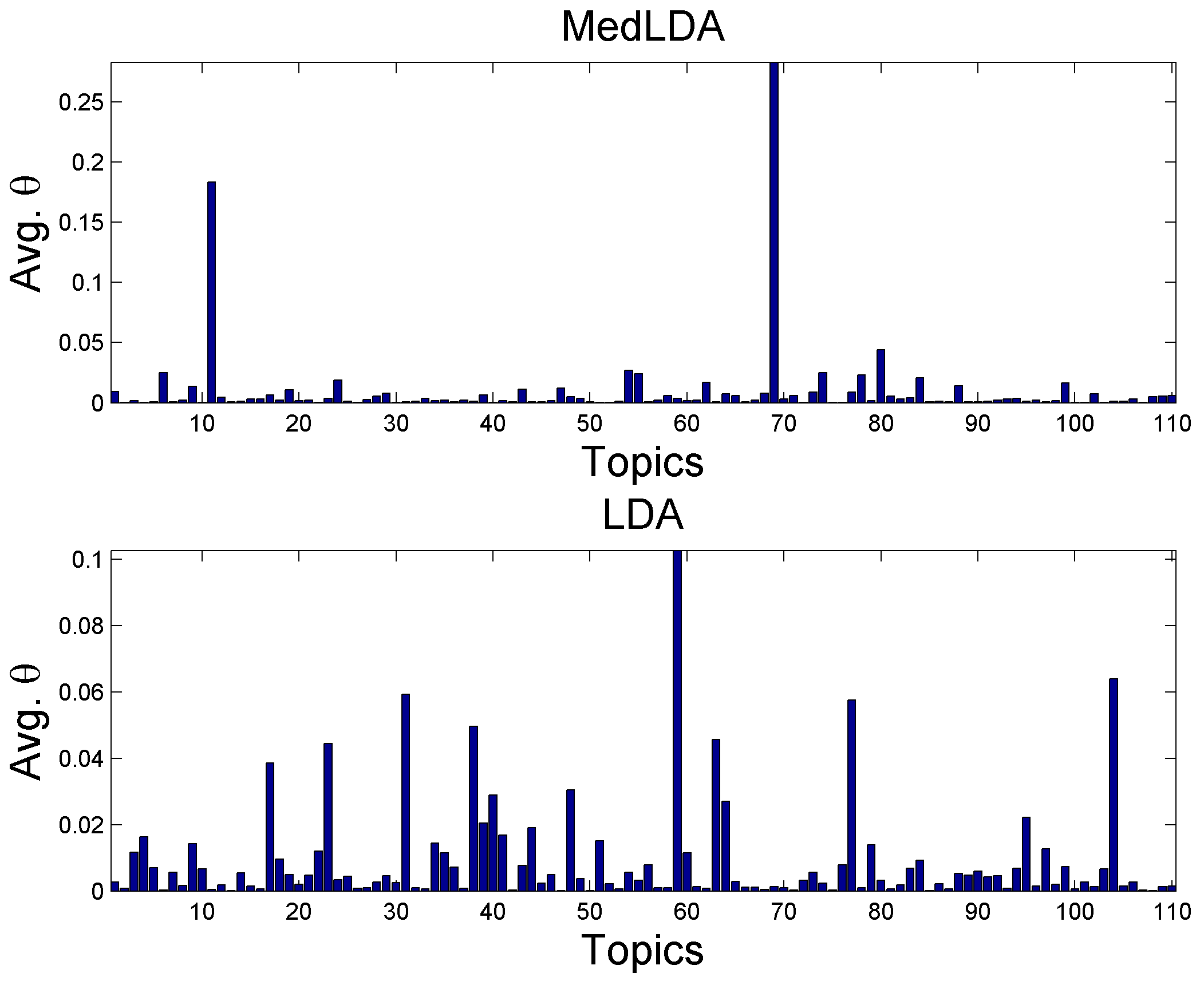
	T $69$	T $11$	T $80$	T $59$	T $104$	T $31$
	image	graphics	db	image	ftp	card
	jpeg	image	key	jpeg	pub	monitor
	gif	data	chip	color	graphics	dos
	file	ftp	encryption	file	mail	video
	color	software	clipper	gif	version	apple
	files	pub	system	images	tar	windows
	bit	mail	government	format	file	drivers
	images	package	keys	bit	information	vga
	format	fax	law	files	send	cards
	program	images	escrow	display	server	graphics
sci.electronics
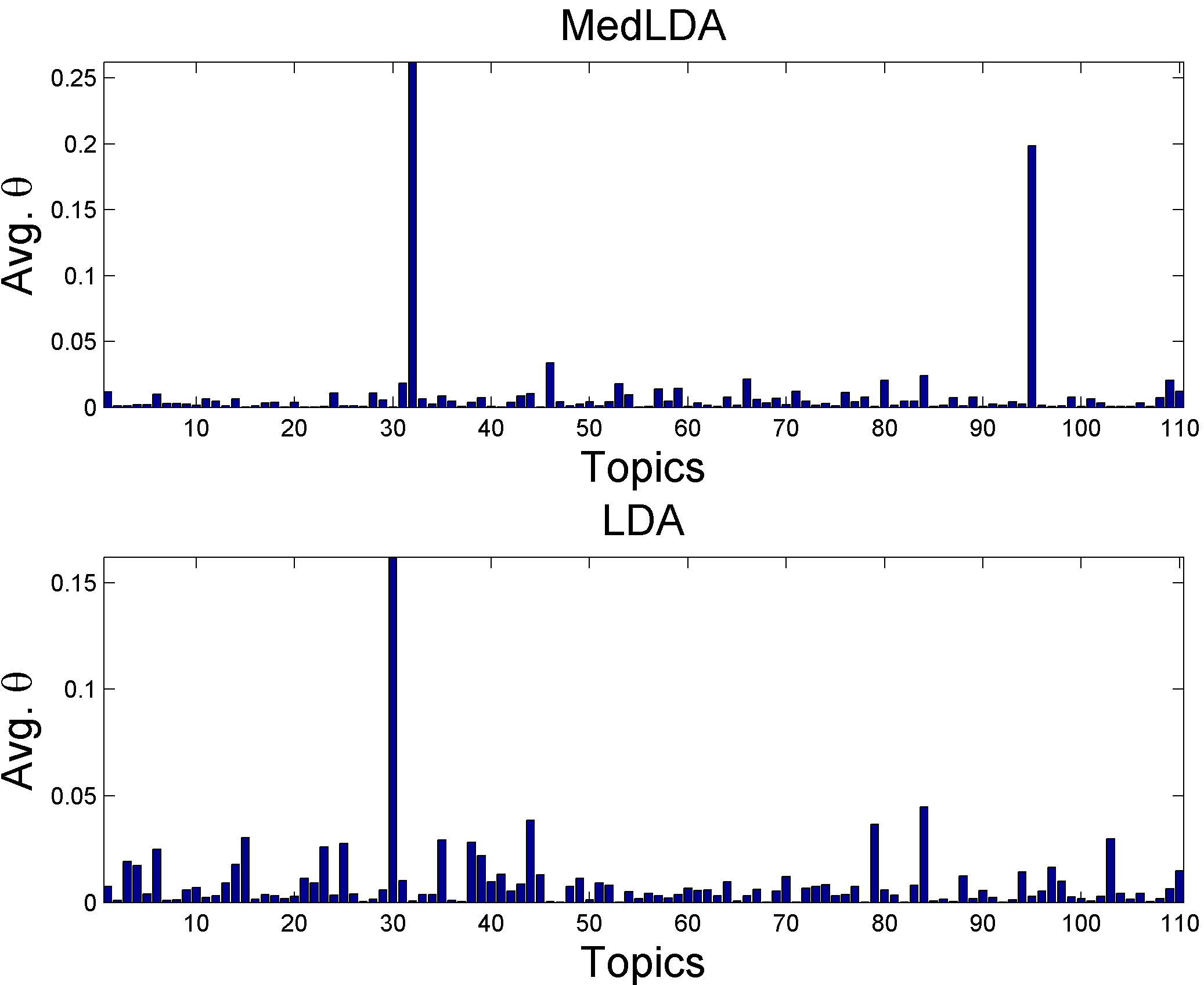
	T $32$	T $95$	T $46$	T $30$	T $84$	T $44$
	ground	audio	source	power	water	sale
	wire	output	rs	ground	energy	price
	power	input	time	wire	air	offer
	wiring	signal	john	circuit	nuclear	shipping
	don	chip	cycle	supply	loop	sell
	current	high	low	voltage	hot	interested
	circuit	data	dixie	current	cold	mail
	neutral	mhz	dog	wiring	cooling	condition
	writes	time	weeks	signal	heat	email
	work	good	face	cable	temperature	cd
politics.mideast
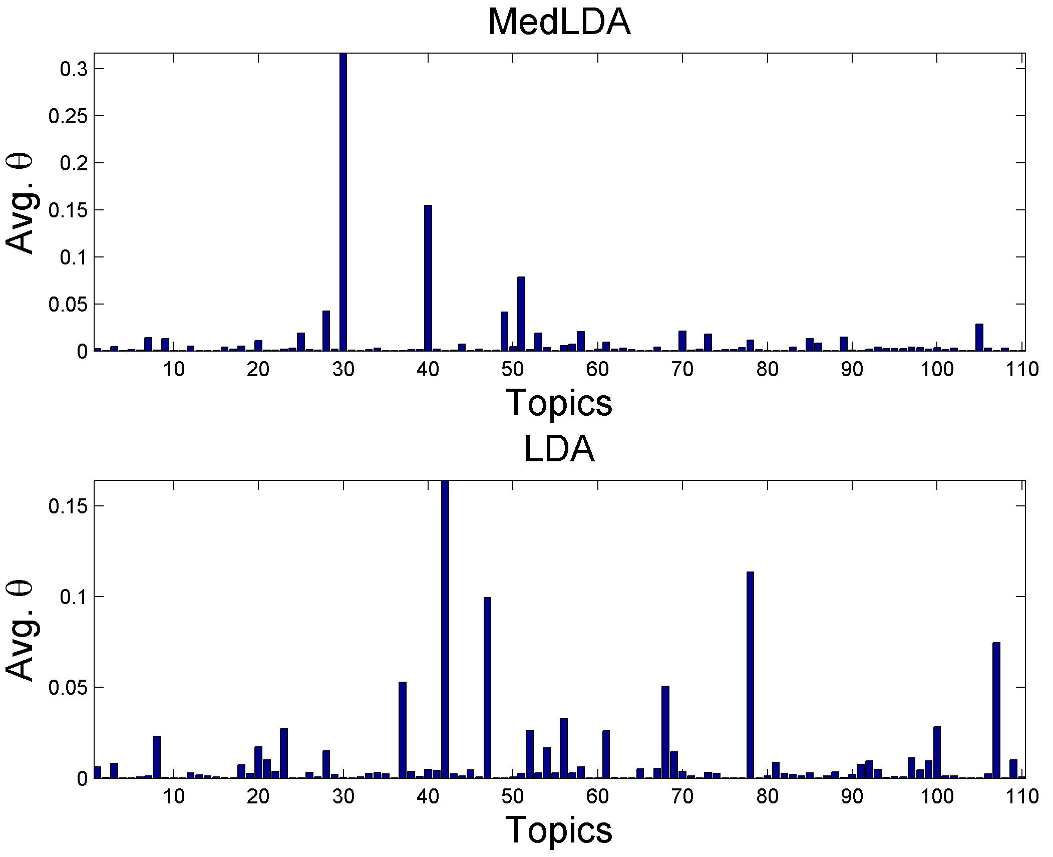
	T $30$	T $40$	T $51$	T $42$	T $78$	T $47$
	israel	turkish	israel	israel	jews	armenian
	israeli	armenian	lebanese	israeli	jewish	turkish
	jews	armenians	israeli	peace	israel	armenians
	arab	armenia	lebanon	writes	israeli	armenia
	writes	people	people	article	arab	turks
	people	turks	attacks	arab	people	genocide
	article	greek	soldiers	war	arabs	russian
	jewish	turkey	villages	lebanese	center	soviet
	state	government	peace	lebanon	jew	people
	rights	soviet	writes	people	nazi	muslim
misc.forsale
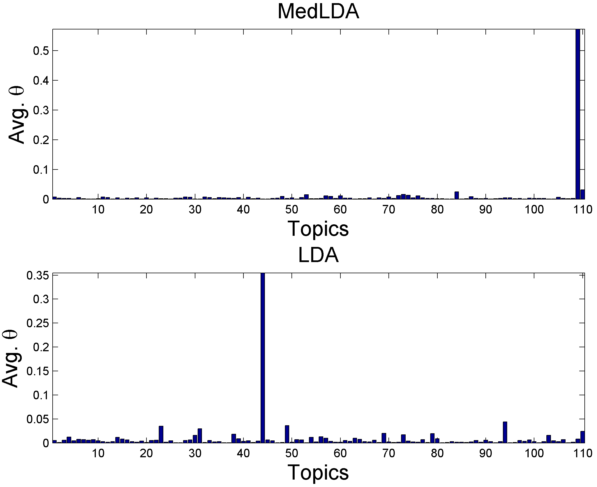
	T $109$	T $110$	T $84$	T $44$	T $94$	T $49$
	sale	drive	mac	sale	don	drive
	price	scsi	apple	price	mail	scsi
	shipping	mb	monitor	offer	call	disk
	offer	drives	bit	shipping	package	hard
	mail	controller	mhz	sell	writes	mb
	condition	disk	card	interested	send	drives
	interested	ide	video	mail	number	ide
	sell	hard	speed	condition	ve	controller
	email	bus	memory	email	hotel	floppy
	dos	system	system	cd	credit	system

Figure 3: Top topics under each class as discovered by the MedLDA and LDA models

We study text modeling of the MedLDA on the 20 Newsgroups data set with a standard list of stop words removed. The data set contains postings in 20 related categories. We compare with the standard unsupervised LDA. We fit the dataset to a 110-topic MedLDA^c model, which explores the supervised category information, and a 110-topic unsupervised LDA.

Figure 2 shows the 2D embedding of the expected topic proportions of MedLDA^c and LDA by using the t-SNE stochastic neighborhood embedding (van der Maaten and Hinton, 2008), where each dot represents a document and color-shape pairs represent class labels. Obviously, the max-margin based MedLDA^c produces a better grouping and separation of the documents in different categories. In contrast, the unsupervised LDA does not produce a well separated embedding, and documents in different categories tend to mix together. A similar embedding was presented in (Lacoste-Jullien et al., 2008), where the transformation matrix in their model is pre-designed. The results of MedLDA^c in Figure 2 are automatically learned.

It is also interesting to examine the discovered topics and their association with class labels. In Figure 3 we show the top topics in four classes as discovered by both MedLDA and LDA. Moreover, we depict the per-class distribution over topics for each model. This distribution is computed by averaging the expected latent representation of the documents in each class. We can see that MedLDA yields sharper, sparser and fast decaying per-class distributions over topics which have a better discrimination power. This behavior is in fact due to the regularization effect enforced over $\phi$ as shown in Eq. (36). On the other hand, LDA seems to discover topics that model the fine details of documents with no regard to their discrimination power (i.e. it discovers different variations of the same topic which results in a flat per-class distribution over topics). For instance, in the class comp.graphics, MedLDA mainly models documents in this class using two salient, discriminative topics (T69 and T11) whereas LDA results in a much flatter distribution. Moreover, in the cases where LDA and MedLDA discover comparably the same set of topics in a given class (like politics.mideast and misc.forsale), MedLDA results in a sharper low dimensional representation.

6.2 Prediction Accuracy

In this subsection, we provide a quantitative evaluation of the MedLDA on prediction performance.

6.2.1 Classification

We perform binary and multi-class classification on the 20 Newsgroup data set. To obtain a baseline, we first fit all the data to an LDA model, and then use the latent representation of the training documents as features to build a binary/multi-class SVM classifier. We denote this baseline by LDA+SVM. For a model $\mathcal{M}$, we evaluate its performance using the relative improvement ratio, i.e., $\frac{precision(\mathcal{M})~{}-~{}precision(LDA+SVM)}{precision(LDA+SVM)}$.

Note that since DiscLDA (Lacoste-Jullien et al., 2008) is using the Gibbs sampling for inference, which is slightly different from the variational methods as in MedLDA and sLDA (Blei and McAuliffe, 2007; Wang et al., 2009), we build the baseline model of LDA+SVM with both variational inference and Gibbs sampling. The relative improvement ratio of each model is computed against the baseline with the same inference method.

Binary Classification: As in (Lacoste-Jullien et al., 2008), the binary classification is to distinguish postings of the newsgroup alt.atheism and the postings of the group talk.religion.misc. We compare MedLDA^c with sLDA, DiscLDA and LDA+SVM. For sLDA, the extension to perform multi-class classification was presented by Wang et al. (2009), we will compare with it in the multi-class classification setting. Here, for binary case, we fit an sLDA regression model using the binary representation (0/1) of the classes, and use a threshold 0.5 to make prediction. For MedLDA^c, to see whether a second-stage max-margin classifier can improve the performance, we also build a method MedLDA+SVM, similar to LDA+SVM. For all the above methods that utilize the class label information, they are fit ONLY on the training data.

We use the SVM-light (Joachims, 1999) to build SVM classifiers and to estimate $q(\eta)$ in MedLDA^c. The parameter $C$ is chosen via 5 fold cross-validation during the training from $\{k^{2}:k=1,\cdots,8\}$. For each model, we run the experiments for 5 times and take the average as the final results. The relative improvement ratios of different models with respect to topic numbers are shown in Figure 4. For the DiscLDA (Lacoste-Jullien et al., 2008), the number of topics is set by the equation $2K_{0}+K_{1}$, where $K_{0}$ is the number of topics per class and $K_{1}$ is the number of topics shared by all categories. As in (Lacoste-Jullien et al., 2008), $K_{1}=2K_{0}$. Here, we set $K_{0}=1,\cdots,8,10$ and align the results with those of MedLDA and sLDA that have the closest topic numbers.

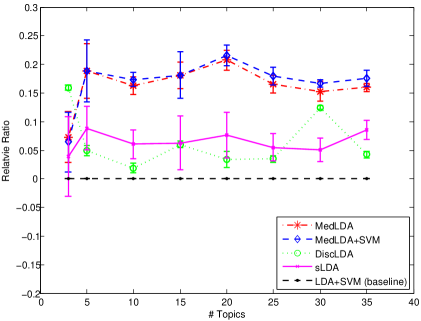
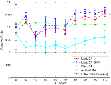
Figure 4: Relative improvement ratio against LDA+SVM for: (a) binary and (b) multi-class classification.

We can see that the max-margin based MedLDA^c works better than sLDA, DiscLDA and the two-step method of LDA+SVM. Since MedLDA^c integrates the max-margin principle in its training, the combination of MedLDA and SVM does not yield additional benefits on this task. We believe that the slight differences between MedLDA and MedLDA+SVM are due to tuning of the regularization parameters. For efficiency, we do not change the regularization constant $C$ during training MedLDA^c. The performance would be improved if we select a good $C$ in different iterations because the data representation is changing.

Multi-class Classification: We perform multi-class classification on 20 Newsgroups with all the categories. We compare MedLDA^c with MedLDA+SVM, LDA+SVM, multi-class sLDA (multi-sLDA) (Wang et al., 2009), and DiscLDA. We use the SVM^struct package with a 0/1 loss to solve the sub-step of learning $q(\eta)$ and build the SVM classifiers for LDA+SVM and MedLDA+SVM. The results are shown in Figure 4. For DiscLDA, we use the same equation as in (Lacoste-Jullien et al., 2008) to set the number of topics and set $K_{0}=1,\cdots,5$. Again, we need to align the results with those of MedLDA based on the closest topic number criterion. We can see that all the supervised topic models discover more predictive topics for classification, and the max-margin based MedLDA^c can achieve significant improvements with an appropriate number (e.g., $\geq 80$) of topics. Again, we believe that the slight difference between MedLDA^c and MedLDA+SVM is due to parameter tuning.

6.2.2 Regression

We evaluate the MedLDA^r model on the movie review data set. As in (Blei and McAuliffe, 2007), we take logs of the response values to make them approximately normal. We compare MedLDA^r with the unsupervised LDA and sLDA. As we have stated, the underlying topic model in MedLDA^r can be a LDA or a sLDA. We have implemented both, as denoted by MedLDA (partial) and MedLDA (full), respectively. For LDA, we use its low dimensional representation of documents as input features to a linear SVR and denote this method by LDA+SVR. The evaluation criterion is predictive R² (pR²) as defined in (Blei and McAuliffe, 2007).

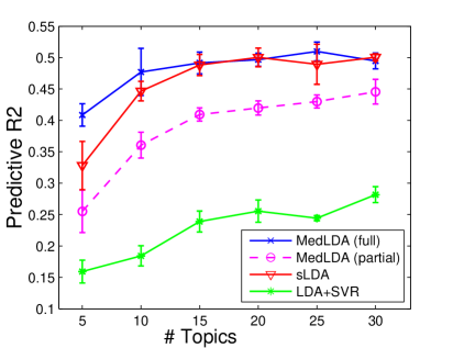
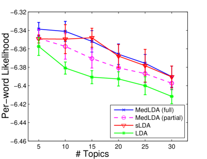
Figure 5: Predictive R² (left) and per-word likelihood (right) of different models on the movie review dataset.

Figure 5 shows the results together with the per-word likelihood. We can see that the supervised MedLDA and sLDA can get much better results than the unsupervised LDA, which ignores supervised responses. By using max-margin learning, MedLDA (full) can get slightly better results than the likelihood-based sLDA, especially when the number of topics is small (e.g., $\leq 15$). Indeed, when the number of topics is small, the latent representation of sLDA alone does not result in a highly separable problem, thus the integration of max-margin training helps in discovering a more discriminative latent representation using the same number of topics. In fact, the number of support vectors (i.e., documents that have at least one non-zero lagrange multiplier) decreases dramatically at $T=15$ and stays nearly the same for $T>15$, which with reference to Eq. (14) explains why the relative improvement over sLDA decreased as $T$ increases. This behavior suggests that MedLDA can discover more predictive latent structures for difficult, non-separable problems.

For the two variants of MedLDA^r, we can see an obvious improvement of MedLDA (full). This is because for MedLDA (partial), the update rule of $\phi$ does not have the third and fourth terms of Eq. (14). Those terms make the max-margin estimation and latent topic discovery attached more tightly. Finally, a linear SVR on the empirical word frequency gets a pR² of 0.458, worse than those of sLDA and MedLDA.

6.2.3 Time Efficiency

For binary classification, MedLDA^c is much more efficient than sLDA, and is comparable with the LDA+SVM, as shown in Figure LABEL:fig:time. The slowness of sLDA may be due to the mismatching between its normal assumption and the non-Gaussian binary response variables, which prolongs the E-step. For multi-class classification, the training time of MedLDA^c is mainly dependent on solving a multi-class SVM problem, and thus is comparable to that of LDA. For regression, the training time of MedLDA (full) is comparable to that of sLDA, while MedLDA (partial) is more efficient.

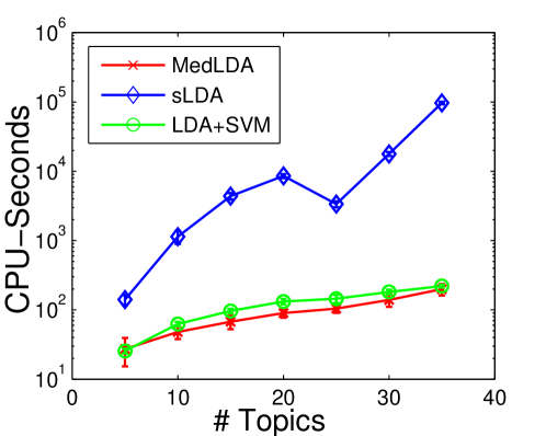
Figure 6: Training time of different models with respect to the number of topics for binary classification.

7 Related Work

Latent Dirichlet Allocation (LDA) (Blei et al., 2003) is a hierarchical Bayesian model for discovering latent topics in a document collection. LDA has found wide applications in information retrieval, data mining, computer vision, and etc. The LDA is an unsupervised model.

Supervised LDA (Blei and McAuliffe, 2007) was proposed for regression problem. Although the sLDA was generalized to classification with a generalized linear model (GLM), no results have been reported on the classification performance of sLDA. One important issue that hinders the sLDA to be effectively applied for classification is that it has a normalization factor because sLDA defines a fully generative model. The normalization factor makes the learning very difficult, where variatioinal method or higher-order statistics must be applied to deal with the normalizer, as shown in (Blei and McAuliffe, 2007). Instead, MedLDA applies the concept of margin and directly concentrates on maximizing the margin. Thus, MedLDA does not need to define a fully generative model, and the problem of MedLDA for classification can be easily handled via solving a dual QP problem, in the same spirit of SVM.

DiscLDA (Lacoste-Jullien et al., 2008) is another supervised LDA model, which was specifically proposed for classification problem. DiscLDA also defines a fully generative model, but instead of minimizing the evidence, it minimizes the conditional likelihood, in the same spirit of conditional random fields (Lafferty et al., 2001). Our MedLDA significantly differs from the DiscLDA. The implementation of MedLDA is extremely simple.

Other variants of topic models that leverage supervised information have been developed in different application scenarios, including the models for online reviews (Titov and McDonald, 2008; Branavan et al., 2008), image annotation (He and Zemel, 2008) and the credit attribution Labeled LDA model (Ramage et al., 2009).

Maximum entropy discrimination (MED) (Jaakkola et al., 1999) principe provides an excellent combination of max-margin learning and Bayesian-style estimation. Recent work (Zhu et al., 2008b) extends the MED framework to the structured learning setting and generalize to incorporate structured hidden variables in a Markov network. MedLDA is an application of the MED principle to learn a latent Dirichlet allocation model. Unlike (Westerdijk and Wiegerinck, 2000), where a generative model is degenerated to a deterministic version for classification, our model is generative and thus can discover the latent topics over document collections.

The basic principle of MedLDA can be generalized to the structured prediction setting, in which multi-variant response variables are predicted simultaneously and thus their mutual dependencies can be explored to achieve globally consistent and optimal predictions. At least two scenarios are within our horizon that can be directly solved via MedLDA, i.e., the image annotation (He and Zemel, 2008), where neighboring annotation tends to be smooth, and the statistical machine translation (Zhao and Xing, 2006), where tokens are naturally aligned in word sentences.

8 Conclusions and Discussions

We have presented the maximum entropy discrimination LDA (MedLDA) that uses the max-margin principle to train supervised topic models. MedLDA integrates the max-margin principle into the latent topic discovery process via optimizing one single objective function with a set of expected margin constraints. This integration yields a predictive topic representation that is more suitable for regression or classification. We develop efficient variational methods for MedLDA. The empirical results on movie review and 20 Newsgroups data sets show the promise of MedLDA on text modeling and prediction accuracy.

MedLDA represents the first step towards integrating the max-margin principle into supervised topic models, and under the general MedTM framework presented in Section 3, several improvements and extensions are in the horizon. Specifically, due to the nature of MedTM’s joint optimization formulation, advances in either max-margin training or better variational bounds for inference can be easily incorporated. For instance, the mean field variational upper bound in MedLDA can be improved by using the tighter collapsed variational bound (Teh et al., 2006) that achieves results comparable to collapsed Gibbs sampling (Griffiths and Steyvers, 2004). Moreover, as the experimental results suggest, incorporation of a more expressive underlying topic model enhances the overall performance. Therefore, we plan to integrate and utilize other underlying topic models like the fully generative sLDA model in the classification case. Finally, advanced in max-margin training would also results in more efficient training.

Proof of Corollary 3

In this section, we prove the corollary 3.

Proof  Since the variational parameters $(\gamma,\phi)$ are fixed when solving for $q(\eta)$, we can ignore the terms in $\mathcal{L}^{bs}$ that do not depend on $q(\eta)$ and get the function

$$\mathcal{L}^{bs}_{[q(\eta)]} \triangleq KL(q(\eta)\|p_{0}(\eta))-\sum_{d}E_{q}[\log p(y_{d}|\bar{Z}_{d},\eta,\delta^{2})]$$

$$=KL(q(\eta)\|p_{0}(\eta))+\frac{1}{2\delta^{2}}\Big{(}E_{q(\eta)}\big{[}\eta^{\top}E[AA^{\top}]\eta-2\eta^{\top}\sum_{d=1}^{D}y_{d}E[\bar{Z}_{d}]\big{]}\Big{)}+c,$$

where $c$ is a constant that does not depend on $q(\eta)$.

Let $U(\xi,\xi^{\star})=C\sum_{d=1}^{D}(\xi_{d}+\xi_{d}^{\star})$. Suppose $(q_{0}(\eta),\xi_{0},\xi_{0}^{\star})$ is the optimal solution of P1, then we have: for any feasible $(q(\eta),\xi,\xi^{\star})$,

$$\mathcal{L}^{bs}_{[q_{0}(\eta)]}+U(\xi_{0},\xi_{0}^{\star})\leq\mathcal{L}^{bs}_{[q(\eta)]}+U(\xi,\xi^{\star}).$$

From Corollary 2, we conclude that the optimum predictive parameter distribution is $q_{0}(\eta)=\mathcal{N}(\lambda_{0},\Sigma)$, where $\Sigma=(I+1/\delta^{2}E[A^{\top}A])^{-1}$ does not depend on $q(\eta)$. Since $q_{0}(\eta)$ is also normal, for any distribution $q(\eta)=\mathcal{N}(\lambda,\Sigma)$, with several steps of algebra it is easy to show that

$$\mathcal{L}^{bs}_{[q(\eta)]}=\frac{1}{2}\lambda^{\top}(I+\frac{1}{\delta^{2}}E[A^{\top}A])\lambda-\lambda^{\top}(\sum_{d=1}^{D}\frac{y_{d}}{\delta^{2}}E[\bar{Z}_{d}])+c^{\prime}=\frac{1}{2}\lambda^{\top}\Sigma^{-1}\lambda-\lambda^{\top}(\sum_{d=1}^{D}\frac{y_{d}}{\delta^{2}}E[\bar{Z}_{d}])+c^{\prime},$$

where $c^{\prime}$ is another constant that does not depend on $\lambda$.

Thus, we can get: for any $(\lambda,\xi,\xi^{\star})$, where

$$(\lambda,\xi,\xi^{\star})\in\{(\lambda,\xi,\xi^{\star}):~{}y_{d}-\lambda^{\top}E[\bar{Z}_{d}]\leq\epsilon+\xi_{d};~{}-y_{d}+\lambda^{\top}E[\bar{Z}_{d}]\leq\epsilon+\xi_{d}^{\star};~{}\textrm{and}~{}\xi,\xi^{\star}\geq 0~{}\forall d\},$$

we have

$$\frac{1}{2}\lambda_{0}^{\top}\Sigma^{-1}\lambda_{0}-\lambda_{0}^{\top}(\sum_{d=1}^{D}\frac{y_{d}}{\delta^{2}}E[\bar{Z}_{d}])+U(\xi_{0},\xi_{0}^{\star})\leq\frac{1}{2}\lambda^{\top}\Sigma^{-1}\lambda-\lambda^{\top}(\sum_{d=1}^{D}\frac{y_{d}}{\delta^{2}}E[\bar{Z}_{d}])+U(\xi,\xi^{\star}),$$

which means the mean of the optimum posterior distribution under a Gaussian MedLDA is achieved by solving a primal problem as stated in the Corollary.

References

- Blei and Lafferty [2005] David Blei and John Lafferty. Correlated topic models. In Advances in Neural Information Processing Systems (NIPS), 2005.
- Blei and McAuliffe [2007] David Blei and Jon D. McAuliffe. Supervised topic models. In Advances in Neural Information Processing Systems (NIPS), 2007.
- Blei et al. [2003] David Blei, Andrew Ng, and Michael Jordan. Latent Dirichlet allocation. Journal of Machine Learning Research, (3):993–1022, 2003.
- Branavan et al. [2008] S.R.K. Branavan, Harr Chen, Jacob Eisenstein, and Regina Barzilay. Learning document-level semantic properties from free-text annotations. In Proceddings of the Annual Meeting of the Association for Computational Linguistics (ACL), 2008.
- Chechik and Tishby [2002] Gal Chechik and Naftali Tishby. Extracting relevant structures with side information. In Advances in Neural Information Processing Systems (NIPS), 2002.
- Crammer and Singer [2001] Koby Crammer and Yoram Singer. On the algorithmic implementation of multiclass kernel-based vector machines. Journal of Machine Learning Research, (2):265–292, 2001.
- Griffiths and Steyvers [2004] T. Griffiths and M. Steyvers. Finding scientific topics. Proceedings of the National Academy of Sciences, (101):5228–5235, 2004.
- He and Zemel [2008] Xuming He and Richard S. Zemel. Learning hybrid models for image annotation with partially labeled data. In Advances in Neural Information Processing Systems (NIPS), 2008.
- Jaakkola et al. [1999] Tommi Jaakkola, Marina Meila, and Tony Jebara. Maximum entropy discrimination. In Advances in Neural Information Processing Systems (NIPS), 1999.
- Joachims [1999] Thorsten Joachims. Making large-scale SVM learning practical. Advances in kernel methods–support vector learning, MIT-Press, 1999.
- Jordan et al. [1999] Michael I. Jordan, Zoubin Ghahramani, Tommis Jaakkola, and Lawrence K. Saul. An introduction to variational methods for graphical models. M. I. Jordan (Ed.), Learning in Graphical Models, Cambridge: MIT Press, Cambridge, MA, 1999.
- Lacoste-Jullien et al. [2008] Simon Lacoste-Jullien, Fei Sha, and Michael I. Jordan. DiscLDA: Discriminative learning for dimensionality reduction and classification. In Advances in Neural Information Processing Systems (NIPS), 2008.
- Lafferty et al. [2001] John Lafferty, Andrew McCallum, and Fernando Pereira. Conditional random fields: Probabilistic models for segmenting and labeling sequence data. In ICML, 2001.
- Pavlov et al. [2003] Dmitry Pavlov, Alexandrin Popescul, David M. Pennock, and Lyle H. Ungar. Mixtures of conditional maximum entropy models. In ICML, 2003.
- Ramage et al. [2009] Daniel Ramage, David Hall, Ramesh Nallapati, and Christopher D. Manning. Labeled lda: A supervised topic model for credit attribution in multi-labeled corpora. In Proceddings of the 2009 Conference on Empirical Methods in Natural Language Processing, 2009.
- Russell et al. [2008] Bryan C. Russell, Antonio Torralba, Kevin P. Murphy, and William T. Freeman. Labelme: a database and web-based tool for image annotation. International Journal of Computer Vision, 77(1-3):157–173, 2008.
- Smola and Schlkopf [2003] Alex J. Smola and Bernhard Schlkopf. A tutorial on support vector regression. Statistics and Computing, 2003.
- Teh et al. [2006] Yee Whye Teh, David Newman, and Max Welling. A collapsed variational bayesian inference algorithm for latent dirichlet allocation. In Advances in Neural Information Processing Systems (NIPS), 2006.
- Titov and McDonald [2008] Ivan Titov and Ryan McDonald. A joint model of text and aspect ratings for sentiment summarization. In Proceddings of the Annual Meeting of the Association for Computational Linguistics (ACL), 2008.
- van der Maaten and Hinton [2008] L.J.P. van der Maaten and G.E. Hinton. Visualizing data using t-SNE. Journal of Machine Learning Research, (9):2579–2605, 2008.
- Vapnik [1995] V. Vapnik. The Nature of Statistical Learning Theory. Springer, New York, 1995.
- Wang et al. [2009] Chong Wang, David Blei, and Fei-Fei Li. Simultaneous image classification and annotation. In IEEE Computer Society Conference on Computer Vision and Pattern Recognition, 2009.
- Welling et al. [2004] Max Welling, Michal Rosen-Zvi, and Geoffrey Hinton. Exponential family harmoniums with an application to information retrieval. In Advances in Neural Information Processing Systems (NIPS), 2004.
- Westerdijk and Wiegerinck [2000] Michael Westerdijk and Wim Wiegerinck. Classification with multiple latent variable models using maximum entropy discrimination. In ICML, 2000.
- Yang et al. [2007] Jun Yang, Yan Liu, Eric P. Xing, and Alexander G. Hauptmann. Harmonium models for semantic video representation and classification. In SIAM Conf. on Data Mining, 2007.
- Zhao and Xing [2006] Bin Zhao and Eric P. Xing. Hm-bitam: Bilingual topic exploration, word alignment, and translation. In Advances in Neural Information Processing Systems (NIPS), 2006.
- Zhu et al. [2008a] Jun Zhu, Eric P. Xing, and Bo Zhang. Laplace maximum margin Markov networks. In International Conference on Machine Learning, 2008a.
- Zhu et al. [2008b] Jun Zhu, Eric P. Xing, and Bo Zhang. Partially observed maximum entropy discrimination Markov networks. In Advances in Neural Information Processing Systems (NIPS), 2008b.