Self-consistent modeling of pair cascades in the polar cap of a pulsar.
Abstract
Here we briefly report on first results of self-consistent simulation of non-stationary electron-positron cascades in the polar cap of pulsar using specially developed hybrid PIC/Monte-Carlo numerical code. We consider the case of Ruderman-Sutherland cascade – when particles cannot be extracted from the surface of the neutrons star.
I INTRODUCTION
Many previously proposed models for polar cap cascades (and almost all quantitative models) assumed stationary particle outflow (Arons and Scharlemann, 1979; Daugherty and Harding, 1982; Muslimov and Tsygan, 1992; Harding and Muslimov, 2002; Hibschman and Arons, 2001). Predictions of such models disagree with both observational data (e.g. the number of electron-positron pairs in pulsar wind nebula is much higher than predicted, e.g. (de Jager, 2007)) and results of numerical models of force-free pulsar magnetosphere (the current density required to support force-free magnetosphere differs substantially from what stationary model for polar cap cascade predicts (Timokhin, 2006)). On the other hand, the stability of such stationary models has not been quantitatively studied.
Particle acceleration and electron-positron pair production in the polar cap could be essentially non-stationary: time intervals of effective particle acceleration could alternate with intervals when the accelerating electric field is screened by electron-positron pairs created in the cap (Sturrock, 1971; Al’Ber et al., 1975; Ruderman and Sutherland, 1975; Levinson et al., 2005). To construct a consistent model for particle acceleration in the polar cap and high energy emission produced there we need to know the pattern of particle flow. In our view, the study of electron-positron cascades should be done starting ab initio. The key “ingredients” of the system must be included in the model: back reaction of particles on the accelerating electric field and the delay between photon emission and pair injection. Possible complexity of the system behavior compels us to conduct a numerical experiment where particle acceleration, pair production and variation in the accelerating electric field are modeled self-consistently.
Here we presents first results of such self-consistent modeling. We consider the case of Ruderman-Sutherland cascade and describe the main properties of the discharge.
II NUMERICAL METHOD
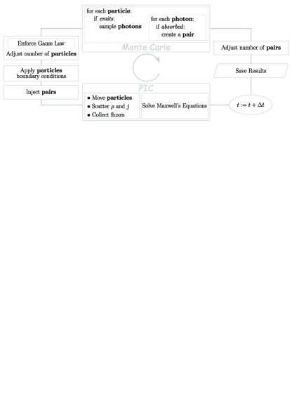
For modeling of pair cascades we developed special hybrid PIC/Monte Carlo code. Current version of the code is 1D. The code flow schematic is shown in Fig. 1, the code works as follows.
Plasma dynamics is calculated according to the standard PIC algorithm. Using the current density known from the previous step we solve Maxwell equations and get the electric field at the grid points. Then for each particle we interpolate the electric field to the particle’s position and get the force on the particle. By solving the equation of motion we advance particle’s momentum and position. Motion of particles across cell boundaries is counted as their contribution to the electric current which is collected and stored for the next time step.
Photon emission and pair production are calculated as follows. We sample how many photons capable of producing electron-positron pairs each particle emits during the current time step. For each emitted photon we sample its energy from the energy distribution for a given emission process. Then we sample the distance which the photon will travel until it gets absorbed. Calculation of the optical depth to pair creation is done with space steps varying according to the current value of the cross-section for photon absorption. Most of the steps are much larger that the cell size. The energy of the photon, the position and the time of the absorption are stored in an array. At every time step we iterate over that array and pick up photons which must be absorbed at the time of the current time step. For each of the selected photons we inject an electron and a positron at the place of the absorption and delete that photon from the array. Being injected at the same point, the electron and the positron do not change charge and current densities at the moment of injection.
If there are too many numerical particles of some kind in the computational domain, their number can be reduced by deleting some randomly selected particles. Statistical weights of the selected particles are summed and then the statistical weights of all remaining particles of the same kind as deleted ones are increased correspondingly in order to compensate for the deleted particles.
III PHYSICAL MODEL
As previously there were no direct self-consistent kinetic studies of time depended cascade starting from the first principles, we decided to address first a simple case in order to develop an intuition of what kind of plasma behavior to expect and to adjust the numerical technique accordingly. Ruderman and Sutherland (1975) cascade is the simplest possible model for the pair cascade in the polar cap – there is no plasma inflow from the surface of the neutron star (NS) and all plasma in the cascade zone is produced by pair creation.
Ruderman and Sutherland (1975) estimate for the height of the cascade zone for young pulsars (their eq. (22)) gives
| (1) |
For young pulsars, with periods less than sec, is less that the width of the polar cap cm. Therefore, one-dimensional approximation should work well for such cascades. In 1D the continuity equation for the charge density and the Gauss equation for the accelerating electric field can be combined into the single equation for the electric field (see e.g. (Levinson et al., 2005))
| (2) |
where is the actual current density and is the mean current density flowing through the system. This is the equation we solve for the electric field. It does not need explicitly set boundary conditions on . Boundary conditions are implicitly set by the choice of . The initial electric field distribution is calculated as solution of 1D Gauss equation for some given initial charge density distribution and initial boundary conditions.
For young pulsars the dominating emission process in terms of number of pair-production capable photons is the curvature radiation (e.g. (Hibschman and Arons, 2001)). We are primarily interested in the dynamics of the discharge zone (the region with the accelerating electric field). The size of that zone should be of the order of few . Synchrotron photons emitted by electron-positron pairs are much less energetic than the curvature photons and, therefore, these photons have much larger mean free paths. They are absorbed at large distances from the NS, where plasma density is expected to be very high and electric field is already screened. Consecutively, pairs produced by the synchrotron photons do not influence the discharge dynamics and we ignore synchrotron emission in our simulations.
So, our model for the Ruderman-Sutherland cascade includes 1D electrodynamics, curvature radiation as the photon emission process, photon absorption and pair creation in strong magnetic field. Particle equation of motion includes radiation reaction due to curvature radiation.
IV RESULTS OF NUMERICAL SIMULATIONS
Numerical simulation have shown that in the Ruderman-Sutherland model pair creation is quasi-periodic and self-sustained. We performed simulations for different initial particle distributions and different initial electric fields, different strengths of the magnetic field, different radii of curvature of magnetic field lines and for different pulsar periods. After the initial burst of pair creation the cascade zone always settled down to a quasi-periodic behavior qualitatively similar for all physical parameters admitting pair creation. The system seems to forget initial conditions and after a short relaxation (couple of flyby times) for given magnetic field, pulsar period and the mean current its behavior is the same independent on the initial configuration.
We describe here main properties of the cascade using as an example the case with the mean current density equal to the Goldreich-Julian (Goldreich and Julian, 1969) current density, . For the mean current density different from cascade behavior is qualitatively similar. In this example we consider a pulsar with period sec, magnetic field G, radius of curvature of the magnetic field lines cm (such value for was used in (Ruderman and Sutherland, 1975)). We performed simulations for pure dipole magnetic field with cm too. Qualitatively results do not depend on the radius of curvature, but for smaller calculations with the same numerical resolution can be done faster, as the size of the gap with accelerating electric field is smaller. Angular velocity of NS rotation is anti-parallel to the magnetic moment of the star, so the Goldreich-Julian change density is positive.
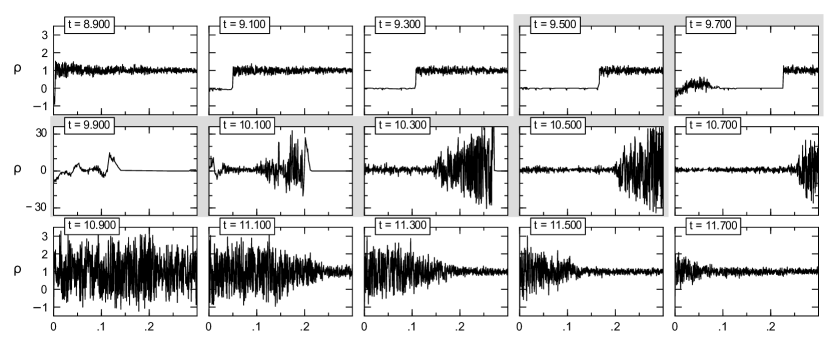
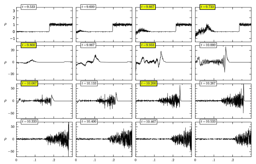
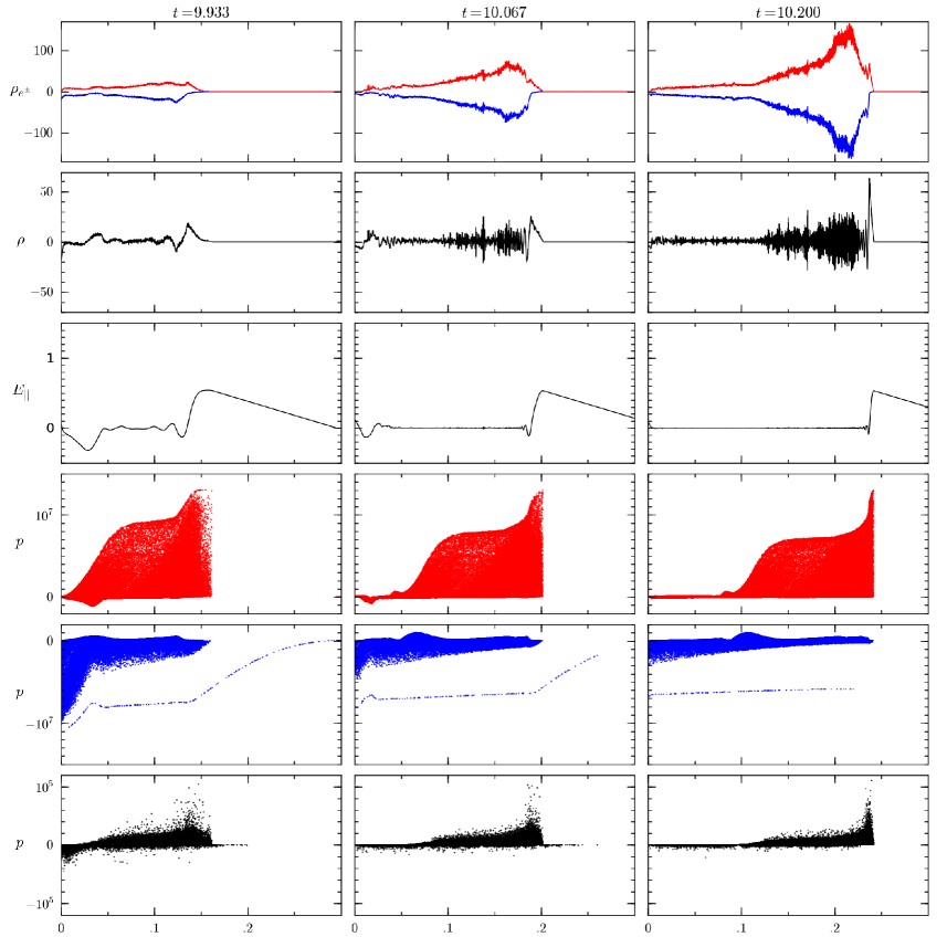
We describe below a whole cycle of pair formation and illustrate the cascade development by a series of snapshots at several time moments during one cycle with plots showing different physical quantities in Figs. 2, 3, 4. In these figures we present plots for a typical cycle of pair formation taken from a long simulation where several such cycles were observed. The time on this figures is normalized to the flyby time of the computational domain. Time is counted from the start of a particular simulation, so its absolute value has no physical meaning – only time intervals between the shots have physical meaning.
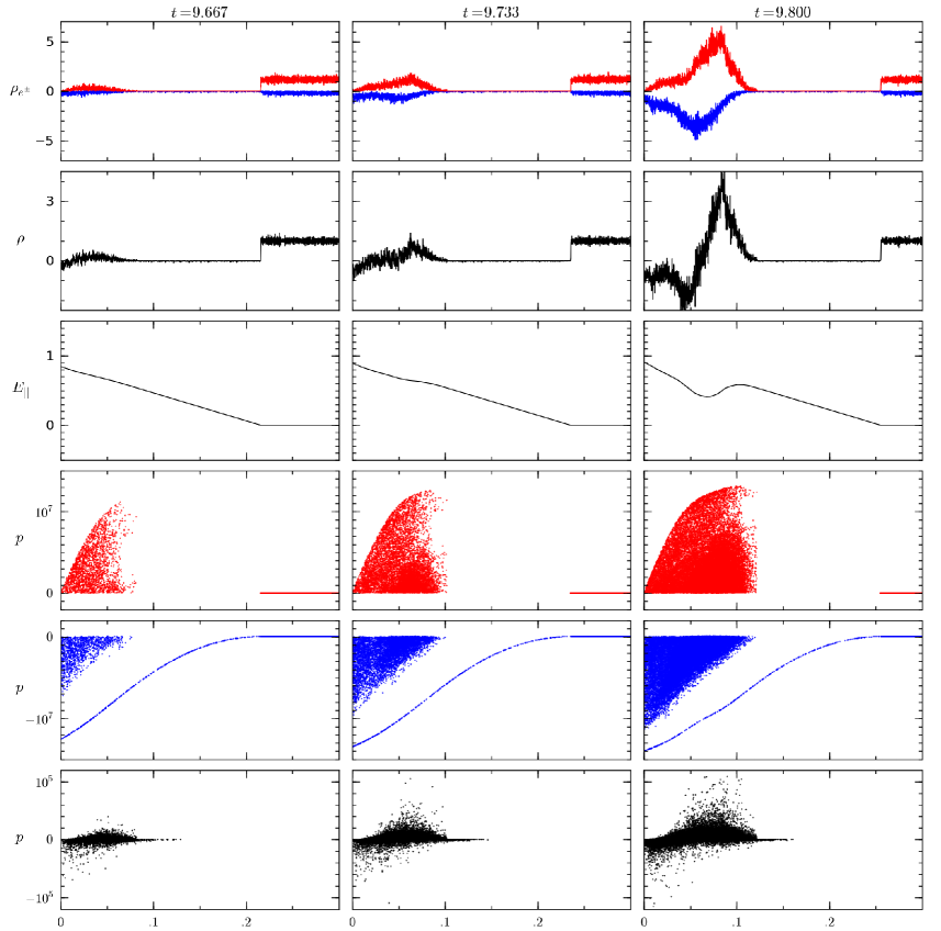
Changes in the charge density distribution gives the best overview of what is going on in the discharge zone, because charge density indirectly provides information about both the particle number density and the electric field. In Fig. 2 we plot the change density at equally spaced time interval during the discharge cycle. In the upper panel of that figure we present an overview of the entire cycle, in the lower panel we plot snapshots of the change density distribution at smaller time intervals for the most interesting part of the discharge – formation of a new plasma blob. In Figs. 3, 4 we show more detailed information about physical conditions in the discharge zone: the number densities of electrons and positron, the accelerating electric field, phase portraits of electrons, positrons and pair producing photons. On the phase portraits particles with positive values of the 4-momentum are those which move from the NS, particles with negative move toward the NS.
A typical cycle of the discharge starts with a vacuum gap forming above the surface of the NS (snapshots with ). The electric field there is very strong and charged particles entering the gap are accelerated up to very high energies. Plasma creation starts close to the NS and is ignited by the gamma-rays emitted by electrons flowing toward the NS. These “primary” electrons have been created in the previous bursts of pair formation. They leaks from the tail of the plasma blob created in the previous cycle and enters the gap from above. The newly created electrons and positrons are accelerated by the strong electric field of the gap and start producing high energy photons, many of which decay into pairs too (snapshot with in Figs. 3, 2). In Fig. 3, 4 on the plots showing the phase portrait for electrons “primary” electrons accelerated in the gap can be seen as the particle population having thin line-like form. Particle populations scattered over the large area beginning at the left end of the phase space plots represent secondary particles.
While number density of the pair plasma remains less then the Goldreich-Julian density, the electric field remains strong and electrons and positrons are accelerated to energies high enough to emit photons capable of producing pairs (see snapshots with ). When the number density become larger than the Goldreich-Julian density, acceleration of particles ceases and particles created after that moment do not emit pair-producing photons. Screening of the electric field begins near the NS surface, where first pairs are formed, so the region of a very low plasma density (the gap) with strong electric field detaches from the NS surface and propagates into the magnetosphere (snapshots with ). From below this gap is limited by the blob of freshly formed plasma, from above – by the plasma created in the previous burst of pair formation. Particles from the previous bursts of pair formation which have momentum directed toward the NS enters the gap from above. Electrons are accelerated toward the NS, positrons are turned back by the strong electric field of the gap and move into the magnetosphere. Because of this reversal the gap upper boundary moves noticeably slower than the speed of light. The front of the blob with the freshly created plasma consists of ultra-relativistic positrons accelerated in then strong electric field, so it moves relativistically and, therefore, the gap shrinks when the blob moves into the magnetosphere. Pairs are continuously injected into the blob, because it practically co-moves with the pair-producing photons. Eventually the front of the new blob catches the tail of the previously created blob. Therefore, the magnetosphere will be filled with plasma and there will be no gaps in plasma spacial distribution far from the polar cap. When the blob has traveled some distance a new gap starts forming, ignited by the electrons leaving the current blob.
When the electric field is still strong large amplitude plasma oscillations are excited in the newly formed plasma. These oscillations persists after the global accelerating field has been screened. Fluctuating electric field of the oscillations reverses some electrons and positrons toward the NS. These particles forms the above mentioned tail of the plasma blob. The electrons from that tail will be the “primary” particles in the next burst of pair formation.
V Conclusions and open issues
Main findings from the numerical simulations can be summarized as follows. The Ruderman-Sutherland cascade can operate for any positive current density. The cascade is self-sustained and discharges occur quasi-periodically, the whole systems shows a sort of limit cycle behavior. As cascade properties do not depend on the initial conditions in our simulations, they are uniquely set by the mean current density , the potential drop across the polar cap and the curvature of the magnetic field lines. Distribution of the pair plasma in the magnetosphere is continuous, with no gaps, so the parallel component of the electric field far from the polar cap should be screened. Thus, such cascade model agrees well with force-free magnetosphere models (e.g. Contopoulos et al., 1999; Timokhin, 2006; Spitkovsky, 2006). Strong plasma oscillations are excited in the plasma blob during its formation. This might have implication for generation of radioemission.
While the general structure of the flow is evident from the performed simulations, some questions remain unanswered. The most important one is about the period of these discharge. It depends on the rate of plasma leakage from the blob, i.e. how many particles are reversed toward the NS. The more particles leaks out, the later the next gap forms. Due to continuous pair injection plasma density in the blob increases enormously, and at some time the numerical scheme stops resolving the Debye length of the plasma, and the damping of the plasma oscillations cannot be calculated reliably. At that time results start depending on the numerical resolution. Because of this the blob cannot be followed for time interval long enough (and traveled distances large enough) to get the repetition rate of the cascade. In the presented simulations the size of the simulation zone is set such that the blob leaves calculation domain before the numerical scheme fails to model it correctly. So, while particle energy distribution can be inferred from current simulations, pair multiplicity and particle fluxes are known up to some numerical factor which depends on the repetition rate of pair creation bursts.
More detailed description of the results as well as discussion of their implication for pulsar physics will be given in a subsequent publication.
Acknowledgements.
I’m deeply indebted to Jonathan Arons for encouragement, continuous support, and for innumerable exciting discussions which substantially influenced my understanding of the problem. This work was supported by NSF grant AST-0507813 and NASA grants NNG06GJI08G and NNX09AU05G.References
- Arons and Scharlemann (1979) J. Arons and E. T. Scharlemann, Astrophys. J. 231, 854 (1979).
- Daugherty and Harding (1982) J. K. Daugherty and A. K. Harding, Astrophys. J. 252, 337 (1982).
- Muslimov and Tsygan (1992) A. G. Muslimov and A. I. Tsygan, MNRAS 255, 61 (1992).
- Harding and Muslimov (2002) A. K. Harding and A. G. Muslimov, Astrophys. J. 568, 862 (2002).
- Hibschman and Arons (2001) J. A. Hibschman and J. Arons, Astrophys. J. 554, 624 (2001).
- de Jager (2007) O. C. de Jager, Astrophys. J. 658, 1177 (2007).
- Timokhin (2006) A. N. Timokhin, MNRAS 368, 1055 (2006).
- Ruderman and Sutherland (1975) M. A. Ruderman and P. G. Sutherland, Astrophys. J. 196, 51 (1975).
- Sturrock (1971) P. A. Sturrock, Astrophys. J. 164, 529 (1971).
- Al’Ber et al. (1975) Y. I. Al’Ber, Z. N. Krotova, and V. Y. Eidman, Astrophysics 11, 189 (1975).
- Levinson et al. (2005) A. Levinson, D. Melrose, A. Judge, and Q. Luo, Astrophys. J. 631, 456 (2005).
- Goldreich and Julian (1969) P. Goldreich and W. H. Julian, Astrophys. J. 157, 869 (1969).
- Contopoulos et al. (1999) I. Contopoulos, D. Kazanas, and C. Fendt, Astrophys. J. 511, 351 (1999).
- Spitkovsky (2006) A. Spitkovsky, ApJ Letters 648, L51 (2006).