We develop a variable depth search heuristic for the quadratic assignment problem. The heuristic is based on sequential changes in assignments analogous to the Lin-Kernighan sequential edge moves for the traveling salesman problem. We treat unstructured problem instances of sizes 60 to 400. When the heuristic is used in conjunction with robust tabu search, we measure performance improvements of up to a factor of 15 compared to the use of robust tabu alone. The performance improvement increases as the problem size increases.

Key words: combinatorics; quadratic assignment problem; hybrid heuristic; variable depth sequential search

History:

1 Introduction

The quadratic assignment problem (QAP) is a combinatorial optimization problem first introduced by Koopmans and Beckman (1957). It is NP-hard and is considered to be one of the most difficult problems to be be solved optimally. The problem was defined in the following context: A set of $N$ facilities are to be located at $N$ locations. The distance between locations $i$ and $j$ is $D(i,j)$ and the quantity of materials which flow between locations $i$ and $j$ is $F(i,j)$. The problem is to assign to each location a single facility so as to minimize the cost

$$C=\sum_{i=1}^{N}\sum_{j=1}^{N}F(i,j)D(p_{i},p_{j}).$$ (1)

where $u=p_{i}$ represents the assignment of facility $u$ to location $i$. We will consider symmetric instances of the problem ($D(i,j)=D(j,i),F(i,j)=F(j,i),D(i,i)=F(i,i)=0$).

There is an extensive literature which addresses the QAP and is reviewed in Pardalos et al. (1994), Cela (1998), Anstreicher (2003), and James et al. (2009). With the exception of specially constructed cases, optimal algorithms have solved only relatively small instances $N\leq 36$. Various heuristic approaches have been developed and applied to problems typically of size $N\approx 100$ or less.

The most successful heuristics to date for large instances are hybrid heuristics that combine the robust tabu search, RTS, (Taillard (1991)) with other techniques. Here we propose a variable depth search heuristic to be used in conjunction with RTS. A variable depth search is a local search in which the number of moves along a search path is not fixed but rather is determined by the likelihood that the search path will be successful in finding an improved solution. If a search path is not promising, the search path is terminated and another path is explored. Our variable depth sequential search, VDSS, is inspired by the Lin-Kernighan variable depth search for the traveling salesman problem (TSP) (Lin and Kernighan (1973) and Helsgaun(2000))

2 Approach

It is helpful for this description to think of the $N$ facilities and the matrix of flows between them in graph theoretic terms as a graph of $N$ nodes and weighted edges, respectively. Let us denote

• nodes moved as $u_{m},m=0,1,2,\ldots$

• location to which node $u_{m}$ is moved as $k_{m}.$

• location from which node $u_{m}$ is moved as $\ell_{m}.$

The variable depth sequential search algorithm VDSS consists of a sequence of moves of nodes $u_{m}$ from locations $\ell_{m}$ to locations $k_{m}$, respectively. The moves are sequential in that node $u_{m+1}$ is the node located at location $\ell_{m}$. With each node as a starting node, the moves are performed as a depth first search to a predefined depth, $d$. In a given sequence of moves, we do not allow a node to be moved more than once (see Appendix).

The sequence of moves terminates when either

• the sequence can be closed with move $u_{z}$ which results in an improved feasible solution by moving the node $u_{z}$ to the initial location of node $u_{0}$ or

• a predefined limit on the number of moves that have been performed from a given start node is exceeded.

Without any pruning of the search tree, the complexity of the search would increase as $N^{d}$ where d is the depth of the search. Therefor, we prune the search tree as follows: With each move, we associate an incremental gain $g_{m}$, the reduction in cost if the move is made. We also define the cumulative gain $G_{m}$, the total gain after $m$ moves

$$G_{m}=g_{1}+g_{2}+g_{3}+\ldots+g_{m}.$$ (2)

Before a move is performed, the incremental gain is calculated and added to the cumulative gain. If the resulting cumulative gain will be positive, the move is made; if not, the move is not made.

This pruning follows the pruning method introduced by Lin and Kernighan (1973) for the traveling salesman problem (TSP) in which edges, instead of nodes, are rewired sequentially. They noted that, for the TSP, if there is a series of sequential edge rewirings which result in an improved solution there is a cyclic permutation of the order of the rewirings for which the cumulative gain is always positive. Thus only sequences in which the cumulative gain after each move is positive need be considered. The Lin-Kernighan insight holds for the TSP because the incremental gains from the rewirings are independent. For the QAP, however, the insight may not always hold because the incremental gains for the moves are not independent. As a result, the pruning may cause us to

• miss certain improved solutions which would be found if the pruning were not done or

• proceed in the search but ultimately not find a feasible improvement.

Despite these issues, however, we find that the pruning approach successfully reduces the complexity of the search while guiding the search to improved solutions.

3 Efficient Calculation of Incremental Gain

Let $\Delta_{0}(u,k)$ be the incremental gain of a move of node $u$ from location $l$ to location $k$ before any moves in a sequence have been performed

$$\Delta_{0}(u,k)=2\sum_{v=1,\neq u}^{N}[D(l_{v},\ell)-D(\ell_{v},k)]F(u,v)$$ (3)

where $\ell_{v}$ is the location of node $v$. We can make the heuristic more efficient by not having to calculate incremental gains using (3) each time they are needed. This was done by Taillard (1991) for the case of simple swaps. We now describe how this is done for sequential moves.

Because the incremental gains are not independent, $\Delta_{0}(u,k)$ will not necessarily be the incremental gain of moving $u$ to location $k$ if other moves have been performed previously in the sequence. If other moves have been made, we can calculate, in constant time, the incremental gain of the $n^{th}$ move in a sequence using

$$g_{n}(u_{n},k_{n})=\Delta_{0}(u_{n},k_{n})+2\sum_{m=1}^{n-1}(\delta_{m}^{\rm curr}-\delta_{m}^{\rm orig})$$ (4)

where

$$\delta_{m}^{\rm curr}=[D(k_{m},\ell_{n})-D(k_{m},k_{n})]F(u_{n},u_{m})$$ (5)

$$\delta_{m}^{\rm orig}=[D(\ell_{m},\ell_{n})-D(\ell_{m},k_{n})]F(u_{n},u_{m}).$$ (6)

Here $\delta_{m}^{\rm curr}$ and $\delta_{m}^{\rm orig}$ are the contributions to the incremental gain for the edge $(u_{m},u_{n})$ given the current and original locations, respectively, of the node $u_{m}$. Equation (4) takes into account the fact that because of the previous $n-1$ moves the ends of the edges are no longer at the same locations as they were before the sequence was started. Using (4) instead of (3) reduces the VDSS time by a factor of $N$.

After a sequence of $n$ moves which results in a feasible improvement, $\Delta_{0}$ is updated as follows: Assume the location of node $v$ is $i$. Then

$$\Delta_{0}^{new}(v,j)=\Delta_{0}(v,j)+2\sum_{m=1}^{n}[(D(k_{m},i)-D(k_{m},j))$$

$$-(D(\ell_{m},i)-D(\ell_{m},j))]F(u_{m},v),$$

if $v$ is not one of the nodes moved in the sequence. If $v$ is one of the nodes moved, then $\Delta_{0}(v,j)$ must be calculated from (3). As with swaps (Taillard (1991)), the overall evaluation of $\Delta_{0}$ takes $O(N^{2})$ operations. Because there are relatively few sequences which result in feasible improvements, the time spent in this calculation is a very small fraction of the total processing time.

4 Application of VDSS

Sections 2 and 3 describe the basic VDSS algorithm. In practice, in order to minimize the number of operations to find an improvement, we execute VDSS with increasing maximum depths ($d_{1},d_{2}$, …). When an improvement is found at one depth, we start the VDSS algorithm with the new optimal configuration at the smallest proscribed depth. If an improvement is not found at a given depth, the algorithm is then executed at the next specified depth. When a pass is made through all depths with no improvement found, the run terminates. The code which implements VDSS is available in the Online Supplement.

5 Parameter Settings

For RTS we use Taillard’s code (available at http://mistic.heig-vd.ch/taillard/codes.dir/tabou_qap.cpp) with the settings as described in Taillard (1991): number of iterations=$N^{2}$, tabu list size between $0.9N$ and $1.1N$ and aspiration function parameter=$2N^{2}$. We run VDSS at two maximum depths: $d_{1}=2$ and $d_{2}=5$. For any given start node, we limit the number of total moves attempts to $10^{5}$. These are the only tunable parameters.

6 Computational Results

We study the QAP instances Tai60a, Tai80a, and Tai100a from QAPLIB (see Burkard et al. (1997)). These instances are the most commonly used recently for computational testing (James et al. (2009). The instances are symmetric and the entries of the distance and flow matrices are randomly and uniformly generated integers between 0 and 99 (Taillard (1991)). Additionally, to test our heuristic on larger instances we create similar random instances of size $N=200$ and $N=400$. Files containing these instances and the best known solutions are included in the Online Supplement.

To compare the efficiency of heuristics, we use a time-to-target plot (Aiex (2002), Aiex et al. (2002), and Oliveira et al. (2002)). For any given target solution value and the time to obtain that value, the time-to-target plot plots the probability that the target cost will be obtained. As described in Oliveira (2002), a solution target value is first set. The running time of the algorithm to achieve that cost or lower is recorded. This is done multiple times and the recorded times are then sorted. With the $i^{th}$ shortest time we associate a probability $P_{i}=(i-1/2)/m$, where $m$ is the number of times recorded.

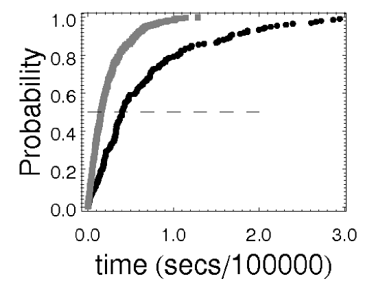
Figure 1: Probability of obtaining target solution value of 21220000 versus time for the Tai100a instance. Lower (black) plot is for RTS only runs; upper (gray) plot is for hybrid heuristic of RTS and VDSS. The intersection of each plot with the dashed line at probability $0.5$ is the time $t_{50}$ used for the performance improvement factor calculation

Figure 1 compares time-to-target plots for RTS runs and hybrid heuristic runs composed of RTS followed by VDSS. A single hybrid heuristic run consists of first running RTS with a random starting configuration and then running VDSS with the RTS solution as input. The instance tested is Tai100a and the target value is 21200000. We will see below that VDSS used alone is inferior to RTS. However, as Figure 1illustrates the hybrid solution of RTS + VDSS provides better performance than RTS alone.

Let the time needed to achieve the target value with $50\%$ probability for a heuristic be $t_{50}$. Then we define the performance improvement factor of the hybrid heuristic (RTS + VDSS) to RTS alone as:

$$I=\frac{t_{50}(RTS)}{t_{50}(RTS+VDSS)}.$$ (7)

The performance improvement factor for Figure 1 is 2.61.

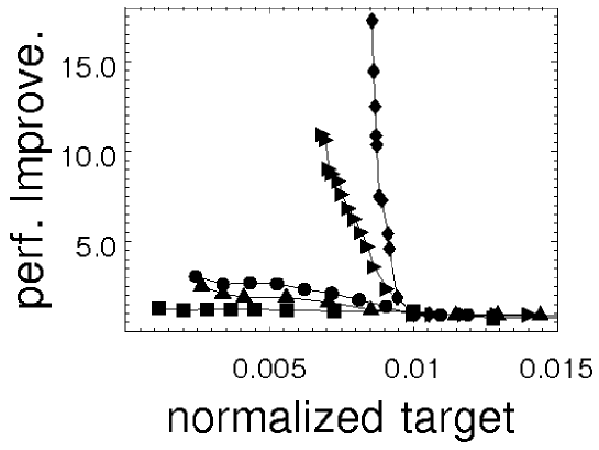
Figure 2: Performance improvement versus normalized target values (see (8) ) for $N=60$ (squares), $80$ (up-triangles), $100$ (disks), $200$ (right-triangles) and $400$ (diamonds). Below the normalized target value of 0.01, the larger the value of $N$ the larger the slopes of the plots.

In Figure. 2 we plot the performance improvement factor for the instances studied versus various target values. Note that for each of the plots, there is a target value above which the plots are essentially flat; the performance improvement is constant and less than $1$ here because RTS alone can reach these targets. Below these improvement thresholds the performance improvement increases with decreasing target values. In order to show the plots in a single figure, we plot performance improvement versus normalized target values

$$\tilde{\tau}=\frac{\tau-b(N)}{b(N)}$$ (8)

where $\tau$ is the non-normalized target value and $b(N)$ is a value which results in the improvement thresholds of the plots being coincident. Having the improvement thresholds coincident makes comparison of the plots easier. We note that

• for a given instance, the performance improvement factor increases as the target value is decreased because, as the target is decreased, RTS alone is less and less likely to reach the target. Running VDSS following RTS, while adding time to a run, makes reaching the target more likely.

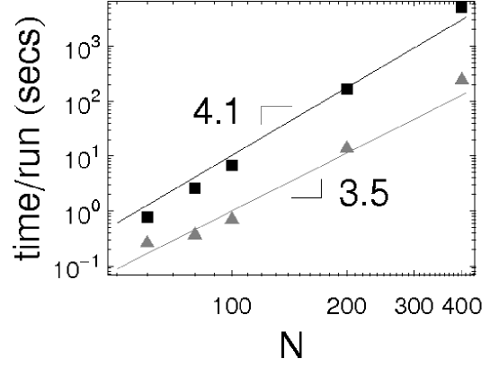
Figure 3: Time per run versus $N$ for RTS (black upper plot) and VDSS (gray lower plot). The slopes on these log-log plots are the power of $N$ of the computational complexity.

• as the instance size increases, the performance improvement increases. Figure 3 plots the time per run as a function of $N$ for RTS, and for VDSS when run following RTS. Note that for RTS the time scales as $N^{x}$ where $x\approx 4.1$. This is consistent with the theoretical estimate that the complexity of RTS is $O(N^{4})$ given that RTS requires $O(N^{2})$ operations per iteration and $N^{2}$ iterations per run. For VDSS the time scales as $N^{y}$ where $y\approx 3.5$. This lower order complexity is one reason the performance improvement of the hybrid algorithm improves as $N$ increases.

In Table 1 we list the instances tested and the results. The lowest target value for which we determine the performance improvement is determined by our ability to perform enough runs which reach that target value to have meaningful statistics. Below the target values shown in Table 1, the time to perform the needed number of runs would have been unreasonably long. Performance improvement results shown in Table 1 are for these lowest target values.

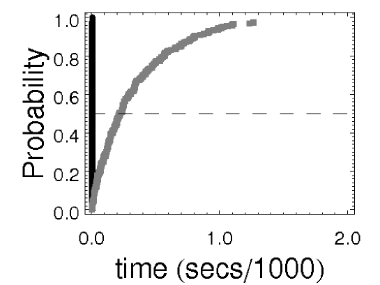
Figure 4: Probability of obtaining target solution value of 21400000 versus time for the Tai100a instance. Black plot is for RTS-only runs; gray plot is for VDSS-only runs. The RTS plot appears essentially straight but would have a similar shape to the VDSS plot if magnified. The intersection of each plot with the dashed line at probability $0.5$ is the time $t_{50}$ used for the performance improvement factor calculation

In Figure 4 we compare the performance of RTS alone and VDSS alone. As opposed to the hybrid heuristic RTS+VDSS, VDSS alone has performance significantly inferior to RTS.

7 Discussion/Conclusions

We use the Lin-Kernighan pruning approach to implement an effective variable depth sequential search which, when used in conjunction with RTS, provides considerable performance improvement over RTS alone. RTS efficiently finds a local minima and VDSS explores the neighborhood around this local minima to improve the solution. Because RTS is a basic building block in a number of hybrid heuristics, the combined RTS+VDSS approach described here may provide further performance improvements for those heuristics which use RTS alone.

To the best of our knowledge this is the first use of the Lin-Kernighan pruning technique for a problem in which the incremental gains for the sequential moves are not independent. Our results raise the question of whether variable depth sequential search with Lin-Kernighan pruning can be applied to other problems in which incremental gains are also not independent and for that reason the Lin-Kernighan approach may have not been applied to them. The code which implements VDSS is available in the Online Supplement and can be used as a model for application to such other problems.

In addition, we introduce two new QAP instances, Pau200a and Pau400a, available in the Online Supplement. As processing speed increases, we expect that there will be a need for instances of this size for QAP heuristics.

Appendix - Moving a node more than once in a sequence

If a node is not allowed to be moved more than once in a sequence, there are certain assignments of nodes to locations which cannot be obtained by a single series of sequential moves starting with a given assignment. For example, the permutation 2,3,1,5,6,4 cannot be transformed into 1,2,3,4,5,6. The transformation can be obtained with two separate series of sequential moves each without moving a node more than once, but if neither of these series of moves results in a positive gain, the pruning algorithm will not allow these moves to be made. If moving a node more than once is allowed, any assignment can be obtained. In practice we have found that there is minimal benefit, if any, to allowing nodes to be moved more than once and have not allowed it in our runs.

References

• Aiex, R.M. 2002. Uma investigacao experimental da distribuicao de probabilidade de tempo de solucao em heuristicas GRASP e sua aplicacao na analise de implementacoes paralelas. PhD thesis, Department of Computer Science, Catholic University of Rio de Janeiro, Rio de Janeiro, Brazil.

• Aiex, R.M., M.G.C. Resende, C.C. Ribeiro. 2002. Probability distribution of solution time in GRASP: An experimental investigation. J. Heuristics 8 343-373.

• Anstreicher, K. 2003. Recent advances in the solution of quadratic assignment problems. Math. Program. 97, 27-42.

• Burkard R.E., E. Cela, S. E. Karish, F. Rendl. 1997. QAPLIB - A Quadratic Assignment Problem Library. J.Global Optim. 10 391-403; http://www.seas.upenn.edu/qaplib/

• Cela E. 1998. The Quadratic Assignment Problem: Theory and Algorithms. Kluwer, Boston, MA.

• Helsgaun K. 2000. An Effective Implementation of the Lin-Kernighan Traveling Salesman Heuristic. Eur. J. Oper. Res. 126 106-130.

• James T., C. Rego, F. Glover. 2009. Multistart Tabu Search and Diversification Strategies for the Quadratic Assignment Problem. IEEE Tran. on Systems, Man, and Cybernetics PART A: SYSTEMS AND HUMANS 39 579-596.

• Koopmans T., M. Beckmann. 1957. Assignment problems and the location of economic activities. Econometrica 25 53-76.

• Lin S., B.W. Kernighan. 1973. An effective heuristic algorithm for the traveling-salesman problem. Operations Research 21 498-516; http://www.cs.bell-labs.com/who/bwk/tsp/index.html.

• Misevicius, A. 2005. A tabu search algorithm for the quadratic assignment problem. Comput. Optim. and Appl. 30 95-111.

• Misevicius, A. 2008 An implementation of the iterated tabu search algorithm for the quadratic assignment problem. Working Paper, Kaunas University of Technology, Kaunas, Lithuania.

• Oliveira, C.A.S., P.M. Pardalos, G. Mauricio, C. Resende. 2004. GRASP with Path-Relinking for the Quadratic Assignment Problem. Ribeiro, C.C. and Martins, S.L. eds., Efficient and Experimental Algorithms, LNCS 3059, 356-368, Springer-Verlag, Berlin.

• Pardalos, P.M., F. Rendl, H. Wolkowicz. 1994. The quadratic assignment problem: A survey and recent developments. Pardalos, P.M., Wolkowicz, H., eds. Quadratic Assignment and Related Problems. DIMACS Series on Discrete Mathematics and Theoretical Computer Science 16, Amer. Math. Soc., Baltimore, MD. 1-42.

• Taillard, E. 1991. Robust taboo search for the quadratic assignment problem. Parallel Comput. 17 443-455..

Table 1: Numerical Results. Improvement threshold is the approximate target value below which the hybrid solution provides a performance improvement $>1$. Target value is the target value for which performance improvement is measured. ^a Misevicius (2005); ^b Misevicius (2008); ^c current work.

Problem	Best known	Improvement	Target	Performance
	solution	threshold	value	improvement
Tai60a	7205962a	7320000	7256000	1.30
Tai80a	13511780b	13720000	13620000	2.52
Tai100a	21052466b	21360000	21200000	3.07
Pau200a	89282330c	89740000	89460000	10.94
Pau400a	366463098c	367600000	367060000	15.15

.

.