Finite dimensional attractor for a composite system of wave/plate equations with localised damping

Francesca Bucci

Università degli Studi di Firenze

Dipartimento di Matematica Applicata

Firenze, 50139, Italy

Daniel Toundykov

University of Nebraska–Lincoln

Department of Mathematics

Lincoln, NE 68588, USA

Abstract. The long-term behaviour of solutions to a model for acoustic-structure interactions is addressed; the system is comprised of coupled semilinear wave (3D) and plate equations with nonlinear damping and critical sources. The questions of interest are: existence of a global attractor for the dynamics generated by this composite system, as well as dimensionality and regularity of the attractor. A distinct and challenging feature of the problem is the geometrically restricted dissipation on the wave component of the system. It is shown that the existence of a global attractor of finite fractal dimension—established in a previous work by Bucci, Chueshov and Lasiecka (Comm. Pure Appl. Anal., 2007) only in the presence of full interior acoustic damping—holds even in the case of localised dissipation. This nontrivial generalization is inspired by and consistent with the recent advances in the study of wave equations with nonlinear localised damping.

1. Introduction

This paper focuses on the long-term behaviour of a system of partial differential equations (PDE’s, or simply PDE) modeling acoustic waves in a three-dimensional domain $\Omega$, and their interaction with the elastic vibrations of a part $\Gamma_{0}\subset\Gamma:=\partial\Omega$ of the boundary. The corresponding PDE problem ((2.1) below) is comprised of semilinear wave and plate equations on domains $\Omega$ and $\Gamma_{0}$ respectively; a detailed description of the system will be given in the next section.

PDE models for acoustic-structure interactions have received a great deal of attention in the past decade, mainly in the context of control theory, in connection with (but not limited to) the problem of reducing the noise inside an acoustic chamber and stabilizing its vibrating walls. As in the case of a single PDE, the sought-after properties—on a theoretical level, yet with implications for the computational methods—are (besides well-posedness): stability, controllability, and solvability of the associated optimal control problems. However, the presence of two (or more) coupled equations, of different type (usually, hyperbolic and parabolic) and/or acting on manifolds of different dimensions, renders the PDE analysis of the dynamics far more complex.
It is beyond this work’s scope to provide a comprehensive account of the literature on control problems for such interconnected PDE systems. However, for completeness and the reader’s convenience some notable contributions are listed below.

Deep insight into the physical origin of PDE models for acoustic-structure interactions is provided by [47]. A more recent reference on analytical methods for modeling acoustic problems is [36].

A general reference for the mathematical control theory of established coupled PDE systems for acoustic-structure interactions is the treatise [40], which also contains an extensive bibliography, from which we explicitly cite [2] (PDE analysis and optimal control), [3, 4] (controllability), and [45, 41] (uniform stability), besides the former [25], [8], [46].

More recent advances include, for instance (without any claim of completeness), [42], [44] and [1] (general theory of quadratic optimal control and of Riccati equations), [9, 10] (sharp interior/boundary regularity, with application to optimal control), [12] (stabilization). For a survey of results on exact boundary controllability and uniform boundary stabilizability by differential geometric methods, see [34]. The stability of an interesting 2D structural-acoustic model was discussed in [32, 33].

The focus of this study is on the long-term behavior of the nonlinear dynamics generated by the system (2.1) below, such as existence of a global attractor and its properties: geometry, fractal dimension, regularity. It was shown in [11] that in the presence of an acoustic dissipation distributed over the entire domain $\Omega$, existence of a global attractor is guaranteed under some basic assumptions on all the nonlinearities, including the most relevant case when the function modeling the acoustic source has a critical exponent. Furthermore, even under a critical, i.e. non-compact, perturbation the attractor has a finite fractal dimension, provided the dissipation terms acting on either equation satisfy suitable conditions; in particular, the acoustic dissipation must be linearly bounded.

In light of the recent advances in the study of the long-term behaviour of wave equations with nonlinear damping [21, 22], the present work aims at showing that dissipation active only in a neighbourhood of $\Gamma_{0}$—combined with a nonlinear interior plate damping, as in the PDE model addressed in [11]—still guarantees the existence of a finite-dimensional global attractor.

With this as background motivation, let us now discuss the major challenges which arise in the present context of

• coupled hyperbolic PDE’s (wave and plate equations),

• localised damping in conjunction with a critical exponent-source on the wave equation,

• a critical-exponent source on the plate equation,

and then describe the principal theoretical and technical arguments utilized to overcome them.

1.1. New challenges

Critical sources alone have been well-known to present an intrinsic obstacle to formation of attractors. At the level of critical-exponents the compactness of corresponding Sobolev embeddings is lost, and “critical terms” are essentially non-compact perturbations of the principal dynamics. Thus, in general, one would not expect the flow to converge to a compact set, especially in hyperbolic systems. For an overview of associated challenges see the very comprehensive treatise [20]. The recent advances in this direction, however, predominantly rely on the dissipation mechanism being supported on the entire domain. In particular, for structural acoustic interactions, it was shown in [11] that in the presence of an acoustic dissipation distributed over the whole domain domain $\Omega$, is sufficient for existence of a global finite-dimensional attractor, even in presence of a critical acoustic source.

However, the physically relevant localised interior (or boundary) damping poses yet further difficulties, since besides the lack of compactness from criticality, the dissipation now must be “propagated” across the domain in order to have any kind of a stabilizing effect. A critical source and geometrically restricted damping in a single wave equation had been a long-standing open problem, whose solution ultimately necessitated Carleman estimates and geometric optics analysis [21, 22].

In a composite setting the aforementioned techniques would have to account not merely for two different types of dynamics, but also for the Neumann-type coupling on the interface. Moreover, the source on the plate is described by higher-order operators and, if approached via the same strategy as the acoustic counterpart, presents a much more formidable obstacle. To overcome this difficulty, we develop a new “hybrid” method that employs different techniques applicable to waves with localised damping, while taking advantage of the full interior dissipation on the plate; at the same time the analysis accommodates the mixed terms that arise from the coupling.

Ultimately it follows that acoustic damping active only in a neighbourhood of the flexible boundary—combined with a nonlinear interior plate damping—still guarantees the existence of a finite-dimensional global attractor, under “minimal” assumptions on the nonlinear functions; “minimal” here indicating those consistent with the hypotheses which yield a global attractor for the dynamics generated by a single wave equation.

1.2. Outline of the argument

To achieve our goal we will appeal to several general criteria from the theory of infinite-dimensional dynamical systems. While well-posedness follows via the classical theory of monotone operators in [6], along with some recent additions devised in [16], the asymptotic analysis will benefit from novel abstract results gathered in [20], specifically tailored for dissipative evolution equations of hyperbolic type. (For general references on dissipative infinite-dimensional systems, the reader is referred to the cornerstones: [5], [53] and [35]; see also [39] and [14], the latter addressing non-autonomous systems.) More specifically, we shall invoke

1. a compactness criterion—introduced in [37] and subsequently recast into a more general abstract form in [19]—recorded here as Theorem A.2 (this result is central to the proof of existence of a global attractor),

2. a generalization of Ladyzhenskaia’s Theorem on dimension of invariant sets, that is Theorem A.4, which will finally enable us to infer finite-dimensionality of the attractor.

The application of the aforesaid criteria is not immediate, as one might guess in light of the analysis already carried out on the composite PDE system in [11] with (acoustic) full interior damping, and of the novel tools devised in [21] for the (uncoupled) wave equation with localised dissipation. A primary source of difficulty stems from the fact that these abstract results require estimates on the quadratic energy corresponding to the difference of two trajectories, rather than to a single trajectory, and the presence of localised acoustic dissipation in conjunction with the coupling (with the plate equation) brings about further technical difficulties, over those encountered in [11] and [21], as explained in §1.1.

The analysis to be carried out includes various steps. After a preliminary discussion of well-posedness of the PDE system in an appropriate state space, a major task will be to establish asymptotic compactness. That the global attractor has a finite fractal dimension will be obtained subsequently, through a use of both a Carleman-like identity established in [21] for the wave dynamics, and exploiting the attractor’s compactness. As expected, proving finite dimensionality and the additional smoothness of the attractor will require stronger assumptions on the nonlinear dissipation terms in either of the coupled equations.

Note that we chose to separate the proof of existence of a global attractor from that of its finite-dimensionality, as the former property does hold under weaker assumptions. In this respect, the present argument differs from the ones followed in a large part of the recent literature on dissipative dynamical systems, where existence of an exponential attractor is sought, as it brings about—besides a certain robustness under perturbations and numerical approximations—the intrinsic feature of finite dimensionality; see, e.g. (and without any claim of completeness), [27], [28], [29], [30], [31], [50]. The question whether the PDE system under investigation possesses an exponential attractor will not be discussed here.

We finally note that the boundedness of the attractor in a smoother functional space is closely tied to its finite-dimensionality. The proofs of both results are interconnected; it is precisely the compactness of the attractor in the finite-energy space and the regularity estimate in the higher-energy space which together show that critical (non-compact) sources, do not substantially perturb the structure of the attracting set. A recent result [24] provides an elegant way to prove regularity of a global attractor in higher norms, without directly appealing to uniform-in-time estimates; however, the application of this argument to a wave equation requires a stronger damping than employed in the present case.

A brief outline of the paper follows.

• In Section 2 we introduce the PDE model under investigation, along with the statements of our main results: well-posedness (Theorem 2.4), existence of a global attractor for the corresponding dynamics (Theorem 2.5), and finite-dimensionality, as well as regularity of the attractor (Theorem 2.7). The natural energies and state spaces for either uncoupled equation, and then for the coupled PDE system, are introduced and briefly discussed in Section 2.2.

• Section 3 contains some preliminary work for the proof of existence of the attractor. More precisely, we establish a basic identity involving the integral of the quadratic wave and plate energies pertaining to the differences of trajectories; see Lemma 3.4.

• Section 4 is devoted to the proof of Theorem 2.5. Existence of a global attractor is established in view of the gradient structure of the dynamical system and asymptotic smoothness of the semi-flow. In turn, this latter (crucial) property follows from a pointwise estimate of the total quadratic energy (Proposition 4.2), combined with a suitable “weak sequential compactness” property (Proposition 4.3).

• Section 5 is focused on the proof of Theorem 2.7, technically based on the key inequality established in Lemma 5.1 (refined in Lemma 5.3), and on the Proposition 5.4. Finally, a short Appendix concludes the paper.

2. The PDE model and the statement of main results

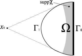
The PDE system under investigation models structure-acoustics interactions described by the acoustic velocity potential $\zeta(x,t)$ evolving in a smooth domain $\Omega\subset\mathbb{R}^{3}$, and the vertical displacement $w(x,t)$ of a thin hinged plate whose midsection occupies a part of the boundary of $\Omega$; we denote the latter by $\Gamma:=\partial\Omega$, and assert that it consists of two relatively open simply-connected segments with overlapping closures $\Gamma_{0}\cup\Gamma_{1}$, where $\Gamma_{0}$ represents the plate, and $\Gamma_{1}$ is the rigid wall of the acoustic chamber. The acoustic damping is confined to a subset of $\Omega$ corresponding to the support of the cutoff function $\chi(x)$.

(2.1) $$\left\{\begin{array}[]{lll}\zeta_{tt}-\Delta\zeta+\chi(x)g(\zeta_{t})=f(\zeta)&{\rm in}&\Omega\times(0,T)\\[5.69054pt] \displaystyle\frac{\partial\zeta}{\partial\nu}=0&{\rm on}&\Gamma_{1}\times(0,T)\\[5.69054pt] \displaystyle\frac{\partial\zeta}{\partial\nu}=\alpha\kappa\,w_{t}&{\rm on}&\Gamma_{0}\times(0,T)\\[5.69054pt] \zeta(0,\cdot)=\zeta_{0}\,,\quad\zeta_{t}(0,\cdot)=\zeta_{1}&{\rm in}&\Omega\\[5.69054pt] w_{tt}+\Delta^{2}w+b(w_{t})+\beta\kappa\zeta_{t}|_{\Gamma_{0}}=f_{2}(w)&{\rm in}&\Gamma_{0}\times(0,T)\\[5.69054pt] w=\Delta w=0&{\rm on}&\partial\Gamma_{0}\times(0,T)\\[5.69054pt] w(\cdot,0)=w_{0}\,,\quad w_{t}(\cdot,0)=w_{1}&{\rm in}&\Gamma_{0}\,.\end{array}\right.$$

The positive constants $\alpha$, $\beta$ and $\kappa$ represent parameters dictated by the physical model in question. Following [11], we shall consider, specifically,

(2.2) $$f_{2}(w)=p_{0}-\Big{[}Q-\int_{\Gamma_{0}}|\nabla w|^{2}\Big{]}\Delta w\,,$$

which is the semilinear term that occurs in Berger’s plate model: the function $p_{0}$, which is related to transversal forces, belongs to $L_{2}(\Gamma_{0})$, while the real constant $Q$ describes in-plane forces applied to the plate; for more on modeling according to the Berger approach, see [15].

Remark 1.

It is important to emphasise that although we consider a plate equation with a nonlinear term $f_{2}$ of the form (2.2), the analysis carried out in the present paper might be extended to more general nonlinear functions, provided they satisfy proper conditions, such as those listed in Assumption 4.11 in [20] (following this reference’s notation, in the present case ${\mathcal{A}}$ would denote the plate dynamics operator, that is the realization of the bilaplacian $\Delta^{2}$ with hinged boundary conditions).

2.1. Assumptions and main results

Due to geometric restrictions on the acoustic damping, the shape of $\Omega$ must satisfy certain restrictions in order for the feedback $\chi(x)g(\zeta_{t})$ to be “effective,” as dictated by geometric optics and the classical results on propagation of singularities [7]. A sufficient assumption is the following:

Assumption 2.1 (Geometry of the domain).

$\Gamma_{1}$ is a level-surface of a convex function and there exists $x_{0}\in\mathbb{R}^{n}$ such that

$$(x-x_{0})\cdot\nu\leq 0\quad\textrm{on }\;\Gamma_{1}\,,$$

with $\nu$ being the outward normal vector field on $\Gamma_{1}$.

Figure 1 shows what a cross-section of a possible domain may look like.

Figure 1. A cross-section of a suitable domain $\Omega$. The rigid wall $\Gamma_{1}$, and, in particular, the part of the boundary outside $\mbox{supp}\chi$ is convex; however, more general configurations are possible: for other examples see [43].

Remark 2 (More general geometric conditions).

The convexity of $\Gamma_{1}$ is a sufficient requirement, but it is possible to further relax this assumption. In particular, it suffices to ask for the subset of $\Gamma_{1}$ that lies away from $\operatorname{supp}\chi(x)$ to be a level-surface of a function with a non-vanishing gradient and positive-definite or negative-definite Hessian (in the latter case the condition on $x_{0}$ should be changed to $(x-x_{0})\cdot\nu\geq 0$). See [43] for more details and examples.

Assumption 2.2 (Nonlinear terms).

The function $f$ satisfies:

• $f\in C^{2}(\mathbb{R})$ and there exists $C_{f}$ such that

  (2.3) $$|f^{\prime\prime}(s)|\leq C_{f}(1+|s|)\qquad\forall s\in\mathbb{R};$$

• $\displaystyle\limsup_{|s|\to\infty}\frac{f(s)}{s}=:-2\lambda<0$.

Accordingly, set $f_{1}(s)=f(s)+\lambda s$.

Existence of a global attractor will be established under rather weak assumptions on the feedback maps $g$ and $b$.

Assumption 2.3 (Damping terms, I).

1. $g\in C(\mathbb{R})$ is a monotone increasing function such that $g(0)=0$; in addition, $g$ is linearly bounded at infinity, i.e. there exist positive constants $m_{g}$, $M_{g}$ such that

   (2.4) $$m_{g}|s|\leq|g(s)|\leq M_{g}|s|\qquad\textrm{for \;}|s|\geq 1\,.$$

2. $b\in C(\mathbb{R})$ is a monotone increasing function such that $b(0)=0$; and there exists $m_{b}$ such that

   (2.5) $$|b(s)|\geq m_{b}|s|\qquad\textrm{for \;}|s|\geq 1\,.$$

A few comments about the above assumptions are in order. As observed already in [11] and [21], a prime consequence of Assumption 2.2 is local Lipschitz continuity of the nonlinear term $f$ (and of $f_{1}$, as well), as an operator from $H^{1}(\Omega)$ into $L_{2}(\Omega)$. Namely, one has

$$\|f(\zeta_{1})-f(\zeta_{2})\|\leq C(r)\|\zeta_{1}-\zeta_{2}\|_{1,\Omega}\qquad\forall\zeta_{i}\quad\textrm{with}\;\|\zeta_{i}\|_{1,\Omega}\leq r\,,\,i=1,2\,.$$

The above property is easily shown by using well known Sobolev embedding results in $3$-D domains, which establish the critical threshold in the polynomial bound on $f$. The same (Lipschitz continuity) is true for the nonlinear term $f_{2}$ which occurrs in the plate equation; more precisely,

$$\|f_{2}(w_{1})-f_{2}(w_{2})\|\leq C(r)\|w_{1}-w_{2}\|_{2,\Gamma_{0}}\qquad\forall w_{i}\quad\textrm{with}\;\|w_{i}\|_{2,\Gamma_{0}}\leq r\,,\,i=1,2\,.$$

Next, observe that the basic Assumption 2.3 forces the acoustic damping to be linearly bounded at infinity. It is important to emphasise that this condition is actually necessary, because of the geometrical restrictions on the damping term. This fact was first exhibited in [55] for a wave equation with boundary dissipation; indeed, the case of localised dissipation around a portion of the boundary yields the same technical difficulties and the same results as that of boundary damping. The reader is referred to [21, Section 1] for a more detailed discussion of these issues.

The aforementioned basic assumptions are sufficient to establish bothwell-posedness for the PDE problem (2.1) and existence of a global attractor for the corresponding dynamical system.

Theorem 2.4 (Well-posedness).

Define the state space

$${\mathcal{Y}}:=H^{1}(\Omega)\times L^{2}(\Omega)\times H^{2}_{0}(\Gamma_{0})\times L^{2}(\Gamma_{0})\,.$$

The system (2.1) generates a strongly continuous semigroup $S(t)$ on ${\mathcal{Y}}$. In particular, given initial data, at $t=0$, $W_{0}=\{\zeta_{0},\zeta_{1},w_{0},w_{1}\}\in{\mathcal{Y}}$ there exists a unique solution to (2.1)

$$S(\cdot)W=\{\zeta,\zeta_{t},w,w_{t}\}\in C([0,T],{\mathcal{Y}})$$

for any $T\geq 0$. The solution satisfies the following variational identities

(2.6) $$\begin{split}(\zeta_{t},\phi)\bigg{|}_{0}^{T}-\int_{0}^{T}(\zeta_{t},\phi_{t})+\int_{0}^{T}(\nabla\zeta,\nabla\phi)+&\int_{0}^{T}(\chi g(\zeta_{t}),\phi)\\ =&\int_{0}^{T}(f(\zeta),\phi)+\int_{0}^{T}\langle\alpha\kappa w_{t},\phi\rangle\,,\end{split}$$

(2.7) $$\begin{split}\langle w_{t},\psi\rangle\bigg{|}_{0}^{T}-\int_{0}^{T}\langle w_{t},\psi_{t}\rangle+\int_{0}^{T}\langle\Delta w,\Delta\psi\rangle+&\int_{0}^{T}\langle b(w_{t}),\psi\rangle\\ =&\int_{0}^{T}\langle f_{2}(w),\psi\rangle-\int_{0}^{T}\langle\psi,\beta\kappa\zeta_{t}\rangle\,,\end{split}$$

for any test functions

$$\phi\in C^{1}([0,T],L^{2}(\Omega))\cap C([0,T];H^{1}(\Omega))\,,\;\psi\in C^{1}([0,T],L^{2}(\Gamma_{0}))\cap C([0,T];H^{2}_{0}(\Gamma_{0}))\,.$$

Moreover, if the initial data belong to the spaces

$$\{\zeta_{0},\zeta_{1}\}\in H^{2}(\Omega)\times H^{1}(\Omega),\quad\{w_{0},w_{1}\}\in\big{(}H^{4}(\Gamma_{0})\cap H_{2}(\Gamma_{0})\big{)}\times H^{2}_{0}(\Gamma_{0})$$

with the compatibility conditions

$$\frac{\partial\zeta_{0}}{\partial\nu}\Big{|}_{\Gamma_{1}}=0,\qquad\frac{\partial\zeta_{0}}{\partial\nu}\Big{|}_{\Gamma_{0}}=\alpha\kappa w_{1}\,,$$

then

$$\{\zeta,\zeta_{t},w,w_{t}\}\in L^{\infty}\big{(}0,T;H^{2}(\Omega)\times H^{1}(\Omega)\times H^{4}(\Gamma_{0})\times H^{2}(\Gamma_{0})\big{)}\,.$$

We introduce the set ${\mathcal{N}}$ of equilibria for the dynamical system $({\mathcal{Y}},S(t))$; namely

(2.8) $${\mathcal{N}}:=\{W\in\mathcal{Y}\;:\;S(t)W=W\quad\text{for all}\quad t\geq 0\}\,.$$

Theorem 2.5 (Existence of the global attractor).

Suppose that the Assumptions 2.1–2.2 hold. If the damping functions satisfy the Assumption 2.3, then the dynamical system $({\mathcal{Y}},S(t))$ generated by the PDE problem (2.1) has a compact global attractor $\mathscr{A}\subset{\mathcal{Y}}$, which coincides with the unstable manifold $M^{u}({\mathcal{N}})$ of the set ${\mathcal{N}}$ of stationary points:

• $\mathscr{A}\equiv M^{u}({\mathcal{N}})$;

• $\displaystyle\lim_{t\to+\infty}{\rm dist}(S(t)W,{\mathcal{N}})=0\quad\textrm{for any}\quad W\in{\mathcal{Y}}$.

To prove that the attractor has a finite fractal dimension we will need to strengthen the regularity and growth condition on both damping functions.

Assumption 2.6 (Dampings, II).

Assume $g,b\in C^{1}(\mathbb{R})$, with $g(0)=0=b(0)$, and

1. there exist positive constants $m_{g}^{\prime}$, $M_{g}^{\prime}$ such that

   (2.9) $$m_{g}^{\prime}\leq|g^{\prime}(s)|\leq M_{g}^{\prime}\qquad\forall s\in\mathbb{R}\,,$$

2. there exist positive constants $m_{b}^{\prime}$, $M_{b}^{\prime}$ such that

   (2.10) $$m_{b}^{\prime}\leq|b^{\prime}(s)|\leq M_{b}^{\prime}(1+sb(s))\qquad\forall s\in\mathbb{R}\,.$$

Then, the following result holds.

Theorem 2.7 (Finite dimensionality and regularity of the attractor).

Suppose the hypotheses of Theorem 2.5 are satisfied. If, in addition, the Assumption 2.6 holds, then the global attractor $\mathscr{A}$ has a finite fractal dimension.

Furthermore, the attractor $\mathscr{A}$ is bounded in the domain of the nonlinear semigroup generator; in particular, $\mathscr{A}$ is a bounded subset of

$$H^{2}(\Omega)\times H^{1}(\Omega)\times H^{4}(\Gamma_{0})\times H^{2}(\Gamma_{0})\,.$$

2.2. Energy identity and bounds

With the system (2.1) we associate the following energy functionals:

$${\mathcal{E}}_{\zeta}(t) := \frac{1}{2}\left(\|\nabla\zeta\|^{2}+\lambda\|\zeta\|^{2}+\|\zeta_{t}\|^{2}\right)-\int_{\Omega}F_{1}(\zeta(t))$$

$${\mathcal{E}}_{w}(t) := \frac{1}{2}\Big{(}\|\Delta w\|^{2}+\frac{1}{2}\|\nabla w\|^{4}+\|w_{t}\|^{2}\Big{)}-\Pi(w(t))\,,$$

where $F_{1}(s)$ is the antiderivative of $f_{1}(s)$ vanishing at $0$, and

(2.11) $$\Pi(w)=(p_{0},w)+\frac{Q}{2}\|\nabla w\|^{2}-\frac{1}{4}\|\nabla w\|^{4}\,.$$

Define the total energy

(2.12) $${\mathcal{E}}(t)={\mathcal{E}}_{\zeta,w}(t):=\beta{\mathcal{E}}_{\zeta}(t)+\alpha{\mathcal{E}}_{w}(t)\,.$$

The following identity satisfied by ${\mathcal{E}}(t)$ is standard due to the fact that the dissipation feedbacks are linearly bounded at infinity and the sources correspond to locally Lipschitz operators on the energy space. The equation can be derived for strong solutions by using test functions $\beta\zeta_{t}$ and $\alpha w_{t}$ in the variational identities (2.6) and (2.7) respectively. Since the result is continuous with respect to the finite-energy topology, it can be extended to all weak solutions:

(2.13) $${\mathcal{E}}(t)+\beta\int_{s}^{t}(\chi g(\zeta_{t}),\zeta_{t})+\alpha\int_{s}^{t}(b(w_{t}),w_{t})={\mathcal{E}}(s)\,.$$

Also, let us introduce positive quadratic energy functionals:

$$E_{\zeta}(t):=\frac{1}{2}\big{(}\|\nabla\zeta\|^{2}+\lambda\|\zeta\|^{2}+\|\zeta_{t}\|^{2}\big{)}\,,\quad E_{w}(t):=\frac{1}{2}\Big{(}\|\Delta w\|^{2}+\frac{1}{2}\|\nabla w\|^{4}+\|w_{t}\|^{2}\Big{)}\,;$$

(2.14) $$E(t)=E_{\zeta,w}(t):=E_{\zeta}(t)+E_{w}(t)\,.$$

Owing to the dissipativity property (in Assumption 2.2) satisfied by $f$ and to the structure of the functional $\Pi$ in (2.11), it is not difficult to obtain upper and lower bounds for the full energy of the system; see also [11, Section 2.2]. Explicit computations pertaining to the wave component are found in [16, Section 2].

Proposition 2.8 (Bounds on the energy).

Let ${\mathcal{B}}$ be a bounded subset of ${\mathcal{Y}}$. If $\{\zeta_{0},\zeta_{1},w_{0},w_{1}\}\in{\mathcal{B}}$ then there exists constants $C_{1,{\mathcal{B}}},C_{2,{\mathcal{B}}}$ dependent only on the diameter of ${\mathcal{B}}$ (in the topology of ${\mathcal{Y}}$) such that

(2.15) $$C_{1,{\mathcal{B}}}E(t)-C_{2,{\mathcal{B}}}\leq{\mathcal{E}}(t)\leq{\mathcal{E}}(0)\qquad\forall t\geq 0\,.$$

We conclude this section by introducing the abstract dynamic operators pertaining to either equation, namely:

$$A_{1}v=-\Delta v,\quad{\mathcal{D}}(A_{1})=\Big{\{}v\in H^{2}(\Omega)\,:\;\frac{\partial v}{\partial\nu}\Big{|}_{\Gamma}=0\Big{\}}\,;$$

$$A_{2}v=\Delta^{2}v,\quad{\mathcal{D}}(A_{2})=\Big{\{}v\in H^{4}(\Gamma_{0})\cap H^{1}_{0}(\Gamma_{0})\,:;\Delta v\big{|}_{\partial\Gamma_{0}}=0\Big{\}}\,.$$

3. The differences of trajectories: introductory results

Seeking to apply the abstract results recorded in the Appendix as Theorem A.2 and Theorem A.4, to investigate the asymptotic behaviour of the solutions to (2.1), we must study differences of its trajectories, rather than the trajectories themselves. In this section we introduce the relative basic definitions, along with a series of preliminary identities which constitute a first step in the proof of our main results.

3.1. Auxiliary functions and parameters

Given two different evolution trajectories $(h,h_{t},u,u_{t})$ and $(\zeta,\zeta_{t},w,w_{t})$ of the coupled PDE system (2.1), we introduce the differences $z$ and $v$, namely,

(3.1) $$z :=h-\zeta\,,\qquad(\zeta=h+z\,);$$

(3.2) $$v :=u-w\,,\qquad(u=w+v\,).$$

The pair $(z,v)$ readily solves the new coupled system

(3.3) $$\left\{\begin{array}[]{lll}z_{tt}-\Delta z+\lambda z+\chi(x){\tilde{g}}(\zeta_{t})={\tilde{f_{1}}}(z)&{\rm in}&\Omega\times(0,T)\\[5.69054pt] \displaystyle\frac{\partial z}{\partial\nu}=0&{\rm on}&\Gamma_{1}\times(0,T)\\[5.69054pt] \displaystyle\frac{\partial z}{\partial\nu}=\alpha\kappa\,v_{t}&{\rm on}&\Gamma_{0}\times(0,T)\\[5.69054pt] z(0,\cdot)=h_{0}-\zeta_{0}\,,\quad z_{t}(0,\cdot)=h_{1}-\zeta_{1}&{\rm in}&\Omega\\[5.69054pt] v_{tt}+\Delta^{2}v+{\tilde{b}}(w_{t})+\beta\kappa z_{t}|_{\Gamma_{0}}={\tilde{f_{2}}}(v)&{\rm in}&\Gamma_{0}\times(0,T)\\[5.69054pt] v=\Delta v=0&{\rm on}&\partial\Gamma_{0}\times(0,T)\\[5.69054pt] v(0,\cdot)=u_{0}-w_{0}\,,\quad v_{t}(0,\cdot)=u_{1}-w_{1}&{\rm in}&\Gamma_{0}\,.\end{array}\right.$$

where we have set

(3.4) $${\tilde{g}}(z_{t}) :=g(\zeta_{t}+z_{t})-g(\zeta_{t})\,,$$

(3.5) $${\tilde{b}}(v_{t}) :=b(w_{t}+v_{t})-b(w_{t})\,,$$

(3.6) $${\tilde{f_{1}}}(z) :=f_{1}(\zeta+z)-f_{1}(\zeta)\,,$$

(3.7) $${\tilde{f_{2}}}(v) :=f_{2}(w+v)-f_{2}(w)\,.$$

Technically each of the introduced functions also depends on one of the terms in the corresponding difference, but that fact will be suppressed for brevity of notation.

3.2. Smooth cutoff functions

Following [54, Section 6], we introduce two smooth cutoff functions whose role is to single out in $\Omega$ the dissipative and the non-dissipative subdomains. More precisely, $\psi,\phi:\overline{\Omega}\to[0,1]$ are $C^{2}$ functions with the following properties:

• ${\rm supp}(\phi)\subset{\rm supp}(\chi)$,

• $\Omega\setminus{\rm supp}(\chi)\subset\{x:\,\psi(x)=1\}$,

• $\psi\equiv 0$ in a neighbourhood of $\Gamma_{0}$,

• for any $x\in\overline{\Omega}$ at least one of $\psi(x)$ and $\phi(x)$ equals $1$, namely

  $$\{x\in\overline{\Omega}:\psi(x)<1\}\subset\phi^{-1}(\{1\})\,.$$

By setting ${\hat{z}}:=\psi z$ and ${\overset{\scriptscriptstyle\circ}{z}}:=\phi z$, it is easily verified that ${\hat{z}}$ and ${\overset{\scriptscriptstyle\circ}{z}}$ satisfy

(3.8) $${\hat{z}}_{tt}-\Delta{\hat{z}}+\lambda{\hat{z}}+[\![\Delta,M_{\psi}]\!]z+\psi\chi{\tilde{g}}(z_{t})=\psi{\tilde{f_{1}}}(z)\,,$$

(3.9) $${\overset{\scriptscriptstyle\circ}{z}}_{tt}-\Delta{\overset{\scriptscriptstyle\circ}{z}}+\lambda{\overset{\scriptscriptstyle\circ}{z}}+[\![\Delta,M_{\phi}]\!]z+\phi\chi{\tilde{g}}(z_{t})=\phi{\tilde{f_{1}}}(z)\,,$$

where $M_{\psi}$, $M_{\phi}$ denote pointwise (a.e.) multiplication by $\psi$ or $\phi$, respectively, while the pairing $[\![\cdot,\cdot]\!]$ denotes a commutator, acting as follows:

$$[\![\Delta,M_{\psi}]\!]z:=\Delta(\psi z)-\psi\Delta z\,.$$

A straightforward computation gives the equivalent form

(3.10) $$[\![\Delta,M_{\psi}]\!]z=\Delta\psi\,z+2\nabla\psi\nabla z\,.$$

3.3. Vector field ${\mathbf{h}}$

Let us recall from [21] the construction of a function $d$ and the vector field

(3.11) $${\mathbf{h}}(x):=\nabla d(x)\,,$$

whose key properties are

1. (3.12) $$\min_{x\in\overline{\Omega}}d(x)>0\,;$$

2. (3.13) $$({\mathbf{h}}\cdot\nu)|_{\Gamma_{1}}=\frac{\partial d}{\partial\nu}\Big{|}_{\Gamma_{1}}\equiv 0\,;$$

3. the Jacobian matrix $J_{{\mathbf{h}}}$ of ${\mathbf{h}}$—which coincides with the hessian matrix $H_{d}$ of $d$—evaluated on $\Gamma_{1}$ is positive definite. In particular, $d$ can be extended to some open set containing all of $\bar{\Omega}$ so that for some $\rho>0$ one has

   (3.14) $$H_{d}=J_{{\mathbf{h}}}\geq\rho\,I\quad\forall x\in\Omega\,.$$

   The reader is referred to [43, p. 301-303] for more details.

The (Carleman-type) estimates pertaining to the wave component of the system will involve the pseudo-convex function $\Phi:\Omega\times\mathbb{R}\to\mathbb{R}$ defined by

(3.15) $$\Phi(x,t):=d(x)-c\big{|}t-T/2\big{|}^{2}\,,$$

where at the outset $T>0$ and $c$ is a non-negative constant, with $T$ large enough to satisfy

(3.16) $$T>2\big{(}\displaystyle\max_{x\in\overline{\Omega}}d(x)/c\big{)}^{1/2}\,,$$

thus ensuring $\Phi(x,0),\Phi(x,T)<0$.

3.4. Preliminary fundamental identities

3.4.1. Wave component

Our starting point is a key identity pertaining to the wave component of the PDE system (3.3) satisfied by the differences $(z,v)$. This result has been established in [21]; see Proposition 5 in §6.4 therein. Because of the slightly different wave energy, in the present case the identity reads as follows.

Proposition 3.1 (Wave Fundamental identity (Carleman-type), [21]).

Suppose that the Assumptions 2.1, 2.2, 2.3 hold. Take smooth initial data $(\zeta_{0},\zeta_{1}),(h_{0},h_{1})\in{\mathcal{D}}(A_{1})$, and set $z=h-\zeta$. Let $\Phi(x,t)$ be given by (3.15), and let ${\mathbf{h}}:=\nabla\Phi=\nabla d$. Recall the notation ${\hat{z}}:=\psi z$ and ${\overset{\scriptscriptstyle\circ}{z}}:=\phi z$ ($\psi$, $\phi$ are the cutoff functions introduced in Section 3.2). Then, for any $\tau\geq 0$ and any positive constant ${\boldsymbol{\mathcal{C}}}$ one has

(3.17) $$\boxed{\begin{split}\int_{Q_{T}}e^{\tau\Phi}&(J_{{\mathbf{h}}}-\rho Id)\nabla{\hat{z}}\cdot\nabla{\hat{z}}+[Energy]_{\psi}+{\boldsymbol{\mathcal{C}}}\,[Energy]_{\phi}\\ &=[Damping]-\tau\int_{Q_{T}}e^{-\tau\Phi}{\mathcal{M}}_{1}^{2}+\int_{Q_{T}}\psi\big{(}{\tilde{f_{1}}}(z)-\chi{\tilde{g}}(z_{t})\big{)}{\mathcal{M}}_{1}\\ &\quad-\int_{Q_{T}}([\![\Delta,M_{\psi}]\!]z)\,{\mathcal{M}}_{1}+[\text{Almost lower order}]\\ &\quad+\,(BT)_{\Sigma}-\widehat{C}_{0,T}-{\boldsymbol{\mathcal{C}}}\,\overset{\circ}{C}_{0,T}\,,\end{split}}$$

with ${\mathcal{M}}_{1}$ and $\mu$ defined by

(3.18a) $${\mathcal{M}}_{1}:=e^{\tau\Phi}\big{(}{\mathbf{h}}\cdot\nabla{\hat{z}}-\Phi_{t}{\hat{z}}_{t}\big{)}\,,$$

(3.18b) $$\mu:={\rm div}\,(e^{\tau\Phi}{\mathbf{h}})-\partial_{t}(e^{\tau\Phi}\Phi_{t})\,,$$

and

(3.19) $$[Energy]_{\psi}:=\left(\frac{\rho}{2}-c\right)\int_{Q_{T}}e^{\tau\Phi}\big{(}|\nabla{\hat{z}}|^{2}+\lambda{\hat{z}}^{2}+{{\hat{z}}}_{t}^{2}\big{)}\,,$$

(3.20) $$[Energy]_{\phi}:=\int_{Q_{T}}e^{\tau\Phi}\left(|\nabla{\overset{\scriptscriptstyle\circ}{z}}|^{2}+\lambda{\overset{\scriptscriptstyle\circ}{z}}^{2}+{{\overset{\scriptscriptstyle\circ}{z}}}_{t}^{2}\right)\,;$$

moreover, we set

(3.21) $$\begin{split}[Damping]:=\,&2\,{\boldsymbol{\mathcal{C}}}\int_{Q_{T}}e^{\tau\Phi}{\overset{\scriptscriptstyle\circ}{z}}_{t}^{2}-\int_{Q_{T}}\psi\chi{\tilde{g}}(z_{t}){\hat{z}}\left[\frac{\mu}{2}-\big{(}\frac{\rho}{2}+c\big{)}e^{\tau\Phi}\right]\\ &\quad-\,{\boldsymbol{\mathcal{C}}}\int_{Q_{T}}\phi\chi{\tilde{g}}(z_{t})e^{\tau\Phi}{\overset{\scriptscriptstyle\circ}{z}}\,,\end{split}$$

and

(3.22) $$[\text{Almost lower order}]:=-\int_{Q_{T}}{\hat{z}}\nabla{\hat{z}}\cdot\nabla\Big{(}\frac{\mu}{2}-\big{(}\frac{\rho}{2}+c\big{)}e^{\tau\Phi}\Big{)}$$

$$+\int_{Q_{T}}{\hat{z}}{\hat{z}}_{t}\frac{\partial}{\partial t}\Big{(}\frac{\mu}{2}-\big{(}\frac{\rho}{2}+c\big{)}e^{\tau\Phi}\Big{)}+{\boldsymbol{\mathcal{C}}}\int_{Q_{T}}{\overset{\scriptscriptstyle\circ}{z}}{\overset{\scriptscriptstyle\circ}{z}}_{t}\frac{\partial}{\partial t}e^{\tau\Phi}-{\boldsymbol{\mathcal{C}}}\int_{Q_{T}}{\overset{\scriptscriptstyle\circ}{z}}\nabla{\overset{\scriptscriptstyle\circ}{z}}\cdot\nabla e^{\tau\Phi}$$

$$-\int_{Q_{T}}\Big{(}[\![\Delta,M_{\psi}]\!]z-\psi{\tilde{f_{1}}}(z)\Big{)}\Big{\{}{\mathcal{M}}_{1}+{\hat{z}}\Big{[}\frac{\mu}{2}-\big{(}\frac{\rho}{2}+c\big{)}e^{\tau\Phi}\Big{]}\Big{\}}$$

$$-\lambda\int_{Q_{T}}{\hat{z}}\Big{[}{\mathcal{M}}_{1}+{\hat{z}}\big{(}\frac{\mu}{2}+\rho e^{\tau\Phi}\big{)}\Big{]}$$

$$-{\boldsymbol{\mathcal{C}}}\int_{Q_{T}}\big{(}\,[\![\Delta,M_{\phi}]\!]z-\phi{\tilde{f_{1}}}(z)\,\big{)}e^{\tau\Phi}{\overset{\scriptscriptstyle\circ}{z}}\,.$$

The boundary terms are collected in $(BT)_{\Sigma_{T}}$:

(3.23) $$\begin{split}(BT)_{\Sigma_{T}}:=\,&\int_{\Sigma_{T}}\frac{\partial{\hat{z}}}{\partial\nu}{\mathcal{M}}_{1}+\int_{\Sigma_{T}}\frac{\partial{\hat{z}}}{\partial\nu}{\hat{z}}\left[\frac{\mu}{2}-\big{(}\frac{\rho}{2}+c\big{)}e^{\tau\Phi}\right]\\ &+\,\frac{1}{2}\,\int_{\Sigma_{T}}e^{\tau\Phi}\big{(}{\hat{z}}_{t}^{2}-|\nabla{\hat{z}}|^{2}\big{)}({\mathbf{h}}\cdot\nu)\,.+{\boldsymbol{\mathcal{C}}}\int_{\Sigma_{T}}\frac{\partial{\overset{\scriptscriptstyle\circ}{z}}}{\partial\nu}{\overset{\scriptscriptstyle\circ}{z}}e^{\tau\Phi}\,;\end{split}$$

while $\widehat{C}_{0,T}$ and $\overset{\circ}{C}_{0,T}$ are given, respectively, by:

$$\widehat{C}_{0,T} :=\Big{[}\int_{\Omega}e^{\tau\Phi}{\hat{z}}_{t}({\mathbf{h}}\cdot\nabla{\hat{z}})\Big{]}_{0}^{T}-\frac{1}{2}\Big{[}\int_{\Omega}e^{\tau\Phi}\Phi_{t}({\hat{z}}_{t}^{2}+|\nabla{\hat{z}}|^{2})\Big{]}_{0}^{T}$$

(3.24a) $$\qquad\qquad+\,\Big{[}\int_{\Omega}{\hat{z}}_{t}{\hat{z}}\Big{(}\frac{\mu}{2}-\big{(}\frac{\rho}{2}+c\big{)}e^{\tau\Phi}\Big{)}\Big{]}_{0}^{T}\,,$$

(3.24b) $$\overset{\circ}{C}_{0,T} :=\Big{[}\int_{\Omega}{\overset{\scriptscriptstyle\circ}{z}}_{t}{\overset{\scriptscriptstyle\circ}{z}}e^{\tau\Phi}\Big{]}_{0}^{T}\,.$$

Remark 3.

The proof of Proposition 3.1 is rather technical; it involves successive application of weighted multipliers: ${\mathcal{M}}_{1}$, ${\mathcal{M}}_{2}=\mu{\hat{z}}$ (${\mathcal{M}}_{1}$ and $\mu$ are defined in (3.18)) and ${\mathcal{M}}_{3}=e^{-\tau\Phi}{\overset{\scriptscriptstyle\circ}{z}}$. The reader is referred to [21, Section 7.3] for all the details.

Rewriting the fundamental identity (3.17) for $c,\tau=0$ or, equivalently, substituting the identity $I$ in place of $e^{\tau\Phi}$ and utilizing the ‘simplified’ multipliers

$${\mathcal{M}}_{1}={\mathbf{h}}\cdot\nabla{\hat{z}}\,,\qquad\mu={\rm div}\,{\mathbf{h}}\,,$$

we obtain the following basic assertion, which is Proposition 3 in [21, §5.1].

Lemma 3.2 (Wave Basic Identity).

Suppose that the Assumptions 2.1, 2.2, 2.3 hold. Take smooth initial data $(\zeta_{0},\zeta_{1}),(h_{0},h_{1})\in{\mathcal{D}}(A_{1})$, and set $z=h-\zeta$. Recall the notation ${\hat{z}}:=\psi z$ and ${\overset{\scriptscriptstyle\circ}{z}}:=\phi z$ ($\psi$, $\phi$ are the cutoff functions introduce in Section 3.2), and the vector field ${\mathbf{h}}$. Then, for any positive constant ${\boldsymbol{\mathcal{C}}}$ one has

(3.25) $$\begin{split}\int_{Q_{T}}(J_{{\mathbf{h}}}-\rho I)&\nabla{\hat{z}}\cdot\nabla{\hat{z}}+\frac{\rho}{2}\,\int_{Q_{T}}\big{(}|\nabla{\hat{z}}|^{2}+\lambda{\hat{z}}^{2}+{{\hat{z}}}_{t}^{2}\big{)}+{\boldsymbol{\mathcal{C}}}\,\int_{Q_{T}}\big{(}|\nabla{\overset{\scriptscriptstyle\circ}{z}}|^{2}+\lambda{\overset{\scriptscriptstyle\circ}{z}}^{2}+{{\overset{\scriptscriptstyle\circ}{z}}}_{t}^{2}\big{)}\\ &=2\,{\boldsymbol{\mathcal{C}}}\int_{Q_{T}}{\overset{\scriptscriptstyle\circ}{z}}_{t}^{2}+\lambda\rho\int_{Q_{T}}{\hat{z}}^{2}-\frac{1}{2}\int_{Q_{T}}{\hat{z}}\nabla{\hat{z}}\cdot\nabla{\rm div}{\mathbf{h}}\\ &\quad-\int_{Q_{T}}\Big{(}\psi\chi{\tilde{g}}(z_{t})+[\![\Delta,M_{\psi}]\!]z-\psi{\tilde{f_{1}}}(z)\Big{)}\big{[}{\mathbf{h}}\cdot\nabla{\hat{z}}+\frac{{\hat{z}}}{2}({\rm div}{\mathbf{h}}-\rho)\big{]}\\ &\quad-{\boldsymbol{\mathcal{C}}}\int_{Q_{T}}\Big{(}\phi\chi{\tilde{g}}(z_{t})+[\![\Delta,M_{\phi}]\!]z-\phi{\tilde{f_{1}}}(z)\Big{)}{\overset{\scriptscriptstyle\circ}{z}}\\ &\quad+\,(BT)_{\Sigma}-{C}_{0,T}^{w}\,,\end{split}$$

where

(3.26) $$\begin{split}(BT)_{\Sigma}:=&\int_{\Sigma}({\mathbf{h}}\cdot\nabla{\hat{z}})\,\frac{\partial{\hat{z}}}{\partial\nu}+\frac{1}{2}\int_{\Sigma}{\hat{z}}\frac{\partial{\hat{z}}}{\partial\nu}({\rm div}{\mathbf{h}}-\rho)\\ &\qquad+\frac{1}{2}\int_{\Sigma}\big{(}{\hat{z}}_{t}^{2}-|\nabla{\hat{z}}|^{2}-\lambda{\hat{z}}^{2}\big{)}({\mathbf{h}}\cdot\nu)+{\boldsymbol{\mathcal{C}}}\int_{\Sigma}{\overset{\scriptscriptstyle\circ}{z}}\frac{\partial{\overset{\scriptscriptstyle\circ}{z}}}{\partial\nu}\,,\end{split}$$

and

(3.27) $$C_{0,T}^{w}:=\Big{[}\int_{\Omega}{\hat{z}}_{t}\,{\mathbf{h}}\cdot\nabla{\hat{z}}\Big{]}_{0}^{T}+\frac{1}{2}\,\Big{[}\int_{\Omega}{\hat{z}}{\hat{z}}_{t}\,({\rm div}{\mathbf{h}}-\rho)\Big{]}_{0}^{T}+{\boldsymbol{\mathcal{C}}}\Big{[}\int_{\Omega}{\overset{\scriptscriptstyle\circ}{z}}_{t}{\overset{\scriptscriptstyle\circ}{z}}\Big{]}_{0}^{T}\,.$$

3.4.2. Plate component

Let us now turn to the plate equation. The abstract equation satisfied by the difference of two evolution trajectories reads as follows:

(3.28) $$v_{tt}+A_{2}v+{\tilde{b}}(v_{t})+\beta\kappa N_{0}^{*}Az_{t}={\tilde{f_{2}}}(v)\,,$$

where ${\tilde{b}}$ and ${\tilde{f_{2}}}$ are defined in (3.5) and (3.7), respectively, and

$$N_{0}:H^{s}(\Gamma_{0})\to H^{s+3/2}(\Omega)$$

is the extension operator

$$N_{0}\,g=w\quad\Longleftrightarrow\quad\begin{cases}(\lambda I-\Delta)w=0&\text{in $\Omega$}\\[1.0pt] \frac{\partial w}{\partial\nu}=0&\text{on $\Gamma_{1}$}\\[1.0pt] \frac{\partial w}{\partial\nu}=g&\text{on $\Gamma_{0}$}\end{cases}\,.$$

Temporarily assuming the solution is strong, take the product (in $L_{2}(0,T;\Gamma_{0})$) of equation (3.28) with $v_{t}$, thus obtaining the following assertion.

Lemma 3.3 (Plate Basic identity).

Suppose Assumptions 2.2, 2.3 hold. Let $(z,z_{t},v,v_{t})$ be the difference of strong evolution trajectories $(h,h_{t},u,u_{t})$ and $(\zeta,\zeta_{t},w,w_{t})$. Then, for any $T>0$ on has

(3.29) $$\int_{0}^{T}\big{(}|A_{2}^{1/2}v|^{2}+|v_{t}|^{2}\big{)}=-\int_{0}^{T}({\tilde{b}}(v_{t}),v)+\int_{0}^{T}({\tilde{f_{2}}}(v),v)+2\int_{0}^{T}|v_{t}|^{2}\\ \quad+\beta\kappa\int_{0}^{T}(N_{0}^{*}Az,v_{t})-\beta\kappa\big{[}(N_{0}^{*}Az,v)\big{]}_{0}^{T}-\big{[}(v_{t},v)\big{]}_{0}^{T}\,.$$

Combining the identities (3.29) and (3.25) establishes the following identity for the coupled system.

Lemma 3.4 (Basic identity for the composite system).

Suppose the Assumptions 2.1, 2.2, 2.3 hold. Then, for any positive constant ${\boldsymbol{\mathcal{C}}}$ one has

(3.30) $$\begin{split}\int_{Q_{T}}(J_{{\mathbf{h}}}-\rho I)&\nabla{\hat{z}}\cdot\nabla{\hat{z}}+\frac{\rho}{2}\,\int_{0}^{T}E_{{\hat{z}}}(t)+{\boldsymbol{\mathcal{C}}}\int_{0}^{T}E_{{\overset{\scriptscriptstyle\circ}{z}}}(t)+\int_{0}^{T}E_{v}(t)=\\ &=\lambda\rho\int_{Q_{T}}{\hat{z}}^{2}+2\int_{\Sigma_{0}}v_{t}^{2}+2\,{\boldsymbol{\mathcal{C}}}\int_{Q_{T}}{\overset{\scriptscriptstyle\circ}{z}}_{t}^{2}-\frac{1}{2}\int_{Q_{T}}{\hat{z}}\nabla{\hat{z}}\cdot\nabla{\rm div}{\mathbf{h}}\\ &\quad-\int_{Q_{T}}\Big{(}\psi\chi{\tilde{g}}(z_{t})+[\![\Delta,M_{\psi}]\!]z-\psi{\tilde{f_{1}}}(z)\Big{)}\big{[}{\mathbf{h}}\cdot\nabla{\hat{z}}+\frac{{\hat{z}}}{2}({\rm div}{\mathbf{h}}-\rho)\big{]}\\ &\quad-{\boldsymbol{\mathcal{C}}}\int_{Q_{T}}\Big{(}\phi\chi{\tilde{g}}(z_{t})+[\![\Delta,M_{\phi}]\!]z-\phi{\tilde{f_{1}}}(z)\Big{)}{\overset{\scriptscriptstyle\circ}{z}}\\ &\quad-\int_{\Sigma_{0}}{\tilde{b}}(v_{t})v+\int_{\Sigma_{0}}{\tilde{f_{2}}}(v)v+\beta\kappa\int_{\Sigma_{0}}zv_{t}\\ &\quad+\,(BT)_{\Sigma}-C_{0,T}^{w}-C_{0,T}^{p}\,,\end{split}$$

where the boundary terms $(BT)_{\Sigma}$ and the constant $C_{0,T}^{w}$ are defined in (3.26) and (3.27) respectively, while the constant $C^{p}_{0,T}$ is defined by

(3.31) $$C_{0,T}^{p}:=-\beta\kappa\Big{[}(N_{0}^{*}Az,v)\Big{]}_{0}^{T}-\Big{[}(v_{t},v)\Big{]}_{0}^{T}\,.$$

The identity (3.30) is the first step in the proof of existence of a global attractor for the dynamical system $({\mathcal{Y}},S(t))$ generated by the PDE problem (2.1). In the following section we show—by careful estimates of all the terms which occur in its right hand side—that the above formula eventually yields the sought-after pointwise (in time) estimate on the quadratic energy $E_{z,v}$ of the coupled PDE system satisfied by the difference of two trajectories.

4. Existence of a global attractor

This section addresses existence of a global attractor for the dynamics generated by the evolutionary problem (2.1), and thus culminates with the proof of Theorem 2.5. Among the key properties satisfied by $({\mathcal{Y}},S(t))$ which will enable us to establish the existence of a global attractor, the most challenging one is asymptotic smoothness, whose meaning is recorded in Definition A.1. In turn, this property will eventually follow by showing that the compactness criterion recorded in Theorem A.2 can be applied.

4.1. Energy inequalities, asymptotic compactness

Starting from the energy identity in (3.30), we establish a preliminary estimate of the integral over $(0,T)$ of the quadratic energy of the system (satisfied by the difference of two trajectories).

Proposition 4.1 (Intermediate inequalities: the integral of the quadratic energy).

Suppose that the Assumptions 2.1, 2.2, 2.3 hold. Let $(h,h_{t},u,u_{t})$ and $(\zeta,\zeta_{t},w,w_{t})$ be strong evolution trajectories from distinct initial data $Y_{1}=(h_{0},h_{1},u_{0},u_{1})$, $Y_{2}=(\zeta_{0},\zeta_{1},w_{0},w_{1})$; set $z=h-\zeta$, $v=u-w$. The following statements hold.

1. For any $T>0$, any $\epsilon>0$ there exists positive $T$-independent constants $C_{1},C_{2},C_{3},C$, and constant $C_{T,\epsilon}$ dependent on $T$ such that

   (4.1) $$\begin{split}&(C_{\rho}-\epsilon)\int_{0}^{T}E_{z,v}(t)\leq-\int_{Q_{T}}\psi\chi{\tilde{g}}(z_{t})\big{[}{\mathbf{h}}\cdot\nabla{\hat{z}}+\frac{{\hat{z}}}{2}({\rm div}{\mathbf{h}}-\rho)\big{]}\\ &\quad-C_{1}\int_{Q_{T}}\phi\chi{\tilde{g}}(z_{t}){\overset{\scriptscriptstyle\circ}{z}}+C_{2}\int_{Q_{T}}{\overset{\scriptscriptstyle\circ}{z}}_{t}^{2}+\int_{Q_{T}}\psi{\tilde{f_{1}}}(z)\big{(}{\mathbf{h}}\cdot\nabla{\hat{z}}\big{)}\\ &\quad+C_{3}\int_{0}^{T}\big{[}1+(b(w_{t}),w_{t})_{\Gamma_{0}}+(b(u_{t}),u_{t})_{\Gamma_{0}}\big{]}\,\|v\|_{2-4\delta,\Gamma_{0}}\\ &\quad+\int_{0}^{T}{\mathcal{F}}(\|\Delta w\|^{2},\|\Delta u\|^{2})\,\|\Delta v\|\,\|v\|+\epsilon\int_{\Sigma_{0}}v_{t}^{2}\\ &\quad+C_{T,\epsilon}\|z\|_{C([0,T],L_{2}(\Omega))}^{2}+C\big{[}E(0)+E(T)\big{]}\,,\end{split}$$

   where ${\mathcal{F}}(\cdot,\cdot)$ is bounded for bounded values of its arguments.

2. As a consequence of the estimate (4.1) (after some relabeling of constants), for any $T$ and any $\epsilon>0$

   (4.2) $$\begin{split}&(C_{\rho}-\epsilon)\int_{0}^{T}E_{z,v}(t)\leq-\int_{Q_{T}}\psi\chi{\tilde{g}}(z_{t})\big{[}{\mathbf{h}}\cdot\nabla{\hat{z}}+\frac{{\hat{z}}}{2}({\rm div}{\mathbf{h}}-\rho)\big{]}\\ &\quad-C_{1}\int_{Q_{T}}\phi\chi{\tilde{g}}(z_{t}){\overset{\scriptscriptstyle\circ}{z}}+C_{2}\int_{Q_{T}}{\overset{\scriptscriptstyle\circ}{z}}_{t}^{2}+\int_{Q_{T}}\psi{\tilde{f_{1}}}(z)\big{(}{\mathbf{h}}\cdot\nabla{\hat{z}}\big{)}\\ &\quad+C_{T,\epsilon}\|z\|_{C([0,T],L_{2}(\Omega))}^{2}+C_{\epsilon,T,{\mathcal{B}}}\|A_{2}^{1/2-\delta}v\|_{C([0,T],L_{2}(\Gamma_{0}))}^{2}\\[2.84526pt] &\quad+\epsilon\int_{\Sigma_{0}}v_{t}^{2}+C\big{[}E(0)+E(T)\big{]}\,.\end{split}$$

Proof.

To establish the inequality (4.1) (and, next, (4.2)), we proceed to estimate all the terms on the right-hand side (RHS) of (3.30). In doing so, we will exploit the analysis carried out in [21] as well as the study performed in [54] for the wave equation alone. Of all the needed calculations only a few are given explicitly; the reader is referred to [21], [54], or [11], whenever possible.

1. Since by (3.14) $J_{{\mathbf{h}}}-\rho I$ is strictly positive-definite, while $\int_{0}^{T}(E_{{\hat{z}}}(t)+E_{{\overset{\scriptscriptstyle\circ}{z}}}(t))dt$ is equivalent to the integral $\int_{0}^{T}E_{z}(t)$, the total quadratic energy of the system $E_{z,v}(t)$ readily satisfies

$$C_{\rho}\int_{0}^{T}E_{z,v}(t)\leq\textrm{LHS of \eqref{e:coupled-basic},}$$

for some positive constant $C_{\rho}$ (the acronym LHS denotes the ‘left-hand side’).

2. Let us turn to the terms in the RHS of (3.30). We begin by recalling the following estimates, already utilized in [11]:

(4.3) $$\Big{|}\int_{\Sigma_{0}}zv_{t}\Big{|}=\Big{|}\int_{0}^{T}(N_{0}^{*}Az,v_{t})_{\Gamma_{0}}\Big{|}\leq\epsilon\int_{0}^{T}\|A^{1/2}z\|^{2}+C_{\epsilon}\int_{0}^{T}|v_{t}|^{2}\,,$$

(4.4a) $$\Big{|}\int_{0}^{T}({\tilde{f_{2}}}(v),v)_{\Gamma_{0}}\Big{|} \leq\int_{0}^{T}{\mathcal{F}}(\|A_{2}^{1/2}w\|^{2},\|A_{2}^{1/2}u\|^{2})\,\|A_{2}^{1/2}v\|\,\|v\|$$

(4.4b) $$\underbrace{\leq}_{\textrm{when $Y_{1},Y_{2}\in{\mathcal{B}}$}}\epsilon\int_{0}^{T}\|A_{2}^{1/2}v\|^{2}+C_{\epsilon,{\mathcal{B}}}\int_{0}^{T}\|v\|^{2}\,,$$

(4.5a) $$\Big{|}\int_{0}^{T}({\tilde{b}}(v_{t}),v)_{\Gamma_{0}}\Big{|} \leq C\int_{0}^{T}\big{[}1+(b(w_{t}),w_{t})_{\Gamma_{0}}+(b(u_{t}),u_{t})_{\Gamma_{0}}\big{]}\,\|A_{2}^{1/2-\delta}v\|_{\Gamma_{0}}$$

(4.5b) $$\underbrace{\leq}_{\textrm{when $Y_{1},Y_{2}\in{\mathcal{B}}$}}(T+C_{\mathcal{B}})\sup_{[0,T]}\|A_{2}^{1/2-\delta}v\|_{\Gamma_{0}}\,.$$

A few comments are in order. The inequality (4.3) is straightforward. The estimate (4.4a) (where ${\mathcal{F}}(\cdot,\cdot)$ denotes a real-valued function which is bounded when its arguments are bounded) can be verified by elementary computations, while (4.4b) holds as a consequence of the upper bound for the energy of solutions starting in a bounded set ${\mathcal{B}}$ (see (2.15)), which gives

$$|({\tilde{f_{2}}}(v),v)|\leq C_{{\mathcal{B}}}\|A_{2}^{1/2}v\|\|v\|\,.$$

The estimate (4.5a) was derived in [11, Lemma 5.3], by using the assumption (2.5) on the damping function $b$, and the Sobolev embedding ${\mathcal{D}}(A_{2}^{1/2-\delta})\subset H^{2-4\delta}(\Gamma_{0})\subset C(\overline{\Gamma_{0}})$, $0<\delta<1/8$ (see [11, Lemma 5.3] for more details); (4.5a) implies (4.5b) when $Y_{1},Y_{2}$ belong to a bounded set ${\mathcal{B}}$. In fact, from the energy identity (2.13) it follows

$$\int_{0}^{T}\big{[}(b(u_{t}),u_{t})_{\Gamma_{0}}+(b(w_{t}),w_{t})_{\Gamma_{0}}\big{]}\leq{\mathcal{E}}_{u}(0)+{\mathcal{E}}_{w}(0)+2c_{1}\leq C_{{\mathcal{B}}}\,.$$

The estimates (4.4b) and (4.5b) allow us to obtain (4.2) from (4.1).

3. We now show that the spatial traces—collectively included in $(BT)_{\Sigma}$, as defined by (3.26)—are “almost” lower order terms. By lower order terms we mean terms which are finite in topologies below the energy level; to denote them we will generically utilize the acronym “lot”. The “almost” qualifier indicates that these terms can be estimated by means of a combination of $\epsilon$-times the quadratic energy (this term will be absorbed by the LHS of the inequality), the plate kinetic energy (which may be expressed in terms of the dampings), plus lower order terms; see (4.15) below.

To accomplish this goal, we examine either summand occurring in (3.26). This analysis parallels that performed in [54] for the (uncoupled) wave equation, though in that case the spatial traces either vanished or produced at most lower order quantities. In the present case one needs additionally to take into account the coupling with the plate equation, which is in fact accomplished through boundary traces. The explicit computations below are given for the sake of completeness and the reader’s convenience.

To estimate

$$I_{1}:=\int_{\Sigma}({\mathbf{h}}\cdot\nabla{\hat{z}})\,\frac{\partial{\hat{z}}}{\partial\nu}=\int_{0}^{T}\int_{\Gamma}({\mathbf{h}}\cdot\nabla{\hat{z}})\,\frac{\partial{\hat{z}}}{\partial\nu}\,,$$

first observe that by construction the cutoff function $\psi$ vanishes on $\Gamma_{0}$, while the (Neumann) boundary conditions are homogeneous on $\Gamma_{1}$, and we obtain

(4.6) $$\frac{\partial{\hat{z}}}{\partial\nu}=\frac{\partial\psi}{\partial\nu}z+\psi\frac{\partial z}{\partial\nu}=\frac{\partial\psi}{\partial\nu}z\,.$$

We now make use of the same argument utilized in [54, §7.3]. Namely, the gradient $\nabla{\hat{z}}$ is decomposed into its tangential and normal (to $\Gamma$) components; the symbol $\nabla_{\Gamma}f(p)$ will denote the tangential gradient of $f$ in $p$. Then,

(4.7) $$\begin{split}I_{1}&=\int_{0}^{T}\int_{\Gamma}{\mathbf{h}}\cdot\big{[}(\nabla{\hat{z}}\cdot\nu)\nu+\nabla_{\Gamma}{\hat{z}}\big{]}\,\frac{\partial\psi}{\partial\nu}z\\[2.84526pt] &=\int_{0}^{T}\int_{\Gamma}\Big{[}({\mathbf{h}}\cdot\nu)\frac{\partial{\hat{z}}}{\partial\nu}\frac{\partial\psi}{\partial\nu}z+{\mathbf{h}}\cdot\big{(}\nabla_{\Gamma}\psi\,z+\psi\nabla_{\Gamma}z\big{)}\frac{\partial\psi}{\partial\nu}z\Big{]}\\[2.84526pt] &=\underbrace{\int_{0}^{T}\int_{\Gamma}\Big{[}({\mathbf{h}}\cdot\nu)\Big{(}\frac{\partial\psi}{\partial\nu}\Big{)}^{2}z^{2}+\Big{[}({\mathbf{h}}\cdot\nabla_{\Gamma}\psi)\frac{\partial\psi}{\partial\nu}z^{2}\Big{]}}_{I_{11}}+\underbrace{\frac{1}{2}\int_{0}^{T}\int_{\Gamma}\psi\frac{\partial\psi}{\partial\nu}\big{(}{\mathbf{h}}\cdot\nabla_{\Gamma}z^{2}\big{)}}_{I_{12}}\,.\end{split}$$

The first summand $I_{11}$ in (4.7) is readily bounded as follows:

(4.8) $$|I_{11}|\leq C\int_{0}^{T}\int_{\Gamma}z^{2}=C\int_{\Sigma}z^{2}\leq\epsilon\int_{Q_{T}}|\nabla z|^{2}+C_{\epsilon}\underbrace{\int_{Q_{T}}|z|^{2}}_{lot(z)}$$

(to complete the estimate, we have used a standard interpolation inequality). To estimate the integral $I_{12}$, we introduce for simplicity of notation

$$\mathbf{G}_{\psi}:=\psi\frac{\partial\psi}{\partial\nu}{\mathbf{h}}\,,$$

and compute

(4.9) $$K_{12}:=\int_{\Gamma}\mathbf{G}_{\psi}\cdot\nabla_{\Gamma}z^{2}=\int_{\Gamma}{\rm div}_{\Gamma}\big{(}\mathbf{G}_{\psi}z^{2}\big{)}-\int_{\Gamma}z^{2}{\rm div}\mathbf{G}_{\psi}=-\int_{\Gamma}z^{2}{\rm div}\mathbf{G}_{\psi}\,,$$

where the step from the second to the last equality invokes the fact that $\mathbf{G}_{\psi}$ is compactly supported in a (boundary-less) manifold $\Gamma$; this result follows as a corollary of, e.g., [52, Ch. 8, Theorem 6]. The term $I_{12}$ (which coincides with $\frac{1}{2}\int_{0}^{T}K_{12}$) can be estimated as done for $I_{11}$ in (4.8), and therefore

(4.10) $$|I_{1}|\leq C\int_{\Sigma}|z|^{2}\leq\epsilon\int_{Q_{T}}|\nabla z|^{2}+C_{\epsilon}\int_{Q_{T}}|z|^{2}\,.$$

By (4.6), for the integral

$$I_{2}:=\int_{\Sigma}{\hat{z}}\frac{\partial{\hat{z}}}{\partial\nu}{\rm div}{\mathbf{h}}$$

we get

(4.11) $$|I_{2}|=\Big{|}\int_{0}^{T}\int_{\Gamma_{1}}\psi\frac{\partial\psi}{\partial\nu}z^{2}{\rm div}{\mathbf{h}}\Big{|}\leq c\int_{\Sigma_{1}}|z|^{2}\,.$$

The integral

$$I_{3}:=-\frac{\rho}{2}\int_{\Sigma}{\hat{z}}\frac{\partial{\hat{z}}}{\partial\nu}$$

can be treated similarly; therefore

(4.12) $$|I_{3}|\leq c\int_{\Sigma_{1}}|z|^{2}\,.$$

By the properties of the cutoff function $\psi$ and of the vector field ${\mathbf{h}}$ one has immediately

(4.13) $$I_{4}:=\frac{1}{2}\int_{\Sigma}\big{(}{\hat{z}}_{t}^{2}-|\nabla{\hat{z}}|^{2}-\lambda{\hat{z}}^{2}\big{)}({\mathbf{h}}\cdot\nu)=0\,.$$

It remains to estimate the integral

$$I_{5}:={\boldsymbol{\mathcal{C}}}\int_{\Sigma}{\overset{\scriptscriptstyle\circ}{z}}\frac{\partial{\overset{\scriptscriptstyle\circ}{z}}}{\partial\nu}\,.$$

Recall that ${\overset{\scriptscriptstyle\circ}{z}}=\phi z$ and rewrite $I_{5}$ accordingly; next, taking into account the properties of the cutoff function $\phi$ and the boundary conditions

$$\frac{\partial z}{\partial\nu}=\alpha\kappa v_{t}\quad\text{on}\quad\Gamma_{0},\qquad\frac{\partial z}{\partial\nu}=0\quad\text{on}\quad\Gamma_{1},$$

we finally obtain

$$I_{5}={\boldsymbol{\mathcal{C}}}\int_{\Sigma}\phi z\Big{(}\frac{\partial z}{\partial\nu}+\phi\frac{\partial z}{\partial\nu}\Big{)}={\boldsymbol{\mathcal{C}}}\int_{\Sigma}\phi\frac{\partial\phi}{\partial\nu}z^{2}+\alpha\kappa\,{\boldsymbol{\mathcal{C}}}\int_{\Sigma_{0}}zv_{t}\,.$$

Thus, using once again interpolation arguments, we get

(4.14) $$|I_{5}|\leq\epsilon\int_{0}^{T}\|A^{1/2}z\|_{\Omega}^{2}+\epsilon\int_{0}^{T}\|v_{t}\|_{\Gamma_{0}}^{2}+C_{\epsilon,{\boldsymbol{\mathcal{C}}}}\int_{Q_{T}}z^{2}\,.$$

Combining the five estimates (4.10)–(4.14), we conclude

(4.15) $$\big{|}(BT)_{\Sigma}\big{|}\leq\epsilon\int_{Q_{T}}|\nabla z|^{2}+\epsilon\int_{\Sigma_{0}}v_{t}^{2}+C_{\epsilon,{\boldsymbol{\mathcal{C}}}}\int_{Q_{T}}z^{2}\,.$$

4. All time-traces (point-wise energy at $t=0,T$) are dominated by

$$C[E(0)+E(T)]\,.$$

5. For the analysis of the remaining terms the reader is referred to [54] and [21]. We point out explicitly that although the integral

$$\int_{Q_{T}}[\![\Delta,M_{\psi}]\!]z\,{\mathbf{h}}\cdot\nabla{\hat{z}}$$

is equivalent to $\int_{Q_{T}}|\nabla z|^{2}$ (that is at full energy level), however, due to the fact that the commutator is supported on the set where $\phi=1$ then, following [21, §5.1], this term can be absorbed by ${\boldsymbol{\mathcal{C}}}\int_{0}^{T}E_{{\overset{\scriptscriptstyle\circ}{z}}}(t)$ by selecting ${\boldsymbol{\mathcal{C}}}$ sufficiently large (dependent on $\psi$ and $\mathbf{h}$). More specifically, let

$$\Omega_{\phi}:=\phi^{-1}(\{1\})\cap\Omega\,,$$

and recall that by construction $\psi\equiv 1$ on $\Omega\setminus\Omega_{\phi}$; this implies, by using (3.10),

$$[\![\Delta,M_{\psi}]\!]z=\Delta\,\psi z+2\nabla\psi\cdot\nabla z\equiv 0\qquad\text{on}\quad\Omega\setminus\Omega_{\phi}\,.$$

The above yields

$$\begin{split}\int_{Q_{T}}[\![\Delta,M_{\psi}]\!]z{\mathbf{h}}\cdot\nabla{\hat{z}}&=\int_{0}^{T}\int_{\Omega_{\phi}}(\Delta\psi z+2\nabla\psi\nabla z){\mathbf{h}}\cdot\nabla{\hat{z}}\\ &\leq C\int_{0}^{T}\int_{\Omega_{\phi}}|\nabla z|^{2}=C\int_{0}^{T}\int_{\Omega_{\phi}}|\nabla{\overset{\scriptscriptstyle\circ}{z}}|^{2}\leq C\int_{0}^{T}E_{{\overset{\scriptscriptstyle\circ}{z}}}(t)\,,\end{split}$$

as desired.

6. We finally observe that the integral

$$\int_{Q_{T}}\psi{\tilde{f_{1}}}(z){\mathbf{h}}\cdot\nabla{\hat{z}}\,,$$

is the most challenging, as it is a “full energy level” term, since ${\tilde{f_{1}}}(z)\sim|z|_{1,\Omega}$. However, it will not be difficult to cope with this issue at the first stage of showing asymptotic smoothness of the semi-flow (thus, existence of the global attractor), because of the relatively weak requirements of the abstract result recalled in Theorem A.2. This fact will be clarified below. ∎

As it will play a fundamental role in the subsequent discussion, let us record the energy relation pertaining to the differences of strong trajectories, which we denote by $E_{z,v}(t)$:

(4.16) $$E_{z,v}(t)+\beta\int_{s}^{t}(\chi{\tilde{g}}(z_{t}),z_{t})\,dr+\alpha\int_{s}^{t}({\tilde{b}}(v_{t}),v_{t})\,dr=\\ E_{z,v}(s)+\beta\int_{s}^{t}({\tilde{f_{1}}}(z),z_{t})\,dr+\alpha\int_{s}^{t}({\tilde{f_{2}}}(v),v_{t})\,dr\,.$$

Indeed, the above identity yields the exact expression of the integral of the dampings in terms of (pointwise) values of the energy and integrals of the nonlinear forces.

Proposition 4.2 (Pointwise estimate of the total energy).

Under the Assumptions of Proposition 4.1, but now with $(h,h_{t},u,u_{t})$ and $(\zeta,\zeta_{t},w,w_{t})$ being generalized solutions (corresponding to initial data $Y_{1}$ and $Y_{2}$, respectively) originating in a bounded set ${\mathcal{B}}$, for any sufficiently large $T$ and any $\overline{\epsilon}>0$, there exists a constant $C_{{\mathcal{B}},\overline{\epsilon}}$ such that

(4.17) $$E_{z,v}(T)\leq C\big{(}\overline{\epsilon}^{2}+\max\{g(\pm\overline{\epsilon}),-g(-\overline{\epsilon})\}^{2}\big{)}+\frac{C_{{\mathcal{B}},\overline{\epsilon}}}{T}+\Psi_{{\mathcal{B}},T}(Y_{1},Y_{2})\,,$$

where (with $z=h-\zeta$, $v=u-w$)

(4.18) $$\Psi_{{\mathcal{B}},T}(Y_{1},Y_{2}):=C_{T}\Big{(}\sup_{t\in[0,T]}\|z(t)\|^{2}+\sup_{t\in[0,T]}\|A_{2}^{1/2-\delta}v(t)\|^{2}+\sup_{t\in[0,T]}\|A_{2}^{1/2-\delta}v(t)\|\Big{)}\\ +C_{T}\int_{0}^{T}ds\int_{s}^{T}({\tilde{f_{1}}}(z),z_{t})\,d\tau+C_{T}\int_{0}^{T}ds\int_{s}^{T}({\tilde{f_{2}}}(v),v_{t})\,d\tau\\ +C_{T}\int_{Q_{T}}\psi^{2}{\tilde{f_{1}}}(z){\mathbf{h}}\cdot\nabla z\,.$$

Proof.

To derive (4.17) from (4.2), we utilize the chief arguments of [21, Proof of Lemma 4.2]. First temporarily assume that the trajectories are strong. Begin with analysis of the terms in (4.2) which involve the damping functions.

1. (Plate damping.) By Assumption 2.3, in particular, according to the lower bound (2.5), it follows that given $\overline{\epsilon}>0$, there exists a constant $m_{\overline{\epsilon}}$ such that

(4.19) $$s^{2}\leq\frac{1}{m_{b,\overline{\epsilon}}}s\,b(s)\,,\qquad|s|\geq\bar{\epsilon}\,.$$

Since $v=u-w$, if we set

$$\Sigma_{0,\overline{\epsilon}}:=\big{\{}(\xi,t)\in\Gamma_{0}\times[0,T]:\;|u_{t}(\xi,t)|+|w_{t}(\xi,t)|<\overline{\epsilon}\big{\}}\,,$$

in light of (4.19), we obtain

$$\int_{\Sigma_{0}}v_{t}^{2}\leq 2\int_{\Sigma_{0}}(u_{t}^{2}+w_{t}^{2})\leq 4\int_{\Sigma_{0,\overline{\epsilon}}}\overline{\epsilon}^{2}+2m_{b,\overline{\epsilon}}^{-1}\int_{\Sigma_{0}\setminus\Sigma_{0,\overline{\epsilon}}}\big{(}u_{t}b(u_{t})+w_{t}b(w_{t})\big{)}\,,$$

which implies the estimate

(4.20) $$\int_{\Sigma_{0}}v_{t}^{2}\leq\overline{\epsilon}^{2}\,C\,T+C_{{\mathcal{B}},\overline{\epsilon}}\,,$$

where $C=4|\Gamma_{0}|$ is crucially independent of $T$ and $\overline{\epsilon}$. The time-independent bound on the damping integral follows from the energy identity (2.13) and the global bound on the energy from the Proposition (2.8).

2. (Wave damping.) The estimate of the three terms involving the wave damping, which occur on the RHS of (4.2), was carried out in [21]. We provide a few hints for the reader’s convenience. First, notice that

(4.21) $$-\int_{Q_{T}}\psi\chi{\tilde{g}}(z_{t})\big{[}{\mathbf{h}}\cdot\nabla{\hat{z}}+\frac{{\hat{z}}}{2}({\rm div}{\mathbf{h}}-\rho)\big{]}-C_{1}\int_{Q_{T}}\phi\chi{\tilde{g}}(z_{t}){\overset{\scriptscriptstyle\circ}{z}}+C_{2}\int_{Q_{T}}{\overset{\scriptscriptstyle\circ}{z}}_{t}^{2}\\ \quad\leq\epsilon\int_{Q_{T}}|\nabla z|^{2}+C_{T,\epsilon}\sup_{t\in[0,T]}\|z(t)\|^{2}+C_{\epsilon}\int_{Q_{T}}\big{[}z_{t}^{2}+\chi{\tilde{g}}(z_{t})^{2}\big{]}\,.$$

To estimate the last integral on the RHS of (4.21), we recall that $z=h-\zeta$, and make use of the elementary inequality

(4.22) $$s^{2}+g^{2}(s)\leq\big{(}M_{g}+m_{g,\overline{\epsilon}}^{-1}\big{)}s\,g(s)\,,\qquad|s|\geq\overline{\epsilon}$$

which follows from the Assumption 2.3 as well. Thus, introducing the set

$$Q_{T,\overline{\epsilon}}:=\{(x,t)\in\Omega_{\chi}\times[0,T]:\;|h_{t}(x,t)|+|\zeta_{t}(x,t)|<\overline{\epsilon}\}\,,$$

and the relative splitting of the integral as before, we thereby obtain

$$\int_{Q_{T}}\chi\big{[}z_{t}^{2}+{\tilde{g}}(z_{t})^{2}\big{]}\leq 2\int_{Q_{T}}\chi\big{(}h_{t}^{2}+\zeta_{t}^{2}+g(h_{t})^{2}+g(\zeta_{t})^{2}\big{)}$$

(4.23) $$\quad\leq 4\int_{Q_{T,\overline{\epsilon}}}\big{(}\overline{\epsilon}^{2}+\max\{g(\overline{\epsilon}),-g(-\overline{\epsilon})\}^{2}\big{)}+C_{\overline{\epsilon}}\int_{Q_{T}\setminus Q_{T,\overline{\epsilon}}}\chi\big{(}h_{t}g(h_{t})+\zeta_{t}g(\zeta_{t})\big{)}$$

(4.24) $$\quad\leq C\,T\big{(}\overline{\epsilon}^{2}+\max\{g(\overline{\epsilon}),-g(-\overline{\epsilon})\}^{2}\big{)}+C_{\overline{\epsilon},{\mathcal{B}}}\,,$$

where, once more, $C=4|\Omega_{\chi}|$ is independent of $T$ and $\overline{\epsilon}$.

3. (Energy level wave term.) We rewrite

(4.25) $$\int_{Q_{T}}\psi{\tilde{f_{1}}}(z){\mathbf{h}}\cdot\nabla{\hat{z}}=\underbrace{\int_{Q_{T}}\psi z{\tilde{f_{1}}}(z){\mathbf{h}}\cdot\nabla\psi}_{I_{1}}+\underbrace{\int_{Q_{T}}\psi^{2}{\tilde{f_{1}}}(z){\mathbf{h}}\cdot\nabla z}_{I_{2}}\,,$$

and assert that the first summand satisfies

(4.26) $$\big{|}I_{1}\big{|}\leq\epsilon\int_{0}^{T}E_{z}(t)\,dt+C_{\epsilon,{\mathcal{B}},T}\|z\|_{C([0,T],L_{2}(\Omega))}^{2}\,.$$

(The proof of (4.26) is relegated to the Appendix.) The above estimate shows that $I_{1}$ in (4.25) is an “almost lower order” term (and hence, innocuous): namely, it is dominated by a term which can be moved to the LHS of (4.2) as well, plus a lower order term.

4. We now fix $t=T$ in the energy equality (4.16) (pertaining to the differences of trajectories), and integrate both sides of the equality between $0$ and $T$, thus obtaining

(4.27) $$TE_{z,v}(T)\leq\int_{0}^{T}E_{z,v}(s)\,ds\\ +\beta\int_{0}^{T}ds\int_{s}^{T}({\tilde{f_{1}}}(z),z_{t})\,d\tau+\alpha\int_{0}^{T}ds\int_{s}^{T}({\tilde{f_{2}}}(v),v_{t})\,d\tau\,.$$

Applying all the inequalities (4.20), (4.21), (4.24), (the identity (4.25)) and (4.26) to estimate the integral of the quadratic energy on the right hand side of (4.27), and dividing both sides by $T$, we establish (4.17) for strong solutions. However, since each term of (4.17) is continuous with respect to the finite energy topology of ${\mathcal{Y}}$, the estimate is extended to generalized solutions, which concludes the proof. ∎

The existence of a global attractor will follow if we apply the Theorem A.2, as stated in the Appendix. The hypothesis of this theorem directly follows for small $\bar{\epsilon}$ and large enough $T$, provided we also show that the sequential limit (A.1) does hold with $\Psi$ as in (4.18).

Proposition 4.3 (Weak sequential compactness).

Let $Y^{n}:=\{\zeta^{n},\zeta_{t}^{n},w^{n},w^{n}_{t}\}$ be a sequence of trajectories originating in a bounded subset ${\mathcal{B}}$ of ${\mathcal{Y}}$. Then

$$\liminf_{n\to\infty}\liminf_{m\to\infty}\Psi_{{\mathcal{B}},T}(Y^{n},Y^{m})=0$$

Proof.

First, define

$$z^{m,n}:=\zeta^{m}-\zeta^{n},\qquad v^{m,n}:=w^{m}-w^{n}$$

Step 1: The limits of the lower-order norms. Recall the following compactness result (for instance, see [51]): given a tower of Banach spaces $X_{0}\stackrel{{\scriptstyle\mathrm{compact}}}{{\hookrightarrow}}X\hookrightarrow X_{1}$, sets which are bounded in $L^{p}(0,T;X_{0})\cap W^{1,r}(0,T;X_{1})$ are compact in $L^{p}(0,T;X)$ for $1\leq p<\infty$ if $r=1$, and $p=\infty$ if $r>1$. Take

• $X_{0}=H^{1}(\Omega)$, $X=L^{2}(\Omega)=X_{1}$,

• and then $X_{0}=H^{2}(\Gamma_{0})$, $X={\mathcal{D}}(A_{2}^{1/2-\delta})$, $X_{1}=L^{2}(\Gamma_{0})$, any $0<\delta\leq 1/2$,

to conclude that (on a subsequence reindexed again by $n$) $\{\zeta^{n},w^{n}\}$ converges strongly in $L^{\infty}(0,T;L^{2}(\Omega)\times{\mathcal{D}}(A_{2}^{1/2-\delta}))$ to some $\{\zeta,w\}$. In addition, the functions are continuous on $[0,T]$ so

(4.28) $$\{\zeta^{n},w^{n}\}\to\{\zeta,w\}\quad\text{strongly in}\quad C([0,T],H^{1-\delta}(\Omega)\times{\mathcal{D}}(A_{2}^{1/2-\delta}))\,.$$

Henceforth we will not explicitly mention every passage to a subsequence and continue working with indices labeled $m$ and $n$. Consequently,

(4.29) $$\liminf_{m\to\infty}\liminf_{n\to\infty}\big{(}\sup_{[0,T]}\|z^{m,n}(t)\|+\sup_{[0,T]}\|A_{2}^{1/2-\delta}v^{m,n}\|\big{)}=0\,.$$

Step 2: Convergence of the source terms. Pick $t\in[0,T]$, then from the Lipschitz property of $f_{1}$ we have for every $t$

$$\begin{split}\int_{\Omega}|f_{1}(\zeta^{n}(t))-f_{1}(\zeta(t))|\leq&C_{{\mathcal{B}}}\,\|\zeta^{n}-\zeta\|_{C([0,T],L^{2}(\Omega))}\,.\end{split}$$

Hence, by (4.28)

(4.30) $$f_{1}(\zeta^{n})\to f_{1}(\zeta)\quad\text{strongly}\quad C([0,T],L^{1}(\Omega))\,.$$

An almost identical estimate carried with the anti-derivative $F_{1}$ of $f_{1}$ shows

(4.31) $$F_{1}(\zeta^{n})\to F_{1}(\zeta)\quad\text{strongly}\quad C([0,T],L^{1}(\Omega))\,.$$

Let $\chi_{s}$ be the characteristic function of the set $[s,T]\subset[0,T]$. Since the sequence $\{\chi_{s}(t)f_{1}(\zeta^{n}(x,t))\}$ is bounded in $L^{\infty}([0,T]_{s}\times[0,T],L^{2}(\Omega))$ (and converges a.e. to $\chi_{s}f(\zeta)$ as follows a fortiori from (4.30)), then

(4.32) $$\chi_{s}f_{1}(\zeta^{n})\to\chi_{s}f_{1}(\zeta)\quad\text{weakly in }\quad L^{2}([0,T]_{s}\times[0,T]\times\Omega),$$

and trivially

(4.33) $$\zeta^{n}_{t}\to\zeta\quad\text{weakly in}\quad L^{2}([0,T]_{s}\times[0,T]\times\Omega)\,.$$

Now establish similar convergence results for the plate component. Since

(4.34) $$w^{n}\to w\quad\text{strongly in}\quad C([0,T],H^{1}(\Gamma_{0}))\,,$$

according to (4.28) with $\delta=1/4$, then $\|\nabla w^{n}\|^{2}_{L^{2}(\Gamma_{0})}\to\|\nabla w\|_{L^{2}(\Gamma_{0})}$ in $C([0,T])$. Because a priori $w^{n}$ converges weakly in $L^{2}(0,T;{\mathcal{D}}(A_{2}^{1/2}))$, then $\Delta w^{n}$ converges weakly in $L^{2}(Q_{T})$. As above, we may extend the space-time domain along another dimension with the interval $[0,T]$ to accommodate a characteristic function $\chi_{s}(t)$ of the set $[s,T]\subset[0,T]$; the latter set, being bounded, does not affect the $L^{2}$ convergence on the finite measure space $[0,T]_{s}\times[0,T]\times\Omega$. Obtain:

(4.35) $$\begin{split}(\chi_{s})\left(Q-\|\nabla w^{n}\|^{2}\right)\Delta w^{n}\to(\chi_{s})\left(Q-\|\nabla w\|^{2}\right)\Delta w\\ \text{weakly in}\quad L^{2}([0,T]_{s}\times[0,T]\times\Omega)\end{split}$$

and

(4.36) $$w^{n}_{t}\to w\quad\text{weakly in}\quad L^{2}([0,T]_{s}\times[0,T]\times\Omega)\,.$$

Step 3: The limits of the source terms.

$$\begin{split}&\int_{0}^{T}ds\int_{s}^{T}\big{(}{\tilde{f_{1}}}(z^{m,n}),z^{m,n}_{t}\big{)}dt\\ =&\int_{\Omega}\int_{0}^{T}ds\int_{s}^{T}\frac{d}{dt}\left(F_{1}(\zeta^{n})+F_{1}(\zeta^{m})\right)dt-\int_{0}^{T}ds\int_{s}^{T}\big{[}(f_{1}(\zeta^{n}),\zeta^{m}_{t})+(f_{1}(\zeta^{m}),\zeta^{n}_{t})\big{]}dt\\ =&T\int_{\Omega}\big{[}F_{1}(\zeta^{n}(T))+F_{1}(\zeta^{m}(T))\big{]}dx-\int_{Q_{T}}\big{[}F_{1}(\zeta^{n})+F_{1}(\zeta^{m})\big{]}\\ &-\int_{\Omega}\int_{0}^{T}ds\int_{s}^{T}\big{[}\chi_{s}f_{1}(\zeta^{n})\zeta^{m}_{t}+\chi_{s}f_{1}(\zeta^{m})\zeta^{n}_{t}\big{]}.\end{split}$$

Pass to the limit $n\to\infty$ and then $m\to\infty$ (on appropriate subsequences), apply the convergence results (4.31), (4.32), (4.33) to obtain on the RHS of the last equality the following terms

$$2T\int_{\Omega}F_{1}(\zeta(T))dx-2\int_{Q_{T}}F_{1}(\zeta)-2\int_{\Omega}\int_{0}^{T}ds\int_{s}^{T}\frac{d}{dt}F_{1}(\zeta)$$

which readily cancel each other. Whence

(4.37) $$\liminf_{m\to\infty}\liminf_{n\to\infty}\int_{0}^{T}ds\int_{s}^{T}\big{(}{\tilde{f_{1}}}(z^{m,n}),z^{m,n}_{t}\big{)}=0\,.$$

Next, recall that $\psi$ (when restricted to the boundary) is supported on the set where $({\mathbf{h}}\cdot\nu)=0$, consequently $\psi^{2}({\mathbf{h}}\cdot\nu)\big{|}_{\Gamma}\equiv 0$, and integration by parts yields

$$\int_{Q_{T}}\psi^{2}{\mathbf{h}}\cdot\nabla\big{(}F_{1}(\zeta^{n})+F_{1}(\zeta^{m})\big{)}=\int_{Q_{T}}\psi^{2}(\operatorname{div}{\mathbf{h}})\big{(}F_{1}(\zeta^{n})+F_{1}(\zeta^{m})\big{)}\,;$$

use the latter identity to derive:

$$\begin{split}\int_{Q_{T}}\psi^{2}{\tilde{f_{1}}}(z^{m,n}){\mathbf{h}}\cdot\nabla z^{m,n}=&-\int_{Q_{T}}\psi^{2}(\operatorname{div}{\mathbf{h}})\big{(}F_{1}(\zeta^{n})+F_{1}(\zeta^{m})\big{)}\\ &-\int_{Q_{T}}\psi^{2}{\mathbf{h}}\cdot\big{[}f_{1}(\zeta^{n})\nabla\zeta^{m}+f_{1}(\zeta^{m})\nabla\zeta^{n}\big{]}\,.\end{split}$$

Since the sequences $\{\nabla\zeta^{n}\}$ and $\{f(\zeta^{n})\}$ are pre-compact in $L^{2}(Q_{T})$, then passing to the limits $n\to\infty$, $m\to\infty$ in the last identity, and subsequent integration by parts, show

(4.38) $$\liminf_{m\to\infty}\liminf_{n\to\infty}\int_{Q_{T}}\psi^{2}{\tilde{f_{1}}}(z^{m,n}){\mathbf{h}}\cdot\nabla z^{m,n}=0\,.$$

Finally,

$$\begin{split}&\int_{0}^{T}ds\int_{s}^{T}({\tilde{f_{2}}}(v^{m,n}),v^{m,n}_{t})=\\ =&T\int_{\Omega}\left[\frac{Q}{2}\left(\|\nabla w^{n}(T)\|^{2}+\|\nabla w^{m}(T)\|\right)^{2}-\frac{1}{4}\left(\|\nabla w^{n}(T)\|^{4}+\|\nabla w^{m}(T)\|^{4}\right)\right]\\ &-\int_{Q_{T}}\left[\frac{Q}{2}\left(\|\nabla w^{n}\|^{2}+\|\nabla w^{m}\|\right)^{2}-\frac{1}{4}\left(\|\nabla w^{n}\|^{4}+\|\nabla w^{m}\|^{4}\right)\right]\\ &-\int_{Q_{T}}ds\int_{s}^{T}\left[\left(Q-\|\nabla w^{n}\|^{2}\right)\Delta w^{n}w_{t}^{m}+\left(Q-\|\nabla w^{m}\|^{2}\right)\Delta w^{m}w_{t}^{n}\right]\,.\end{split}$$

The convergence results (4.34), (4.35), and (4.36) show that the RHS of the last expression converges to

$$\begin{split}T\int_{\Omega}\left[Q\|\nabla w(T)\|^{2}-\frac{1}{2}\|\nabla w(T)\|^{4}\right]&-\int_{Q_{T}}\left[Q\|\nabla w\|^{2}-\frac{1}{4}\|\nabla w\|^{4}\right]\\ &-2\int_{0}^{T}ds\int_{s}^{T}\left(Q-\|\nabla w\|^{2}\right)\Delta w\,w_{t}=0\end{split}$$

(use integration by parts in space on the last term to exhibit cancelation). Whence

(4.39) $$\liminf_{m\to\infty}\liminf_{n\to\infty}\int_{0}^{T}ds\int_{s}^{T}({\tilde{f_{2}}}(v^{m,n}),v^{m,n}_{t})=0\,.$$

The limits (4.29), (4.37), (4.38) and (4.39) complete the proof of Proposition 4.3. ∎

The results of the Propositions 4.2 and 4.3 confirm, via Theorem A.2, that the dynamical system $({\mathcal{Y}},S(t))$ generated by the PDE (2.1) is asymptotically smooth (see the Definition A.1 in the Appendix) and the existence of a global compact attractor $\mathscr{A}$, along with the claimed geometric description, will follow from the abstract results pertaining to infinite-dimensional dynamical systems which we summarize below.

4.2. Concluding the proof of Theorem 2.5 (existence and geometry of the attractor)

All the assertions of Theorem 2.5 will follow from [20, Corollary 2.29]. To prove that the latter result applies, we need to check that $({\mathcal{Y}},S(t))$ possesses three chief properties: namely, that (i) it is gradient, (ii) it is asymptotically smooth and (iii) the set of its equilibria is bounded. Since the asymptotic smoothness property has been established in the previous section, it remains to show that (i) and (iii) hold true.

(i) Let us recall that a dynamical system $({\mathcal{Y}},S(t))$ is gradient if it admits a strict Lyapunov function. We will show that in the present case the Lyapunov function’s role is played by the full energy ${\mathcal{E}}(t)$ of the system.

1. We first observe that the identity (2.13) shows that the map

$$t\mapsto{\mathcal{E}}(\zeta(t),\zeta_{t}(t),w(t),w_{t}(t))$$

is non-increasing in $t$ along strong solutions. By continuity of ${\mathcal{E}}(t)$ in the finite energy norm, this property is inherited by weak solutions.

2. We further need to show that if

$${\mathcal{E}}(\zeta(t),\zeta_{t}(t),w(t),w_{t}(t))={\mathcal{E}}(\zeta(0),\zeta_{t}(0),w(0),w_{t}(0))\qquad\forall t>0\,,$$

then $(\zeta(t),\zeta_{t}(t),w(t),w_{t}(t))$ is a stationary solution of system (2.1). Notice, preliminarly, that a stationary solution of the coupled system (2.1) has the form $(\zeta,0,w,0)$, where $\zeta$ and $w$ satisfy, respectively, the decoupled boundary value problems

$$\begin{cases}-\Delta\zeta=f(\zeta)&\textrm{in}\;\Omega\\ \frac{\partial\zeta}{\partial\nu}=0&\textrm{on}\;\Gamma\end{cases}\,,\qquad\qquad\begin{cases}\Delta^{2}w=f_{2}(w)&\textrm{in}\;\Gamma_{0}\\ w=\Delta w=0&\textrm{on}\;\partial\Gamma_{0}\end{cases}\,.$$

Thus, suppose we are given a generalized solution $y(t)=(\zeta(t),\zeta_{t}(t),w(t),w_{t}(t))$ such that ${\mathcal{E}}_{y}(t)={\mathcal{E}}_{y}(0)$ for all $t>0$, and let $y^{n}(t)=(\zeta^{n}(t),\zeta^{n}_{t}(t),w^{n}(t),w^{n}_{t}(t))$ any sequence of strong solutions convergent to $y$ in $C([0,T],{\mathcal{Y}})$. From the energy identity it follows that both

$$\int_{0}^{T}\!\int_{\Omega}\chi g(\zeta^{n}_{t})\zeta^{n}_{t}\to 0\,,\qquad\int_{0}^{T}\!\int_{\Gamma_{0}}b(w^{n}_{t})w^{n}_{t}\to 0\,,$$

which implies $\zeta^{n}_{t}\to 0$ pointwise a.e. in $\Omega_{\chi}$ and $w^{n}_{t}\to 0$ pointwise a.e. in $\Gamma_{0}$. That the first limit implies $\zeta_{t}\equiv 0$ for all positive $t$—i.e. $\zeta$ is indeed stationary—follows by applying a unique continuation result established in [43]; see also [54] and [21, Section 2.7] for further references.
More easily, since the sequence $w^{n}_{t}$ converges to $w_{t}$ in $C([0,T],L_{2}(\Gamma_{0}))$, in view of the second limit we obtain that $w_{t}\equiv 0$ in $\Gamma_{0}$ for all $t$. Consequently, $y(t)$ is constant with respect to $t$, i.e. has the form $(\zeta,0,w,0)$, that is a stationary solution of (2.1), which concludes the proof.

(iii) Let ${\mathcal{N}}$ be the set of equilibria of the flow $S(t)$ associated with the PDE problem (2.1), defined in (2.8). We already observed that ${\mathcal{N}}$ is the product of the sets of equilibria ${\mathcal{N}}_{1}$, ${\mathcal{N}}_{2}$ of either uncoupled equation. Boundedness of ${\mathcal{N}}_{1}$ has been shown in [21, Proposition a-10], as a consequence of the dissipativity condition in Assumption 2.2. Boundedness of ${\mathcal{N}}_{2}$ follows as well using the structure of the nonlinear function $f_{2}$ which occurs in the plate equation (according to Berger). The corresponding proof is fairly simple; however, as it was omitted in [11], it is given here for completeness; for a proof under more general assumptions on the nonlinearity, see [48].

Consider the abstract formulation of the stationary problem corresponding to the plate equation, that is

$$A_{2}w=p_{0}+(Q-|A_{2}^{1/4}w|^{2})\,A_{2}^{1/2}w\,.$$

Taking the dot product (in $L_{2}(\Gamma_{0})$) of this equation by $w$, we obtain

$$|A_{2}^{1/2}w|^{2}+|A_{2}^{1/4}w|^{4}-(p_{0},w)=Q\,|A_{2}^{1/4}w|^{2}\,,$$

which is equivalent to

(4.40) $$|A_{2}^{1/2}w|^{2}+\big{(}|A_{2}^{1/4}w|^{2}-Q\big{)}\,|A_{2}^{1/4}w|^{2}=(p_{0},w)\,.$$

Since $A_{2}=\Delta^{2}$ with hinged boundary conditions is a positive operator, there exists $\lambda_{0}>0$ such that $(A_{2}w,w)\geq\lambda_{0}|w|^{2}$ for any $w$. Thus, if $Q\leq 0$ then (4.40) readily implies the inequality

$$\lambda_{0}|w|^{2}+\big{(}\lambda_{0}^{1/2}|w|^{2}-Q\big{)}\,\lambda_{0}^{1/2}|w|^{2}\leq|p_{0}|\,|w|\qquad\forall w\,,$$

which cannot hold true, unless there exists a constant $C>0$ such that $|w|\leq C$. To show that the same is true when $Q>0$, we proceed by contradiction: namely, we assume that for any $C>0$ there exists $w$ such that $|w|>C$. Thus, taking initially $w$ such that $\lambda_{0}^{1/2}|w|^{2}-Q>Q$, and next strenghtening the lower bound on $|w|$ to

(4.41) $$|w|>C:=\max\left\{\frac{\sqrt{2Q}}{\lambda_{0}^{1/4}},\frac{|p_{0}|}{Q\lambda_{0}^{1/2}}\right\}\,,$$

we see that (4.40) combined with (4.41) imply

$$0<\lambda_{0}|w|^{2}+|w|\big{(}Q\lambda_{0}^{1/2}|w|-|p_{0}|\big{)}\leq 0\,,$$

and we achieve a contradiction. ∎

5. Finite dimensionality and smoothness of the attractor

In this section we discuss the issue of fractal dimension of the global attractor. We aim to show that the criterion recalled as Theorem A.4 applies, i.e. the global attractor has finite fractal dimension, thereby establishing Theorem 2.7. As we will see, while the “Carleman version” of the wave fundamental identity (3.17) has not been used in order to establish the existence of the attractor, it is central to the proof of finite dimensionality of the attractor. Indeed, it brings about the following Lemma, which constitutes a major step in the proof of the inequality (A.2) required by Theorem A.4.

Lemma 5.1 (Observability/stabilizability-like inequalities).

Suppose the Assumptions 2.1, 2.2 hold, along with, initially, the weaker Assumption 2.3 on the damping functions. Let $Y_{1}=(h_{0},h_{1},u_{0},u_{1})$, $Y_{2}=(\zeta_{0},\zeta_{1},w_{0},w_{1})$, be two smooth initial data and the $(h,h_{t},u,u_{t})$ and $(\zeta,\zeta_{t},w,w_{t})$ be the corresponding strong evolution trajectories; set $z=h-\zeta$, $v=u-w$. (Recall the definitions of the cutoff functions $\psi$ and $\phi$, the vector field ${\mathbf{h}}$, as well as ${\hat{z}}=\psi z$ and ${\overset{\scriptscriptstyle\circ}{z}}=\phi z$.)

Then for a sufficiently large $T$ and any positive parameters $\tau$, $\epsilon$, $\epsilon_{0}$, there exist positive constants $C_{1}$, $C_{2}$, $C_{1;T}$, $C_{2;T}$, and $C_{\tau,T,\epsilon,\epsilon_{0}}$ such that

(5.1) $$\begin{split}&C_{1}\bigg{\{}\int_{Q_{T}}e^{\tau\Phi}\big{(}|\nabla{\hat{z}}|^{2}+\lambda{\hat{z}}^{2}+{\hat{z}}_{t}^{2}\big{)}+\int_{Q_{T}}e^{\tau\Phi}\big{(}|\nabla{\overset{\scriptscriptstyle\circ}{z}}|^{2}+\lambda{\overset{\scriptscriptstyle\circ}{z}}^{2}+{\overset{\scriptscriptstyle\circ}{z}}_{t}^{2}\big{)}\bigg{\}}\\ &\qquad\leq\,\frac{\epsilon_{0}^{2}}{4}\int_{0}^{T}\|\nabla z\|^{2}+\epsilon\int_{Q_{T}}e^{\tau\Phi}\big{(}|\nabla z|^{2}+z_{t}^{2}+{\tilde{f_{1}}}(z)^{2}\big{)}\\ &\qquad\qquad-\tau\int_{Q_{T}}e^{-\tau\Phi}{\mathcal{M}}_{1}^{2}+\int_{Q_{T}}\big{[}\psi{\tilde{f_{1}}}(z)-\chi{\tilde{g}}(z_{t})\big{]}\,{\mathcal{M}}_{1}\\ &\qquad\qquad+C_{2}\int_{Q_{T}}e^{\tau\Phi}\chi^{2}{\tilde{g}}(z_{t})^{2}+C_{1;T}\int_{0}^{T}\int_{\Omega_{\chi}}e^{\tau\Phi}z_{t}^{2}+\epsilon\int_{\Sigma_{0}}v_{t}^{2}\\ &\qquad\qquad+C_{2;T}e^{-\delta\tau}\big{[}E_{z}(0)+E_{z}(T)\big{]}+C_{\tau,T,\epsilon,\epsilon_{0}}\|z\|_{C([0,T],L_{2}(\Omega))}^{2}\,.\end{split}$$

The estimate (5.1) is an analogue of the inequality (46) in the first part of [21, Lemma 4.3] (which pertained to the wave equation alone). It is established as well by carefully estimating all the terms which occurr in the RHS of the wave fundamental identity (3.17). Here, due to the coupling, the wave (non-homogeneous) boundary traces naturally bring in the inequality the integral of the plate kinetic energy. The proof is omitted; for technical details see [21, Section 6.6], and step 3. in the proof of Proposition 4.1 of the present paper.

Remark 4.

We just notice that in order to obtain the estimate (5.1), the constant $c$ (which occurrs in the definition of the function $\Phi(x,t)$) has been assumed to satisfy both the inequalities $c<\rho/2$ and (3.16). Let us recall from [21] that in particular, in light of the latter constraint one has $\Phi(x,0)=\Phi(x,T)<0$, which in turn implies the existence of a constant $\delta>0$ such that

(5.2) $$\Phi(x,0)<-\delta\,,\;\Phi(x,T)<-\delta\qquad\forall x\in\Omega\,.$$

The above property has been critically used to estimate the integrals (evaluated at the end points $t=0,T$) (3.24) in (3.17).

The remainder of the proof is split into a sequence of three results:

1. Lemma 5.2 provides the inequality which leads to the finite-dimensionality estimate and the regularity of the attractor; however, the result possibly holds only on a restricted time-interval and under an assumption that a certain auxiliary estimate is true.

2. Proposition 5.3 verifies the auxiliary inequality used in the hypothesis of Lemma 5.2, but up to a perturbation by source terms.

3. Finally, Proposition 5.4 uses the perturbed estimate derived in Proposition 5.3 to show that the hypothesis of Lemma 5.2 holds and the necessary estimate is satisfied globally in time, independently of the choice of the trajectories through the attractor.

Lemma 5.2 (Conditional regularity and observability).

Let $T$ be given by Lemma 5.1. Suppose for any pair of trajectories $\gamma_{1}:=\{h,h_{t},u,u_{t}\}$ and $\gamma_{2}:=\{\zeta,\zeta_{t},w,w_{t}\}$ through the attractor $\mathscr{A}$ one can find a time $T_{\gamma_{1},\gamma_{2}}$ and a non-negative function $G\in L^{1}(\mathbb{R})$ such that

(5.3) $$E_{z,v}(s+T)\leq\sigma E_{z,v}(s)+C_{\mathscr{A},\sigma,T}lot_{s}^{s+T}(z,v)+\int\limits_{s}^{T}G(\tau)E_{z,v}(\tau)d\tau\quad\forall s<T_{\gamma_{1},\gamma_{2}}-T\,,$$

where

• $\displaystyle lot_{a}^{b}(z,v):=\sup_{\theta\in[a,b]}\Big{(}\|z(\theta)\|^{2}+\|A_{2}^{1/2-\delta}v(\theta)\|^{2}\Big{)}$,

• the constants $0<\sigma<1$ and $C_{\mathscr{A},T,\sigma}>0$ are independent of $\gamma_{1},\gamma_{2}$ (in the attractor),

• $\|G\|_{L^{1}(\mathbb{R})}<\infty$ and the norm can be bounded independently of $\gamma_{1},\gamma_{2}$.

Then

1. There exists $\sigma_{1}<1$, $\overline{T}\geq T$ and $\overline{T}_{\gamma_{1},\gamma_{2}}<T_{\gamma_{1},\gamma_{2}}$ such that the following estimate holds for any pair of trajectories through the attractor with all the coefficients being independent of the trajectories themselves:

   (5.4) $$E_{z,v}(s+\overline{T})\leq\sigma_{1}E_{z,v}(s)+C_{\mathscr{A},\sigma,\overline{T}}lot_{s}^{s+\overline{T}}(z,v),\quad\forall s<\overline{T}_{\gamma_{1},\gamma_{2}}\,.$$

2. Every trajectory $\gamma=\{\zeta,\zeta_{t},w,w_{t}\}$ through the attractor is strong. Furthermore there exists a constant $C_{\mathscr{A}}$, dependent on the diameter of the attractor $\mathscr{A}$ (in the state space ${\mathcal{Y}}$), but independent of $\gamma$ such that

   $$\|\zeta_{t}\|_{1,\Omega}+\|\zeta\|_{2,\Omega}+\|w_{t}\|_{2,\Omega}+\|w\|_{4,\Omega}\leq C_{\mathscr{A}},\quad\forall t<\overline{T}_{\gamma}$$

   for some $\overline{T}_{\gamma}$. Moreover, if in part (a) $\overline{T}_{\gamma_{1},\gamma_{2}}=\infty$ for every $\gamma_{1},\gamma_{2}$, then $\overline{T}_{\gamma}=\infty$, i.e. the attractor is bounded in the higher-energy space.

Proof.

Let $T$ be given by Lemma 5.1, and fix any $T_{2}\in[T,2T]$ (in fact any interval with $T$ being the left end-point would serve the purpose). Repeatedly applying the inequality (5.3) from the hypothesis get

$$\begin{split}&E_{z,v}(s+T_{2})\leq\\ \leq&\sigma E_{z,v}(s)+C_{\mathscr{A},\sigma,T_{2}}lot_{s}^{s+T_{2}}(z,v)+\int_{s}^{T_{2}}G(\tau)E_{z,v}(\tau)d\tau\\ \leq&\sigma^{2}E_{z,v}(s-T_{2})+(\sigma+1)\left(C_{\mathscr{A},\sigma,T_{2}}lot_{s-T_{2}}^{s+T_{2}}(z,v)+\int_{s-T_{2}}^{s+T_{2}}G(\tau)E_{z,v}(\tau)d\tau\right)\leq\cdots\\ \leq&\sigma^{m}E_{z,v}(s-(m-1)T_{2})\\ &+\sum_{j=0}^{m-1}\sigma^{j}\!\left(C_{\mathscr{A},\sigma,2T}lot_{s-(m-1)T_{2}}^{s+T_{2}}(z,v)+\int\limits_{s-(m-1)T_{2}}^{s+T_{2}}G(\tau)E_{z,v}(\tau)d\tau\right)\,,\end{split}$$

where the very last step also uses the fact that the constant $C_{\mathscr{A},\sigma,T_{2}}$ is continuous increasing with respect to $T_{2}$, hence can be bounded by $C_{\mathscr{A},\sigma,2T}$. Define $s_{0}:=s-(m-1)T_{2}$ and $t=s_{0}+mT_{2}=s+T_{2}$, then

$$E_{z,v}(t)\leq\sigma^{m}E_{z,v}(s_{0})+2C_{\mathscr{A},\sigma,2\cdot T}lot_{s_{0}}^{t}(z,v)+2\int_{s_{0}}^{t}G(\tau)E_{z,v}(\tau)d\tau.$$

The latter inequality depends on $T_{2}$ only via $t$, hence holds for all $s+T\leq t\leq s+2T$, or, equivalently, $s_{0}+mT\leq t\leq s_{0}+2mT$. Since $lot_{s_{0}}^{t}(z,v)$ is non-decreasing in $t$, Gronwall’s inequality on this time-interval interval implies

$$E_{z,v}(t)\leq\big{(}\sigma^{m}E_{z,v}(s_{0})+2C_{\mathscr{A},\sigma,T}lot_{s_{0}}^{t}(z,v)\big{)}e^{2\|G\|_{L^{1}(\mathbb{R})}}.$$

Because $\sigma<1$, we can carry out this argument for $m$ large enough so that

$$\sigma_{1}:=\sigma^{m}\cdot e^{2\|G\|_{L^{1}(\mathbb{R})}}<1.$$

For such an $m$ it then follows

$$E_{z,v}(t)\leq\sigma_{1}E_{z,v}(s_{0})+C_{\mathscr{A},\sigma_{1},T}lot_{s_{0}}^{t}(z,v),\quad\forall t\in[s_{0}+mT,s_{0}+2mT]\,.$$

To obtain part (a) of the Lemma just relabel the constants. For instance, pick $\overline{T}\in[s_{0}+mT,s_{0}+2mT]$, denote $\overline{T}_{\gamma_{1},\gamma_{2}}:=T_{\gamma_{1},\gamma_{2}}-2mT$, and, finally, relabel $s_{0}$ into $s$.

Now pick any trajectory $t\mapsto\{\zeta(t),\zeta_{t}(t),w(t),w_{t}(t)\}$ through $\mathscr{A}$, let $h\in(0,1)$, and introduce the difference quotients

$$z^{h}(t):=\zeta(t+h)-\zeta(t),\qquad v^{h}(t):=w(t+h)-w(t)\,.$$

According to the now-verified part (a) of the Proposition in question we may find $\overline{T}>0$ and some $\overline{T}_{\zeta,w}$ (slightly decreased if needed to accommodate a shift by $h<1$ along the trajectory), and $\sigma_{1}<1$ such that

$$E_{z^{h},v^{h}}(s+\overline{T})\leq\sigma_{1}E_{z^{h},v^{h}}(s)+C_{\mathscr{A},\sigma_{1},T}\,lot_{s}^{s+T}(z^{h},v^{h})\qquad\forall s<\overline{T}_{\zeta,w}\,.$$

Divide now each side of the equation by $h^{2}$ and introduce

$$Y^{h}(t):=\frac{1}{h}\big{\{}z^{h}(t),z^{h}_{t}(t),v^{h}(t),v^{h}_{t}(t)\big{\}}\,,$$

with the respective energy denoted $E^{h}(t)$ for a shorthand. Observe that

$$\frac{1}{h^{2}}lot_{a}^{b}(z^{h},v^{h})=\sup_{\theta\in[a,b]}\left(\left\|\frac{\zeta(\theta+h)-\zeta(\theta)}{h}\right\|^{2}+\left\|\frac{w(\theta+h)-w(\theta)}{h}\right\|^{2}\right)\,.$$

Since both $\zeta$ and $w$ are in $C^{1}([0,T];L^{2})$ (respectively over $\Omega$ and $\Gamma_{0}$), these difference quotients can be bounded via $\|\zeta_{t}\|^{2}$ and $\|w_{t}\|^{2}$ which, in turn, are uniformly globally bounded by some $C_{\mathscr{A}}$. Consequently, we may without loss of generality state

$$E^{h}(s+\overline{T})\leq\sigma_{1}E^{h}(s)+C_{\mathscr{A},\sigma_{1},\overline{T}}\quad\forall s\leq\overline{T}_{\zeta,w},\quad h\in(0,1)\,.$$

Both sides of the last inequality are continuous with respect to $s$; take $\sup_{s\leq\overline{T}_{\zeta,w}}$ on the RHS, and $\sup_{s\leq\overline{T}_{\zeta,w}-\overline{T}}$ on the LHS, to conclude that

$$(1-\sigma_{1})\sup_{t\leq\overline{T}_{\zeta,w}}E^{h}(t)\leq C_{\mathscr{A},\sigma_{1},\overline{T}}\,;$$

this last estimate is independent of $h$, hence taking $h\searrow 0$ yields

$$\|\zeta_{tt}(t)\|+\|\nabla\zeta_{t}(t)\|+\|w_{tt}(t)\|+\|\Delta w_{t}(t)\|<C_{1,\mathscr{A}}\quad\forall t\leq\overline{T}_{\zeta,w}\,.$$

From the system (2.1) it then follows that the $H^{2}$ and $H^{4}$ norms of $\zeta$ and $w$, respectively, are also bounded by some constant $C_{\mathscr{A}}$, at least for $t\leq\overline{T}_{\zeta,w}$. Forward propagation of regularity implies that the trajectory is strong, in particular that

$$\mathscr{A}\subset H^{2}(\Omega)\times H^{1}(\Omega)\times H^{4}(\Omega)\times H^{2}(\Omega)\,;$$

however, we cannot yet claim that the regularity is uniform since for each trajectory, the bound $C_{1,\mathscr{A}}$ in the higher topology, albeit not directly dependent on $t$, came from the analysis carried out only for until a certain time $t$. However, if the original $\overline{T}_{\zeta,w}$ provided by part (a) of the Lemma is infinite then taking $\overline{T}_{\zeta,w}\to\infty$ implies the said bound for all $t\in\mathbb{R}$. This completes the proof of Lemma 5.2. ∎

Now to complete the proof of finite-dimensionality of the attractor and its regularity it remains to verify that the hypothesis of Lemma 5.2 holds, with $T_{\gamma_{1},\gamma_{2}}$ of (5.3) being $\infty$. As a first step we verify the desired estimate, but perturbed by the source terms.

Proposition 5.3 (Perturbed estimate).

Suppose the Assumptions 2.1, 2.2 hold. Furthermore, let the damping functions $g$ and $b$ further satisfy Assumption 2.6, then there exist constants $0<\sigma<1$, $c_{E}>0$, ${\mathcal{C}}_{{\mathcal{B}},\sigma}$, and $T_{0}>0$, such that for any $T\geq T_{0}$ and any two trajectories $Y_{1}=\{h,h_{t},u,u_{t}\}$, $Y_{2}=\{\zeta,\zeta_{t},w,w_{t}\}$ (with $z:=h-\zeta$, $v:=u-w$)

(5.5) $$E_{z,v}(s+T)+c_{E}\int_{s}^{s+T}E(t)dt\leq\sigma E_{z,v}(s)+{\mathcal{C}}_{{\mathcal{B}},\sigma}\,lot(z,v)+\{\textsc{Forces}\}\quad\forall s\in\mathbb{R}\,,$$

where,

(5.6a) Forces $$:= \alpha\{{\mathcal{I}}\}({\tilde{f_{1}}}(z),z_{t})+\beta\{{\mathcal{I}}\}({\tilde{f_{2}}}(v),v_{t})$$

(5.6b) $$\{{\mathcal{I}}\} := \Big{\{}C_{1,T}\int_{s}^{s+T}dt\int_{s}^{t}+C_{2,T}\int_{t_{0}}^{t_{1}}dt\int_{t}^{s+T}+C_{3,T}\int_{s}^{s+T}\Big{\}}$$

and $(t_{0},t_{1})\subset[s,s+T]$.

Remark 5.

The constant $c_{E}$ in (5.5) was granted a special name merely to make it easier to keep track of this constant. This parameter will determine how constants are chosen later on in Step 1 of the proof of Proposition 5.4.

Proof.

1. First work with strong trajectories. For any $\epsilon>0$ we have

(5.7) $$-\tau\int_{Q_{T}}e^{-\tau\Phi}{\mathcal{M}}_{1}^{2}+\int_{Q_{T}}\big{[}\psi{\tilde{f_{1}}}(z)-\chi{\tilde{g}}(z_{t})\big{]}\,{\mathcal{M}}_{1}\\ \leq-\Big{(}\tau-\frac{1}{2\epsilon}\Big{)}\int_{Q_{T}}e^{-\tau\Phi}{\mathcal{M}}_{1}^{2}+\epsilon\int_{Q_{T}}e^{\tau\Phi}\big{[}{\tilde{f_{1}}}(z)^{2}+\chi^{2}{\tilde{g}}(z_{t})^{2}\big{]}\,.$$

Applying this estimate to (5.1) gives

(5.8) $$\begin{split}&C_{1}\left\{\int_{Q_{T}}e^{\tau\Phi}\big{(}|\nabla{\hat{z}}|^{2}+{\hat{z}}_{t}^{2}\big{)}+\int_{Q_{T}}e^{\tau\Phi}\big{(}|\nabla{\overset{\scriptscriptstyle\circ}{z}}|^{2}+{\overset{\scriptscriptstyle\circ}{z}}_{t}^{2}\big{)}\right\}\\ &\qquad\leq\,\frac{\epsilon_{0}^{2}}{4}\int_{0}^{T}\|\nabla z\|^{2}+2\epsilon\int_{Q_{T}}e^{\tau\Phi}\big{(}|\nabla z|^{2}+z_{t}^{2}+{\tilde{f_{1}}}(z)^{2}\big{)}-\Big{(}\tau-\frac{1}{2\epsilon}\Big{)}\int_{Q_{T}}e^{-\tau\Phi}{\mathcal{M}}_{1}^{2}\\ &\qquad\qquad+C_{2}\int_{Q_{T}}e^{\tau\Phi}\chi^{2}{\tilde{g}}(z_{t})^{2}+C_{1;T}\int_{0}^{T}\int_{\Omega_{\chi}}e^{\tau\Phi}z_{t}^{2}+\epsilon\int_{\Sigma_{0}}v_{t}^{2}\\ &\qquad\qquad+C_{2;T}e^{-\delta\tau}\big{[}E_{z}(0)+E_{z}(T)\big{]}+C_{\tau,T,\epsilon,\epsilon_{0}}\|z\|_{C([0,T],L_{2}(\Omega))}^{2}\,.\end{split}$$

Next choose $\epsilon=\tau^{-1}$, which ensures

$$\Big{(}\tau-\frac{1}{2\epsilon}\Big{)}\int_{Q_{T}}e^{-\tau\Phi}{\mathcal{M}}_{1}^{2}>0\,.$$

2. By construction of $\Phi$ (see Section 3.3) we have

$$\Phi(x,0)=\Phi(x,T)<0\quad\text{and}\quad\Phi(x,T/2)=d(x)\geq\min_{x\in\bar{\Omega}}d(x)>0\,.$$

So there exists an interval $[t_{0},t_{1}]\subset(0,T)$ such that

(5.9) $$\Phi(x,t)\geq 0\qquad(x,t)\in\Omega\times[t_{0},t_{1}]\,.$$

Let us choose, specifically,

$$t_{0}=\frac{T}{2}-\sqrt{\frac{\inf_{x\in\overline{\Omega}}d(x)}{c}}\,,\quad t_{1}=\frac{T}{2}+\sqrt{\frac{\inf_{x\in\overline{\Omega}}d(x)}{c}}\,.$$

The above observation enables us to separate the terms $z_{t}^{2}$ and $|\nabla z|^{2}$ from the Carleman weight $e^{\tau\Phi}$, thus recovering the (wave) energy integrals. In fact, from (5.9) it follows $e^{\tau\Phi}\geq 1$ in $\Omega\times[t_{0},t_{1}]$, and therefore

$$C_{1}\int_{t_{0}}^{t_{1}}\!\!\int_{\Omega}\big{(}|\nabla z|^{2}+z_{t}^{2}\big{)}\leq C_{1}\int_{Q_{T}}e^{\tau\Phi}\big{(}|\nabla z|^{2}+z_{t}^{2}\big{)}\,,$$

which in turn yields

(5.10) $$C_{1,\Omega}\int_{t_{0}}^{t_{1}}E_{z}(t)\,dt\leq C_{1}\int_{Q_{T}}e^{\tau\Phi}\big{(}|\nabla z|^{2}+\lambda z^{2}+z_{t}^{2}\big{)}\,.$$

3. We now manage the integrals involving the dampings. The stronger Assumption 2.6 on the wave damping implies

$$s^{2}+{\tilde{g}}^{2}(s)\leq\big{(}M^{\prime}_{g}+{m^{\prime}_{g}}^{-1}\big{)}s\,{\tilde{g}}(s)\qquad\forall s\,,$$

which enables us to obtain

(5.11) $$C_{2}\int_{Q_{T}}e^{\tau\Phi}\chi^{2}{\tilde{g}}(z_{t})^{2}+C_{2;T}\int_{0}^{T}\int_{\Omega_{\chi}}e^{\tau\Phi}z_{t}^{2}\\ \leq C_{T}\int_{Q_{T}}e^{\tau\Phi}\chi{\tilde{g}}(z_{t})\,z_{t}\leq C_{\tau,T}\int_{0}^{T}(\chi{\tilde{g}}(z_{t}),z_{t})_{\Omega}\,.$$

As for the plate damping, by the lower bound in (2.10) we have that

$$s^{2}\leq{m^{\prime}_{b}}^{-1}s{\tilde{b}}(s)\,,\qquad\forall s\,,$$

which immediately gives

(5.12) $$\int_{\Sigma_{0}}v_{t}^{2}\leq\frac{1}{m^{\prime}_{b}}\int_{\Sigma_{0}}v_{t}\,{\tilde{b}}(v_{t})\,.$$

Use (5.10), (5.11), (5.12) and choose $\epsilon$ sufficiently small in (5.8), to finally obtain the following inequality for the integral (over $(t_{0},t_{1})$) of the wave quadratic energy:

(5.13) $$\int_{t_{0}}^{t_{1}}\beta E_{z}(t)\leq\beta\frac{\epsilon_{0}^{2}}{8}\int_{0}^{T}\|\nabla z\|^{2}\,dt+C_{\tau,T,\epsilon_{0}}\Big{\{}\underbrace{\int_{0}^{T}\big{[}\beta(\chi{\tilde{g}}(z_{t}),z_{t})_{\Omega}+\alpha({\tilde{b}}(v_{t}),v_{t})_{\Gamma_{0}}\big{]}}_{\textsc{Dampings}}\Big{\}}\\ +C_{T}\beta e^{-\delta\tau}\big{[}E_{z}(0)+E_{z}(T)\big{]}+C_{\tau,T,\epsilon,\epsilon_{0}}\|z\|_{C([0,T],L_{2}(\Omega))}^{2}\,,$$

where $C_{T}$ is independent of $\tau$.

4. On the other hand, using similar arguments as in [11, Lemma 4.2], we get the following estimate of the integral (over $(0,T)$) of the plate quadratic energy:

(5.14) $$(1-\sigma_{2})\int_{0}^{T}\alpha E_{v}(t)\leq\sigma_{1}\frac{\beta}{2}\int_{0}^{T}\|\nabla z\|^{2}+C_{\sigma_{1},\epsilon}\int_{0}^{T}\|v_{t}\|^{2}+\epsilon\big{[}E(0)+E(T)\big{]}\\ +C_{{\mathcal{B}},T,\sigma_{2},\epsilon}\|A_{2}^{1/2-\delta}v\|_{C([0,T],L_{2}(\Gamma_{0}))}^{2}+C_{\epsilon,{\mathcal{B}},T}\|z\|^{2}_{C([0,T],L^{2}(\Omega))}\,.$$

5. Rewrite the energy relation (4.16) with $s=0$, integrate on $(0,T)$ and multiply both sides by $\epsilon_{0}$, thus obtaining ($E(t)$ here stands for $E_{z,v}(t)$)

$$\epsilon_{0}\int_{0}^{T}E(t)\,dt+\epsilon_{0}\int_{0}^{T}\beta\int_{0}^{t}(\chi{\tilde{g}}(z_{t}),z_{t})_{\Omega}\,dr\,dt+\epsilon_{0}\int_{0}^{T}\alpha\int_{0}^{t}({\tilde{b}}(v_{t}),v_{t})_{\Gamma_{0}}\,dr\,dt=\\ =\epsilon_{0}TE(0)+\epsilon_{0}\Big{\{}\underbrace{\int_{0}^{T}\beta\int_{0}^{t}({\tilde{f_{1}}}(z),z_{t})\,dr\,dt+\int_{0}^{T}\alpha\int_{0}^{t}({\tilde{f_{2}}}(v),v_{t})\,dr\,dt}_{\textsc{Forces I}}\Big{\}}\,.$$

which readily implies

(5.15) $$\epsilon_{0}\int_{0}^{T}E(t)\,dt\leq\epsilon_{0}TE(0)+\epsilon_{0}\big{\{}\textsc{Forces I}\big{\}}\,.$$

Summing (5.13), (5.14) (specifically, with $\sigma_{1}=\epsilon/8$, $\sigma_{2}=1/2$) and (5.15), get

$$\int_{t_{0}}^{t_{1}}\beta E_{z}(t)+\int_{0}^{T}\alpha E_{v}(t)+\epsilon_{0}\int_{0}^{T}E(t)$$

$$\qquad\leq C_{\tau,T,\epsilon,\epsilon_{0}}\big{\{}\textsc{Dampings}\big{\}}+C_{T}\beta e^{-\delta\tau}\big{[}E_{z}(0)+E_{z}(T)\big{]}$$

$$\qquad\qquad+\underbrace{\big{(}\frac{\epsilon_{0}}{4}+\frac{\epsilon_{0}}{4}\big{)}\int_{0}^{T}E(t)}_{\textrm{it can be absorbed by the LHS}}+C_{\epsilon_{0}}\int_{0}^{T}\|v_{t}\|^{2}$$

$$\qquad\qquad+2\epsilon\big{[}E(0)+E(T)\big{]}+\epsilon_{0}TE(0)+\epsilon_{0}\big{\{}\textsc{Forces I}\big{\}}$$

(5.16) $$\qquad\qquad+C_{\tau,T,\epsilon_{0},\epsilon}\|z\|_{C([0,T],L_{2}(\Omega))}^{2}+C_{{\mathcal{B}},T,\epsilon}\|A_{2}^{1/2-\delta}v\|_{C(0,T],L_{2}(\Gamma_{0}))}^{2}\,.$$

Next, move the $\epsilon_{0}/2$ integral of the total energy of the system to the LHS of (5), multiply the obtained inequality by $2$, and add

$$2\int_{t_{0}}^{t_{1}}\alpha E_{v}(t)$$

to both sides, thereby obtaining

$$\int_{t_{0}}^{t_{1}}E(t)+\epsilon_{0}\int_{0}^{T}E(t)\leq C_{\tau,T,\epsilon,\epsilon_{0}}\big{\{}\textsc{Dampings}\big{\}}+C_{T}\beta e^{-\delta\tau}\big{[}E_{z}(0)+E_{z}(T)\big{]}$$

$$\qquad+C_{\epsilon_{0}}\int_{0}^{T}\|v_{t}\|^{2}+2\epsilon\big{[}E(0)+E(T)\big{]}+\epsilon_{0}TE(0)+\epsilon_{0}\big{\{}\textsc{Forces I}\big{\}}$$

(5.17) $$\qquad+\underbrace{C_{\tau,T,\epsilon,\epsilon_{0}}\|z\|_{C([0,T],L_{2}(\Omega))}^{2}+C_{{\mathcal{B}},T,\epsilon}\|A_{2}^{1/2-\delta}v\|_{C(0,T],L_{2}(\Gamma_{0}))}^{2}}_{lot(z,v)}\,.$$

On the other hand, setting now $t=T$ in the energy indentity (4.16) and integrating both sides in $s\in(t_{0},t_{1})$, we have also

(5.18) $$(t_{1}-t_{0})E(T)\leq\int_{t_{0}}^{t_{1}}E(s)\,ds+\Big{\{}\underbrace{\int_{t_{0}}^{t_{1}}\Big{[}\beta\int_{s}^{T}({\tilde{f_{1}}}(z),z_{t})\,dr+\alpha\int_{s}^{T}({\tilde{f_{2}}}(v),v_{t})\,dr\Big{]}\,ds}_{\textsc{Forces II}}\Big{\}}\,.$$

Adding together (5) with (5.18) yields

(5.19) $$(t_{1}-t_{0})E(T)+\epsilon_{0}\int_{0}^{T}E(t)\,dt\leq C_{\tau,T,\epsilon,\epsilon_{0}}\big{\{}\textsc{Dampings}\big{\}}+C_{T}\beta e^{-\delta\tau}\big{[}E_{z}(0)+E_{z}(T)\big{]}\\ +2\epsilon_{0}TE(0)+2\epsilon_{0}\big{\{}\textsc{Forces I}\big{\}}+\big{\{}\textsc{Forces II}\big{\}}+2\epsilon\big{[}E(0)+E(T)\big{]}+lot(z,v)\,.$$

6. Next, use a by now standard argument. Rewrite once again the identity (4.16), this time with $s=0$ and $t=T$, resulting in an exact expression of the integrals involving the dampings:

$$\beta\int_{0}^{T}(\chi{\tilde{g}}(z_{t}),z_{t})\,dt+\alpha\int_{0}^{T}({\tilde{b}}(v_{t}),v_{t})\,dt\\ =E(0)-E(T)+\underbrace{\beta\int_{0}^{T}({\tilde{f_{1}}}(z),z_{t})\,dt+\alpha\int_{0}^{T}({\tilde{f_{2}}}(v),v_{t})\,dt}_{\textsc{Forces III}}\,.$$

Substituting the above expression into (5.19) gives

(5.20) $$\big{[}t_{1}-t_{0}+2C_{\tau,T,\epsilon_{0}}-2C_{T}e^{-\delta\tau}-2\epsilon\big{]}E(T)+\epsilon_{0}\int_{0}^{T}E(t)\,dt\\ \leq\big{[}2C_{\tau,T,\epsilon_{0}}+2C_{T}e^{-\delta\tau}+2\epsilon_{0}T+2C\big{]}E(0)+lot(z,v)+\\ \qquad\qquad\qquad+2\epsilon_{0}\big{\{}\textsc{Forces I}\big{\}}+\big{\{}\textsc{Forces II}\big{\}}+C_{\tau,T,\epsilon_{0}}\big{\{}\textsc{Forces III}\big{\}}\,.$$

7. To prove that (5.20) yields (5.5), we seek to render

(5.21) $$t_{1}-t_{0}+2C_{\tau,T,\epsilon_{0}}-2C_{T}e^{-\delta\tau}-2\epsilon>2C_{\tau,T,\epsilon_{0}}+2C_{T}e^{-\delta\tau}+2\epsilon_{0}T+2\epsilon\,,$$

thus obtaining

$$\sigma:=\frac{2C_{\tau,T,\epsilon_{0}}+2C_{T}e^{-\delta\tau}+2\epsilon_{0}T+2\epsilon}{t_{1}-t_{0}+2C_{\tau,T,\epsilon_{0}}-2C_{T}e^{-\delta\tau}-2\epsilon}<1\,,$$

which readily simplifies to

(5.22) $$t_{1}-t_{0}-4C_{T}e^{-\delta\tau}>2\epsilon+2\epsilon_{0}T\,.$$

which holds for small $\epsilon,\epsilon_{0}$, and sufficiently large $\tau$.

Consequently, (5.20) gives (5.5), where the interval $(t_{0},t_{1})$ has been translated to a corresponding subset of $[s,s+T]$. Finally note that the result of Proposition 5.3 is continuous with respect to the finite-energy topology, hence extends to all weak solutions. The proof of Proposition 5.3 is now complete. ∎

In order to move on from Proposition 5.3 to conclusion that the hypothesis of Lemma 5.2 is satisfied for $T_{\gamma_{1},\gamma_{2}}=\infty$ (independently of the trajectories) we must establish a bound on the products $({\tilde{f_{1}}}(z),z_{t})$ and $({\tilde{f_{2}}}(v),v_{t})$ appearing on the RHS of (5.5).

Such estimates can be derived using the structure of the source terms $f_{j}$ and the energy identity (which, in particular, implies the integrability of the dissipation terms over $t\in(0,\infty)$). The analysis of $({\tilde{f_{2}}}(v),v_{t})$ can be carried out using this strategy (e.g. see [20, Ch. 4 and 7]). However, even though the plate is subject to full interior damping, in the wave component the norm $\|z_{t}\|^{2}$ cannot be controlled by $g(z_{t})z_{t}$ alone, since the latter is restricted by the cutoff map $\chi(x)$ to just a subset of $\Omega$.

Due to the geometric “deficiency” of the wave counterpart we follow the strategy employed in [21]. The approach takes advantage of compactness of the attractor; this method was originally introduced in [38] to study von Kármán equation with internal damping, and then later used for wave equation with boundary dissipation [18] and von Kármán equations [19]. See also [20] for an abstract realization of this idea.

Proposition 5.4.

Suppose the assumptions of Proposition 5.3 hold. Then the hypothesis of Lemma 5.2 is satisfied with $T_{\gamma_{1},\gamma_{2}}=\infty$ for any two trajectories $\gamma_{1}$, $\gamma_{2}$ through the attractor.

Proof.

The primary goal of this argument is to start with the estimate (5.5) and get rid of the source-related terms collectively labeled $\{\textsc{Forces}\}$ in (5.6).

Step 1: Smoothness near stationary points. The next inequality essentially invokes the Lipschitz property of the derivative $f_{1}^{\prime}$ of $f_{1}$ that follows from the second-order differentiability of $f_{1}$

(5.23) $$\begin{split}\int_{s}^{t}({\tilde{f_{1}}}(z),z_{t})=&({\tilde{f_{1}}}(z),z)\Big{|}_{s}^{t}-\int_{s}^{t}\!\int_{\Omega}z_{t}z^{2}\Big{(}\int_{0}^{1}{\tilde{f_{1}}}^{\prime\prime}(\lambda h+(1-\lambda)\zeta)d\lambda\Big{)}\,dxd\tau\,.\end{split}$$

The first term on the RHS is of a lower order, for the second term one can employ Hölder estimates, and use the embedding bound $\|z\|_{6}^{2}\leq cE_{z,v}(t)$ to conclude:

(5.24) $$\Big{|}\int_{s}^{t}({\tilde{f_{1}}}(z),z_{t})\Big{|}\leq\epsilon(E_{z,v}(s)+E_{z,v}(t))+C_{\epsilon}\sup_{\theta\in[s,t]}\|z(\theta)\|^{2}+C_{\mathscr{A}}\int_{s}^{t}\|z_{t}(\tau)\|E_{z,v}(\tau)d\tau\,.$$

A similar decomposition can be repeated for $f_{2}$ which, however, requires a more general approach. We quote [20, pp. 98–99] to obtain

$$\Big{|}\int_{s}^{t}({\tilde{f_{2}}}(v),v_{t})\Big{|}\leq C_{\mathscr{A}}\sup_{\theta\in[s,t]}\|A_{2}^{1/2-\delta}v\|^{2}+C_{\mathscr{A}}\int_{s}^{t}\big{(}\|w_{t}(\tau)\|+\|v_{t}(\tau)\|\big{)}E_{z,v}(\tau)\,d\tau\,.$$

Further estimate

$$\big{(}\|w_{t}(\tau)\|+\|v_{t}(\tau)\|\big{)}E_{z,v}(\tau)\leq C_{2,\mathscr{A},\epsilon}(\|w_{t}(\tau)\|^{2}+\|v_{t}(\tau)\|^{2})E_{z,v}(\tau)+\epsilon E_{z,v}(\tau)\,,$$

consequently the preceding estimate can be restated as

(5.25) $$\Big{|}\int_{s}^{t}({\tilde{f_{2}}}(v),v_{t})\Big{|}\leq C_{\mathscr{A}}lot_{s}^{t}(z,v)+C_{\mathscr{A},\epsilon}\!\int_{s}^{t}\big{(}\|w_{t}\|^{2}+\|v_{t}\|^{2}\big{)}\,E_{z,v}(\tau)\,d\tau+\epsilon\int_{s}^{t}E_{z,v}(\tau)d\tau\,.$$

Now pick a trajectory $\gamma:t\mapsto\{\zeta(t),w(t)\}$ through the attractor and for small $h$ define as before $\{z^{h},v^{h}\}:=\{\zeta(t+h)-\zeta(t),w(t+h)-w(t)\}$. From Theorem 2.5 it follows that as $t\to\pm\infty$ this trajectory approaches the set of stationary points. In particular, the norm of the velocity components can be made as small as we wish, so let $T_{\gamma}^{\epsilon}$ be such that for all $h\in[0,1)$

$$\|\zeta_{t}(t+h)\|,\;\|w_{t}(t+h)\|\leq\frac{\epsilon}{2(C_{\mathscr{A},\epsilon}+C_{\mathscr{A}})}\quad\text{whenever}\quad t\leq T_{\gamma}^{\epsilon}\,.$$

Substitute this estimate into (5.24) and (5.25) (for $z=z^{h}$ and $v=v^{h}$) to conclude

$$\begin{split}\{\textsc{Forces}\}\leq\;&\epsilon C_{T}\big{[}E_{z^{h},v^{h}}(s)+E_{z^{h},v^{h}}(t)\big{]}\\ &+2\epsilon C_{T}\int_{s}^{t}E_{z^{h},v^{h}}(\tau)\,d\tau+C_{\mathscr{A},\epsilon,T}lot_{s}^{t}(z^{h},v^{h})\,.\end{split}$$

Now, let $\epsilon$ be small enough so that $\epsilon C_{T}<\frac{1}{2}\min\left\{c_{E},1-\sigma\right\}$ where the constant $c_{E}$ comes from the result (5.5) of Proposition 5.3. For $\sigma$ from $\eqref{e:pre-final}$ define

$$\sigma_{1}:=\frac{\sigma+C_{T}\epsilon}{(1-C_{T}\epsilon)}<1\quad\text{and}\quad 2C_{T}\epsilon<c_{E}\,.$$

Combining the established estimate on $\{\textsc{Forces}\}$ with (5.5) we obtain (for $t=s+T$)

$$E_{z,v}(s+T)\leq\sigma_{1}E_{z,v}(s)+C_{\mathscr{A},\sigma,\epsilon,T}\,lot_{s}^{s+T}(z,v),\quad s<T_{\gamma}^{\epsilon}-T\,.$$

Since $\epsilon$ is now fixed we have obtained the hypothesis of Lemma 5.2 with finite $T_{\gamma_{1},\gamma_{2}}$ and $G(\tau)\equiv 0$. Invoking this Lemma we can conclude that any trajectory through the attractor is strong, in the sense that

(5.26) $$\{\zeta,\zeta_{t},w,w_{t}\}\in H^{2}(\Omega)\times H^{1}(\Omega)\times H^{4}(\Gamma_{0})\times H^{2}(\Gamma_{0})\quad\forall t$$

(however, possibly not globally bounded in this higher topology). It remains to prove that the RHS terms of (5.24) and (5.25) can be estimated as in the hypothesis of Lemma 5.2, but now for $T_{\gamma_{1},\gamma_{2}}=\infty$.

Step 2: Analysis of the source for the plate component (5.25). Since the plate is damped on all of its interior it is possible to apply a standard argument [20, Section 4.1] that provides control over $\int_{s}^{t}(\|w_{t}\|^{2}+\|u_{t}\|^{2})$ via the dissipation. From the Assumption 2.6 we have

$$m^{\prime}_{b}\int_{s}^{t}\|w_{t}\|^{2}\leq\int_{s}^{t}\int_{\Gamma_{0}}b(w_{t})w_{t}\,.$$

The global bounds on the energy (Proposition 2.8) and the energy identity (2.13) verify that $\int_{s}^{t}\|w_{t}\|^{2}$ is bounded uniformly for $s,t\in\mathbb{R}$ (for trajectories through the attractor). Consequently, in (5.25) we may define

(5.27) $$G(\tau):=C_{\mathscr{A},\epsilon}\,\big{(}\|w_{t}(\tau)\|^{2}+\|v_{t}(\tau)\|^{2}\big{)}$$

which belongs to $L^{1}(\mathbb{R})$.

Step 3: Analysis of the source for the wave component (5.24) The argument employed for the plate cannot be repeated here because the acoustic damping is only supported on a subset of $\Omega$. However now we can use the fact that the trajectories through the attractor are smooth (5.26), and that the attractor itself $\mathscr{A}$ is compact in the finite energy space $Y$.

From the compactness property we know that given any $\epsilon>0$ there exists a finite set $\{\zeta^{j}_{\epsilon},u^{j}_{\epsilon},w^{j}_{\epsilon},y^{j}_{\epsilon}\}_{j=1}^{N}\subset\mathscr{A}$ such that for any fixed time $t$ one can find $i=i(t)$ and $j=j(t)\in\mathbb{N}$, $1\leq i,j\leq N$ for which the difference $u^{i,j}_{\epsilon}:=u^{i}_{\epsilon}-u^{j}_{\epsilon}$ satisfies

$$\|z_{t}(t)-u^{i(t),j(t)}_{\epsilon}\|<\epsilon\,.$$

Moreover, since the collection $u_{\epsilon}^{j}$ is finite and belongs to the attractor, then

$$\sup_{i,j}\|u^{i,j}_{\epsilon}\|_{1,\Omega}\leq C_{\mathscr{A},\epsilon}\,.$$

It is now possible to refine the decomposition (5.24) of the acoustic source: for any fixed time $t=\tau$, we have

(5.28) $$\begin{split}&\int_{\Omega}z_{t}z^{2}\Big{(}\int_{0}^{1}{\tilde{f_{1}}}^{\prime\prime}(\lambda h+(1-\lambda)\zeta)d\lambda\Big{)}\,dx\\ =&\int_{\Omega}(z_{t}-u^{i,j}_{\epsilon}+u^{i,j}_{\epsilon})z^{2}\Big{(}\int_{0}^{1}{\tilde{f_{1}}}^{\prime\prime}(\lambda h+(1-\lambda)\zeta)d\lambda\Big{)}\,dx\\ \leq&\int_{\Omega}\bigg{(}|z_{t}-u^{i,j}_{\epsilon}|+|u^{i,j}_{\epsilon}|\bigg{)}z^{2}\Big{|}\int_{0}^{1}{\tilde{f_{1}}}^{\prime\prime}(\lambda h+(1-\lambda)\zeta)d\lambda\Big{|}\,dx\,.\end{split}$$

Since $z_{t}(\tau)$ belongs to the attractor, then it is possible to choose $i=i(\tau),j=j(\tau)$ such that $u_{\epsilon}^{i,j}$ satisfies

(5.29) $$\begin{split}\int_{\Omega}|z_{t}-u^{i,j}_{\epsilon}|z^{2}\left|\int_{0}^{1}{\tilde{f_{1}}}^{\prime\prime}(\lambda h+(1-\lambda)\zeta)d\lambda\right|\,dxd\tau&\leq C_{\mathscr{A}}\,\|z_{t}(\tau)-u^{i(\tau),j(\tau)}_{\epsilon}\|E_{z,v}(\tau)\\ &\leq C_{\mathscr{A}}\,\epsilon E_{z,v}(\tau)\,,\end{split}$$

whereas when applying Hölder estimates to the remaining terms in (5.28) we take advantage of the fact that $u^{i,j}_{\epsilon}\in H^{1}(\Omega)$, the norm being bounded over all (finitely many) $i,j$:

$$\int_{\Omega}|u^{i,j}_{\epsilon}|z^{2}\Big{|}\int_{0}^{1}{\tilde{f_{1}}}^{\prime\prime}(\lambda h+(1-\lambda)\zeta)d\lambda\Big{|}\,dxd\tau\leq C\|u^{i,j}_{\epsilon}\|_{p}\|z\|_{6-\delta}^{2}\big{\|}1+|h|+|\zeta|\big{\|}_{\frac{(6-\delta)p^{\prime}}{6-\delta-2p^{\prime}}}$$

for conjugate exponents $p$ and $p^{\prime}$. Pick $\delta>0$ and $p>2$ so that $\frac{(6-\delta)p^{\prime}}{6-\delta-2p^{\prime}}\leq 6$, for instance: $p=3$ (whence $p^{\prime}=3/2$) and $\delta=1$. We note that

• since $\frac{(6-\delta)p^{\prime}}{6-\delta-2p^{\prime}}=15/4\leq 6$ we may bound the corresponding norm by $C_{\mathscr{A}}$;

• $\|u^{i,j}_{\epsilon}\|_{p}\leq\|u^{i,j}\|_{1,\Omega}\leq C_{\mathscr{A},\epsilon}$ for all $i,j$;

• using Sobolev embeddings and interpolation gives

  (5.30) $$\|z\|_{6-\delta}^{2}\leq\frac{\epsilon}{C\cdot C_{\mathscr{A}}\cdot C_{\mathscr{A},\epsilon}}E_{z,v}(\tau)+C_{2,\mathscr{A},\epsilon}\|z(\tau)\|^{2}\,.$$

Combining these results, we conclude (relabeling the constants)

$$\int_{\Omega}|u^{i,j}_{\epsilon}|z^{2}\Big{|}\int_{0}^{1}{\tilde{f_{1}}}^{\prime\prime}(\lambda h+(1-\lambda)\zeta)d\lambda\Big{|}\,dxd\tau\leq C_{3,\mathscr{A},\epsilon}\|z(\tau)\|^{2}+\epsilon C_{\mathscr{A}}E_{z,v}(\tau)\,.$$

So, the decomposition (5.23) refined with (5.28), (5.29), (5.30) yields

(5.31) $$\left|\int_{s}^{t}({\tilde{f_{1}}}(z),z_{t})\right|\leq\epsilon C_{\mathscr{A}}(E_{z,v}(s)+E_{z,v}(t))+C_{\epsilon,\mathscr{A}}\sup_{\theta\in[s,t]}\|z(\theta)\|^{2}+\epsilon\int_{s}^{t}E_{z,v}(\tau)d\tau\,.$$

Thus, the extra regularity of the attractor combined with its compactness in the finite energy space show that, despite the geometrically restricted dissipation, the interaction of the acoustic source with pressure $z_{t}$ is (“almost”) of a lower order.

At this stage the last estimate (5.31) on the source $f_{1}$, along with the decomposition of the structural source (5.25), and the integrability of the velocity (controlled by the full-interior dissipation) (5.27) can be substituted into the perturbed observability estimate (5.5). For small enough $\epsilon$ we obtain the hypothesis (5.3) of Lemma 5.2 with no restriction on $T_{\gamma_{1},\gamma_{2}}$. The proof of Proposition 5.4 is now complete. ∎

Remark 6.

It is also possible to employ the approach used for the acoustic source $f_{1}$ (the final step in the proof of Proposition 5.4) to derive an analogous estimate for the plate $f_{2}$, instead of appealing to the integrability of $\int_{s}^{t}(b(w_{t}),w_{t})$ (as was done in Step 2 of that proof). For that one can go back to the derivation of (5.25) (see [20, pp. 98–99]) and rewrite $v_{t}=v_{t}-y_{\epsilon}^{ij}+y_{\epsilon}^{ij}$ where $y_{\epsilon}^{ij}=y^{i}_{\epsilon}-y^{j}_{\epsilon}$ is a suitable set of points approximating the compact attractor $\mathscr{A}$.

Via Proposition 5.4, the part (a) of Lemma 5.2 now implies that the observability estimate (5.4) holds for all $s\in\mathbb{R}$ independently of the chosen trajectories through the attractor, which is the last ingredient necessary to establish finite-dimensionality of $\mathscr{A}$. Thus, the part (b) of Lemma 5.2 now shows that the bound on the higher energy of the trajectories is global and independent of the trajectories themselves, confirming that $\mathscr{A}$ is a bounded subset of the strong topology. This step completes the proof of Theorem 2.7.

Appendix A Basic definitions and major abstract results

We begin by recording two general (abstract) theorems which will be invoked in the proof of our main results. The first theorem describes a sufficient condition to ensure asymptotic smoothness of a semi-flow; this property is crucial for the existence of a global attractor. The second result plays a major role in showing that the obtained attractor has finite fractal dimension.

Definition A.1.

A dynamical system $(X,S(t))$ is said to be asymptotically smooth if for any bounded set $B$ which is forward invariant (i.e. $S(t)B\subset B$, $t\geq 0$) there exists a compact set $K\subset\overline{B}$ such that

$${\rm dist}(S(t)B,K)\rightarrow 0\,,\qquad\textrm{as}\quad t\to+\infty\,.$$

Theorem A.2 (Proposition 2.10 in [20]).

Let $(X,S(t))$ be a dynamical system on a complete metric space $X$, with metric $d$. Assume that for any bounded positively invariant set $B\subset X$ and any $\epsilon>0$ there exists $T=T(\epsilon,B)$ such that

$$d(S_{T}Y_{1},S_{T}Y_{2})\leq\epsilon+\Psi_{\epsilon,B,T}(Y_{1},Y_{2})\,,\qquad y_{i}\in B\,,$$

where $\Psi_{\epsilon,B,T}(Y_{1},Y_{2})$ is a nonnegative function defined on $B\times B$ such that

(A.1) $$\liminf_{m\to\infty}\liminf_{n\to\infty}\Psi_{\epsilon,B,T}(y_{n},y_{m})=0$$

for every sequence $\{y_{n}\}_{n}$ in $B$. Then the dynamical system $(X,S_{t})$ is asymptotically smooth.

Let us recall the classical definition of fractal (or box-counting) dimension of a compact set; see [53], or [5].

Definition A.3 (Fractal dimension).

The fractal dimension $\dim_{f}E$ of a compact set $E$ is defined by

$$\dim_{f}E:=\limsup_{r\to 0^{+}}\frac{\ln n(E,r)}{\ln(1/r)}\,,$$

where $n(E,r)$ is the minimal number of closed sets of diameter $2r$ which cover $E$.

The following result provides a generalization of a Ladyzhenskaia’s theorem on dimension of invariant sets; its requirements are somehow related to the so called “smoothing-squeezing” property introduced in [49]. It should also be noted that the forthcoming estimate of the fractal dimension given by (A.3) is not sharp.

For general criteria yielding effective estimates of the fractal dimension of a global attractor, as well as the application of these results to various specific equations, see [53]. More recent advances include, e.g., [13], yielding a sharper estimate of the dimension of the attractor for the 2D Navier-Stokes equations; see also [23]. It should be observed however that this kind of results is inapplicable in the present context, because of the lack of differentiability of the flow.

Theorem A.4 (Theorem 2.15 in [20]).

Let $X$ be a Banach space and $M$ be a bounded closed set in $X$. Assume that there exists a mapping $V:M\to X$ such that

1. $M\subseteq VM$;

2. $V$ is Lipschitz on $M$, i.e. there exists $L>0$ such that

   $$\|Vv_{1}-Vv_{2}\|\leq L\|v_{1}-v_{2}\|\,,\quad v_{1},v_{2}\in M\,;$$

3. there exist compact seminorms $n_{1}(\cdot)$ and $n_{2}(\cdot)$ on $X$ satisfying

   (A.2) $$\|Vv_{1}-Vv_{2}\|\leq\eta\|v_{1}-v_{2}\|+K[n_{1}(v_{1}-v_{2})+n_{2}(Vv_{1}-Vv_{2})]$$

   for any $v_{1},v_{2}\in M$, where $0<\eta<1$ and $K>0$ are constants. (A seminorm $n(\cdot)$ on $X$ is said to be compact if for any bounded set $B\subset X$ there exists a sequence $\{x_{n}\}\subset B$ such that $n(x_{m}-x_{n})\to 0$, as $n,m\to\infty$.) Then $M$ is a compact set in $X$ with finite fractal dimension.

Moreover, one has the estimate

(A.3) $$dim_{f}M\leq\log m_{0}\Big{(}\frac{4K(1+L^{2})^{1/2}}{1-\eta}\Big{)}\Big{(}\log\frac{2}{1+\eta}\Big{)}^{-1}\,,$$

where $m_{0}(R)$ is the maximal number of pairs $(x_{i},y_{i})$ in $X\times X$ possessing the properties

$$\|x_{i}\|^{2}+\|y_{i}\|^{2}\leq R^{2}\,,\quad n_{1}(x_{i}-x_{j})+n_{1}(y_{i}-y_{j})>1\,,\;i\neq j\,.$$

Appendix B Accessory proofs

Proof of the estimate (4.26). Let us recall the definition of

$$I_{1}:=\int_{Q_{T}}\psi z{\tilde{f_{1}}}(z){\mathbf{h}}\cdot\nabla\psi\,.$$

Since readily

$$\big{|}I_{1}\big{|}\leq C\int_{0}^{T}\int_{\Omega}|z{\tilde{f_{1}}}(z)|\,,$$

to show the inequality (4.26) we need to estimate the integral $J(t)$ ($J$, in short) defined by

(B.1) $$J:=\int_{\Omega}|z{\tilde{f_{1}}}(z)|=\int_{\Omega}|z|\,|f_{1}(\zeta+z)-f_{1}(z)|=\int_{\Omega}|z|\,|f(\zeta+z)-f(z)+\lambda z|\,.$$

By using first Assumption 2.3 on the nonlinear function $f$ (which occurrs in the wave equation), in the form

$$|f(s_{1})-f(s_{2})|\leq c\,(1+|s_{1}|^{q}+|s_{2}|^{q})\,|s_{1}-s_{2}|\qquad\forall s_{1},\,s_{2}\;(q\leq 2)\,,$$

and applying next the Hölder inequality with exponents $(3,3/2)$, we obtain

$$J \leq c_{1}\,\int_{\Omega}\big{(}1+|\zeta+z|^{q}+|\zeta|^{q}\big{)}\,|z|^{2}\leq c_{1}\Big{[}\int_{\Omega}\big{(}1+|\zeta+z|^{q}+|\zeta|^{q}\big{)}^{3}\Big{]}^{1/3}\,\left[\int_{\Omega}|z|^{3}\right]^{2/3}$$

$$\leq c_{2}\,\Big{[}\int_{\Omega}\big{(}1+|\zeta+z|^{3q}+|\zeta|^{3q}\big{)}\Big{]}^{1/3}\,\|z\|_{L_{3}(\Omega)}^{2}$$

(B.2) $$\leq c_{3}\,\big{(}1+\|\zeta+z\|_{L_{3q}(\Omega)}^{q}+\|\zeta\|_{L_{3q}(\Omega)}^{q}\big{)}\,\|z\|_{L_{3}(\Omega)}^{2}$$

Note that to get the last inequality we used that $\|\zeta\|^{q}\leq 1+\|\zeta\|^{2}$ for any $\zeta$, since $q\leq 2$. Then, using the Sobolev embeddings $H^{1}(\Omega)\subset L_{6}(\Omega)\subset L_{3q}(\Omega)$ and $H^{1/2}(\Omega)\subset L_{3}(\Omega)$, we see that (B.2) implies

$$J\leq c_{3}\big{(}1+\|\zeta+z\|_{H^{1}(\Omega)}^{2}+\|\zeta\|_{H^{1}(\Omega)}^{2}\big{)}C_{\Omega}\|z\|_{H^{1/2}(\Omega)}^{2}\,.$$

Thus, since $\|\zeta+z\|_{1,\Omega}$ and $\|\zeta\|_{1,\Omega}$ are uniformly (in $t$) bounded for initial data in a bounded set ${\mathcal{B}}$, we finally obtain

$$J(t)\leq c_{3}(3+C_{{\mathcal{B}}})\,C_{\Omega}\|z\|_{H^{1/2}(\Omega)}^{2}\,,$$

which combined with the interpolation inequality

$$\|z\|_{H^{1/2}(\Omega)}\leq\epsilon_{0}\|z\|_{H^{1}(\Omega)}+C_{\epsilon_{0}}\|z\|_{L_{2}(\Omega)}$$

finally yields the estimate (4.26). ∎

References

- [1] P. Acquistapace, F. Bucci and I. Lasiecka, Optimal boundary control and Riccati theory for abstract dynamics motivated by hybrid systems of PDEs Adv. Differential Equations, 10 (2005), no. 12, 1389–1436.
- [2] G. Avalos and I. Lasiecka, Differential Riccati equation for the active control of a problem in structural acoustics, J. Optim. Theory Appl., 91 (1996), no. 3, 695–728.
- [3] G. Avalos and I. Lasiecka, Exact controllability of structural acoustic interactions, J. Math. Pures Appl., 82 (2003), no. 8, 1047–1073.
- [4] G. Avalos and I. Lasiecka, Exact controllability of finite energy states for an acoustic wave/plate interaction under the influence of boundary and localized controls, Adv. Differential Equations, 10 (2005), no. 8, 901–930.
- [5] A.V. Babin and M.I. Vishik, “Attractors of Evolution Equations,” Studies in Mathematics and its Applications 25, North-Holland Publishing Co., Amsterdam, 1992.
- [6] V. Barbu, “Nonlinear Semigroups and Differential Equations in Banach Spaces,” Noordhoff, 1976.
- [7] C. Bardos, G. Lebeau and J. Rauch, Sharp sufficient conditions for the observation, control, and stabilization of waves from the boundary, SIAM J. Control Optim., 30 (1992), 1024–1065.
- [8] J.T. Beale, Spectral properties of an acoustic boundary condition, Indiana Univ. Math. J., 25 (1976), no. 9, 895–917.
- [9] F. Bucci, Control-theoretic properties of structural acoustic models with thermal effects, I. Singular estimates, J. Evol. Equ., 7 (2007), no. 3, 387–414.
- [10] F. Bucci, Control-theoretic properties of structural acoustic models with thermal effects, II. Trace regularity results, Appl. Math., 35 (2008), no. 3, 305–321.
- [11] F. Bucci, I. Chueshov and I. Lasiecka, Global attractor for a composite system of nonlinear wave and plate equations, Commun. Pure Appl. Anal., 6 (2007), no. 1, 113–140.
- [12] J. Cagnol, I. Lasiecka, C. Lebiedzik and J.-P. Zolésio, Uniform stability in structural acoustic models with flexible curved walls, J. Differential Equations, 186 (2002), no. 1, 88–121.
- [13] V.V. Chepyzhov and A.A. Ilyin, On the fractal dimension of invariant sets: applications to Navier-Stokes equations, Discrete Contin. Dyn. Syst., 10 (2004), no. 1-2, 117–135.
- [14] V.V. Chepyzhov and M.I. Vishik, “Attractors for equations of mathematical physics,” American Mathematical Society Colloquium Publications, 49, American Mathematical Society, Providence, RI, 2002.
- [15] I. Chueshov, “Introduction to the Theory of Infinite-Dimensional Dissipative Systems,” University Lectures in Contemporary Mathematics, Kharkov, 2002 (from the Russian edition (Acta, 1999)); see also http://www.emis.de/monographs/Chueshov/.
- [16] I. Chueshov, M. Eller and I. Lasiecka, On the attractor for a semilinear wave equation with critical exponent and nonlinear boundary dissipation, Comm. Partial Differential Equations, 27 (2002), no. 9-10, 1901–1951.
- [17] I. Chueshov and I. Lasiecka, Attractors for second-order evolution equations with a nonlinear damping, J. Dynam. Differential Equations, 16 (2004), no. 2, 469–512.
- [18] I. Chueshov and I. Lasiecka, Long-time dynamics of a semilinear wave equation with nonlinear interior/boundary damping and sources of critical exponents, in “Control Methods in PDE-Dynamical Systems” (Snowbird, Utah 2005), Contemp. Math., vol. 426, AMS, Providence, RI, 2007, 153–193.
- [19] I. Chueshov and I. Lasiecka, Long-time dynamics of von Kármán semi-flows with non-linear boundary/interior damping, J. Differential Equations, 233 (2007), 42–86.
- [20] I. Chueshov and I. Lasiecka, “Long-time behavior of second order evolution equations with nonlinear damping,” Memoirs of American Mathematical Society, 2008.
- [21] I. Chueshov, I. Lasiecka and D. Toundykov, Long-term dynamics of semilinear wave equations with nonlinear localized interior damping and a source term of critical exponent, Discrete Contin. Dyn. Syst., 20 (2008), n. 3, 459–509.
- [22] I. Chueshov, I. Lasiecka and D. Toundykov, Global attractor for a wave equation with nonlinear localized boundary damping and a source term of critical exponent, J. Dynam. Differential Equations, 21 (2009), 269–314.
- [23] P. Constantin, B. Levant and E.S. Titi, Analytic study of shell models of turbulence, Phys. D, 219 (2006), no. 2, 120–141.
- [24] M. Conti and V. Pata, On the regularity of global attractors, e-Print arXiv:0901.3607v1 [math.DS], 2009.
- [25] E.K. Dimitriadus, C.R. Fuller and C.A. Rogers, Piezoelectric actuators for distributed noise and vibration excitation of thin plates J. Vibration Acoustics, 13 (1991), 100–107.
- [26] A. Eden, C. Foias, B. Nicolaenko and R. Temam, “Exponential attractors for dissipative evolution equations,” Research in Applied Mathematics 37, Masson, Paris; John Wiley & Sons, Ltd., Chichester, 1994.
- [27] A. Eden, A.J. Milani and B. Nicolaenko, Finite-dimensional exponential attractors for semilinear wave equations with damping, J. Math. Anal. Appl., 169 (1992), no. 2, 408–419.
- [28] M. Efendiev, A. Miranville and S. Zelik, Global and exponential attractors for nonlinear reaction-diffusion systems in unbounded domains, Proc. Roy. Soc. Edinburgh Sect. A, 134 (2004), no. 2, 271–315.
- [29] P. Fabrie, C. Galusinski, A. Miranville and S. Zelik, Uniform exponential attractors for a singularly perturbed damped wave equation, Discrete Contin. Dyn. Syst., 10 (2004), no. 1-2, 211–238.
- [30] M. Grasselli and V. Pata, Robust exponential attractors for a phase-field system with memory, J. Evol. Equ., 5 (2005), no. 4, 465–483.
- [31] M. Grasselli and D. Pražák, Exponential attractors for a class of reaction-diffusion problems with time delays, J. Evol. Equ., 7 (2007), no. 4, 649–667.
- [32] M. Grobbelaar-Van Dalsen, On a structural acoustic model with interface a Reissner-Mindlin plate or a Timoshenko beam, J. Math. Anal. Appl., 320 (2006), 121 – 144.
- [33] M. Grobbelaar-Van Dalsen, On a structural acoustic model which incorporates shear and thermal effects in the structural component, J. Math. Anal. Appl., 341 (2008), 1253 – 1270.
- [34] R. Gulliver, I. Lasiecka, W. Littman and R. Triggiani, The case for differential geometry in the control of single and coupled PDEs: the structural acoustic chamber, “Geometric methods in inverse problems and PDE control,” 73–181, IMA Vol. Math. Appl., 137, Springer, New York, 2004.
- [35] J. K. Hale, “Asymptotic Behaviour of Dissipative Systems,” Mathematical Surveys and Monographs 25, American Mathematical Society, Providence, RI, 1988.
- [36] M.S. Howe, “Acoustics of Fluid-Structure Interactions,” Cambridge Monographs on Mechanics, Cambridge University Press, Cambridge, 1998.
- [37] A.Kh. Khanmamedov, Global attractors for von Kármán equations with nonlinear dissipation, J. Math. Anal. Appl., 318 (2006), 92–101.
- [38] A.Kh. Khanmamedov, Finite dimensionality of the global attractors for von Kármán equations with nonlinear interior dissipation, Nonlinear Anal., 66 (2007), 204–213.
- [39] O. Ladyzhenskaya, “Attractors for semigroups and evolution equations,” Lezioni Lincee, Cambridge University Press, Cambridge, 1991.
- [40] I. Lasiecka, “Mathematical Control Theory of Coupled Systems,” CBMS-NSF Regional Conf. Ser. in Appl. Math. 75, Society for Industrial and Applied Mathematics (SIAM), Philadelphia, 2002.
- [41] I. Lasiecka and C. Lebiedzik, Decay rates of interactive hyperbolic-parabolic PDE models with thermal effects on the interface, Appl. Math. Optim., 42 (2000), no. 2, 127–167.
- [42] I. Lasiecka and R. Triggiani, Optimal Control and Algebraic Riccati Equations under Singular Estimates for in the Absence of Analyticity, I. The stable case, in: “Differential Equations and Control Theory (Athens, OH, 2000),” 193–219, Lecture Notes in Pure and Appl. Math. 225, Dekker, New York, 2002.
- [43] I. Lasiecka, R. Triggiani and X. Zhang, Nonconservative wave equations with unobserved Neumann B.C.: global uniqueness and observability in one shot, in: “Differential geometric methods in the control of partial differential equations (Boulder, CO, 1999),” 227–325, Contemp. Math., 268, Amer. Math. Soc., Providence, RI, 2000.
- [44] I. Lasiecka and A. Tuffaha, Riccati equations for the Bolza problem arising in boundary/point control problems governed by semigroups satisfying a singular estimate, J. Optim. Theory Appl., 136 (2008), no. 2, 229–246.
- [45] C. Lebiedzik, Uniform stability of a coupled structural acoustic system with thermoelastic effects, Dynam. Contin. Discrete Impuls. Systems, 7 (2000), no. 3, 369–383.
- [46] W. Littman and B. Liu, On the spectral properties and stabilization of acoustic flow, SIAM J. Appl. Math., 59 (1998), 17–34.
- [47] P.M. Morse, K. Ingard, “Theoretical Acoustics,” McGraw-Hill, New-York, 1968.
- [48] M. Potomkin, Master Thesis, Kharazin National University, Kharkov, 2007.
- [49] D. Pražák, On finite fractal dimension of the global attractor for the wave equation with nonlinear damping, J. Dynam. Differential Equations, 14 (2002), no. 4, 763–776.
- [50] G. Schimperna, Global and exponential attractors for the Penrose-Fife system, Math. Models Methods Appl. Sci., 19 (2009), no. 6, 969–991.
- [51] J. Simon, Compact sets in the space , Annali di Mat. Pura et Applicate, IV Vol. CXLVI (1987), 65 – 96.
- [52] M. Spivak, “A comprehensive introduction to Differential Geometry,” Vol. 1, Publish or Perish Inc., Berkeley, 1979.
- [53] R. Temam, “Infinite-dimensional dynamical systems in mechanics and physics,” Applied Mathematical Sciences 68, Springer-Verlag, New York, 1997.
- [54] D. Toundykov, Optimal decay rates for solutions of a nonlinear wave equation with localized nonlinear dissipation of unrestricted growth and critical exponent source terms under mixed boundary conditions, Nonlinear Anal., 67 (2007), no. 2, 512–544.
- [55] J. Vancostenoble and P. Martinez, Optimality of energy estimates for the wave equation with nonlinear boundary velocity feedbacks, SIAM J. Control Optim., 39 (2000), no. 3, 776–797.