Consumer Expenditure Distribution in India, 1983-2007: Evidence of a Long Pareto Tail

Abstract

Abstract

This work presents a comprehensive study of the evolution of the expenditure distribution in India. The consumption process is theoretically modeled based on certain physical assumptions. The proposed statistical model for the expenditure distribution may follow either a double Pareto distribution or a mixture of log-normal and Pareto distribution. The goodness-of-fit tests with the Indian data, collected from the National Sample Survey Organisation Reports for the years of 1983-2007, validate the proposal of a mixture of log-normal and Pareto distribution. The relative weight of the Pareto tail has a remarkable magnitude of approximately 10-20% of the population. Moreover, though the Pareto tail is widening over time for the rural sector only, there is no significant change in the overall inequality measurement across the entire period of study.

I Introduction

The distribution of economic variables is an interesting research area. Not only it helps to characterize the underlying inequality in the society, but also it leads to a better understanding of the socio-economic dynamics. Over a century ago, an Italian economist and sociologist Vilfredo Pareto has found that the personal income distribution follows a power law pareto , known simply as Pareto law1a ; 1b for the high income group. This finding has been later verified for different countries. The complementary cumulative personal income (I) distribution follows a power law in the upper tail of the distribution such that the probability of having an income $I$ is proportional to $I^{-(\nu+1)}$ with the Pareto exponent $\nu$ lying between 1 and 2. In the existing literature, we can find the income distribution studies for different countries such as, Australia stoch ; aus2 , Brazil brazil1 ; br , China ch , India sitabhra , Italy clementi1 ; clementi2 , Japan j1 ; j2 , Poland pol , France fg , Germany fg , United Kingdom yako ; uk2 and United States usa1 ; usa2 . The Pareto law is valid for a small percentage of population on the higher end of the distribution (the rich); nevertheless the income distribution for the economically less favoured population still remains an open question. The lower tail of the personal income data is characterized by log-normal, gamma, generalized beta of the second kind, Weibul or Gompertz to name a few of them. Different interpretations yakovenko ; stoch ; yako ; bkc ; bkc2 of these distributions are also present in the literature. Some interpretations are basically of statistical in nature, invoking stochastic processes. Another is based on Boltzman Gibbs distribution of energy in statistical physics. It is an ideal gas like model of closed economic system where the total amount of money and the number of agents are fixed.

Income is often used to characterize the inherent inequality, but the distribution of consumption across individuals is no less pertinent to study the social disparity. Though income and consumption are very much related, however the distribution of consumption in a society has been far less emphasized compared to the income distribution. This is partly because of the fact that consumption data are generally less available compared to the income data. It would be interesting to find the relationship between their distributions.

Recently, an article jp1 studies the expenditure of a person in convenience stores in Japan. The paper has looked into a huge point-of-scale (POS) data-set of a convenience store chain and found that the density distribution function of the expenditure of a person in a single shopping trip follows a power law with an exponent of $2$. Using the Lorenz curve, the Gini coefficient is estimated as 0.70, implying a strong economic inequality in consumption. Another interesting paper jpe studies the household expenditure distribution for the U.S. and found it to be quite close to log-normal. Further, the empirical expenditure distribution is similar across cohorts. They have found similar results for the U.K.

India is a populous developing country with remarkable socio-economic inequality. The analysis of the distribution for an economic variable in the Indian context is a challenging research area. The evidence sitabhra of a power law tail among the wealthiest persons of India is already found. The Indian household asset distribution also shows a Pareto law distribution jay , the exponent ranging from 1.8 to 2.4. Keeping all this in mind, it will be a good idea to study the expenditure distribution of Indian households of rural and urban background separately in contrast to the income distribution of all Indian households. The detail description of the data used is elaborated in Section II. Section III discusses the kernel density plots for a visual perception of the data. The present paper proposes a mixture of lognormal and Pareto distribution as expenditure distribution from a theoretical set-up in Section IV. The claim is verified by fitting an expenditure distribution using the data in Section V. We investigate the movement in inequality of the consumer expenditure and its relation with the Pareto tail in Section VI. Finally, the paper is concluded with a discussion section.

II The Data

The consumer expenditure data nssdata are available from the yearly reports of National Sample Survey Organization (NSSO), which is an organization in the Ministry of Statistics and Programme Implementation of the Government of India. It is the largest organization in India conducting regular socio-economic surveys. Being initiated in the year 1950, it conducts a nation-wide, large-scale, continuous survey operation in the form of successive rounds. In each round, a cross-sectional sample of randomly chosen households across India is collected. NSSO brings out the results in tabular form through its publications.

In some rounds, consumer expenditure is one of the variables in the NSSO survey. The data are separately available for the rural and urban households. The consumer expenditure is the total of the monetary values of consumption of various groups of items, namely (i) food, betel leaves, tobacco, intoxicants and fuel and light, (ii) clothing and footwear and (iii) all other goods and services including durable articles. For a household, the Monthly Per Capita Expenditure (MPCE) is the total consumer expenditure for 30 days over all items, divided by its size. A person’s MPCE is that of the household to which he or she belongs. In our data, 12 MPCE classes have been used for the rural population and 12 for the urban population. For most of the years, the survey data are based on ten to twenty thousands of households with number of individuals between forty to ninety thousands. In some rounds (quinquennial rounds), the sample size is much larger comprising of up to fifty thousand families and between two to three hundred thousand of individuals approximately. For example, in a typical round 52 conducted in the year 1995-96, a number of 14499 households were surveyed with a population of 73876 in the rural area. As far as the urban households are concerned, 9959 of them are included in the sample with a population of 46689. On the other hand for the round 55 conducted in the year of 1999-2000, total sample size for the rural households is 71386 with a total of 374857 individuals. The MPCE class limits for the rural and urban data sets have been chosen differently because of wider range of variation in MPCE in urban areas compared to rural areas.

Our data consist of expenditure for individuals and families grouped in different MPCE classes along with the average expenditure in each class as displayed in Table 1. The average expenditure is defined as the mean of all the observations (MPCE) in that class. This variable for the consumption expenditure is reported for the surveys conducted in the years of 1983 (Round 38), 1987-88 (Round 43), 1989-90 (Round 45), 1992 (Round 48), 1993-94 (Round 50), 1995-96 (Round 52), 1997 (Round 53), 1998 (Round 54), 1999-2000 (Round 55), 2001-02 (Round 57), 2002 (Round 58), 2003 (Round 59), 2004 (Round 60), 2004-05 (Round 61), 2005-06 (Round 62) and 2006-07 (Round 63). For each round, the data are separately available for different sections in the population - urban households, urban individuals, rural households and rural individuals. As an example, we tabulate the original data for the year 2006-07 in the Tables 2 and 3. We report all our estimates for four different populations - urban household (UH), rural households (RH), urban persons (UP) and rural persons (RP) in due course. Potentially, there could be a difference between data tabulated in the individual level and the data tabulated in the family level due to the variation in the average household size over the different classes.

Table 1: Format of the data published by the NSSO

Expenditure	Average expenditure	Number of Households	Number of persons
Classes	for the Class	per 1000 households	Per 1000 Persons
$z_{0}-z_{1}$	$\bar{x_{1}}$	$nh_{1}$	$np_{1}$
$z_{1}-z_{2}$	$\bar{x_{2}}$	$nh_{2}$	$np_{2}$
⋮	⋮	⋮	⋮
$z_{k-1}-z_{k}$	$\bar{x_{k}}$	$nh_{k}$	$np_{k}$
Total		$\sum_{i=1}^{k}nh_{i}\equiv N_{h}=1000$	$\sum_{i=1}^{k}np_{i}\equiv N_{p}$

Table 2: Rural Data for the Year 2006-07

Expenditure	Average expenditure	Number of Households	Number of persons
Classes	for the Class	per 1000 households	Per 1000 Persons
0 - 235	197.45	12	12
235 - 270	254.81	17	20
270 - 320	296.20	35	43
320 - 365	343.33	45	52
365 - 410	385.79	67	81
410 - 455	432.93	74	83
455 - 510	481.03	91	99
510 - 580	544.66	106	113
580 - 690	632.23	151	146
690 - 890	779.69	162	154
890 - 1155	1002.01	116	103
$>$ 1155	1757.60	125	94

Table 3: Urban Data for the Year 2006-07

Expenditure	Average expenditure	Number of Households	Number of persons
Classes	for the Class	per 1000 households	Per 1000 Persons
0 - 335	286.90	12	15
335 - 395	367.85	16	24
395 - 485	442.94	40	56
485 - 580	537.36	64	79
580 - 675	627.96	67	84
675 - 790	733.77	80	92
790 - 930	859.40	101	111
930 - 1100	1011.04	108	111
1100 - 1380	1230.14	135	131
1380 - 1880	1600.31	143	126
1880 - 2540	2159.72	102	85
$>$ 2540	4068.34	131	89

III Kernel Density Plots

Once we have the data on class sizes as well as the class means, we plot the distribution for a visual representation of the same. The most popular method to plot density without any parametric assumption is the use of Kernel density function Pagan_Ullah . The idea of the kernel density function is to obtain a smoothed estimate of the density function depending on the available discrete data based on some minimal parametric assumptions. The kernel density uses a weighting function, namely kernel function, to calculate the weight of each of the observations in calculating the density at a particular point. The weight of an observation is inversely proportional to the distance of the chosen point from that observation. Mathematically,

$$\hat{f}_{h}(x)=\frac{1}{Nh}\sum_{i=1}^{N}~{}~{}K\left(\frac{x-x_{i}}{h}\right)$$

where $\hat{f}_{h}(x)$ is the estimated density function with $h$ as bandwidth and $x_{1}$, $x_{2}$, …, $x_{N}$ are the observations.

However, the available data-set is a grouped one with only the class limits and the class-means being available for each round separately for the rural and urban households . For each class, we assume one single data point at the class-mean ($\bar{x_{i}}$) and create a kernel density function for that point. We add all the kernels created from different class-means with a weight ($\frac{nh_{i}}{N_{h}}$) proportional to the frequency of that class Sala-i-Martin . Moreover, the support of the kernel density can be truncated to any support with an appropriate transformation. In case we restrict the kernel created from a class-mean within the class limits (between $z_{i-1}$ to $z_{i}$), we could end up with a different estimate for the kernel density function. However, it is found that these two estimates are quite the same even quantitatively.

For the purpose of comparison of expenditures over time, it is necessary to have the expenditure expressed in terms of constant rupees. In the data, the expenditure for different years are expressed in the nominal terms. We adjust them using the consumer price index available from the NSSO reports.

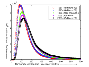
(a) Rural India

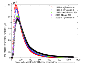
(b) Urban India

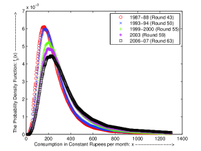
(c) Entire India

Figure 1: Kernel Density Estimate for the Expenditure Distribution in India plotted in linear scale: 1987-2007 (for Households)

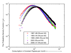
(a) Rural India

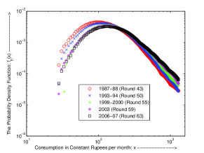
(b) Urban India

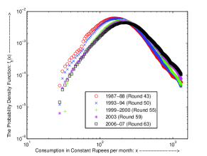
(c) Entire India

Figure 2: Kernel Density Estimate for the Expenditure Distribution in India plotted in a log-log scale: 1987-2007 (for Households)

A crucial judgment comes in the choice of the bandwidth for the kernel density plots. A rule of thumb  Pagan_Ullah ; Sala-i-Martin is to look at the standard deviation for the log of the consumption. The optimal bandwidth is given by $0.9\cdot\sigma\cdot n^{-1/5}$, where $\sigma$ is the standard deviation of the log-consumption and $n$ is the number of sample points. The standard deviation of the log-consumption, when considered at constant rupees, is almost unchanged over time. We compute the bandwidth at 0.2847 for the rural data (Fig. 1(a)) and 0.3460 for the urban data (Fig. 1(b)). Also we have the national weights for the rural and urban Indian households from the census data . Based on that, the expenditure distribution for the entire India is plotted in (Fig. 1(c)). These plots are redrawn in the log-log scale (Fig. 2(a), 2(b), and 2(c)).

The plots reveal that there is a small rightward shift in the expenditure patterns of rural and urban consumers over time. This is commensurate with the general notion of economic growth and subsequently the understanding of economic inequality in India. We address the notion of inequality in Section VI for a quantitative investigation. Since it is a grouped data, a thick tail would imply a straight line in the right compared to the overall parabolic shape of the curve when drawn in the log-log scale. The straight line is not too obvious. Nevertheless, it should be observed that in a course grouped data the tails are not properly represented through a kernel plot. The plots based on the individuals’ average monthly consumption rather than households’ display same pattern.

IV Model : Theoretical Foundation

The preliminary investigation provides us a rough idea of the expenditure distribution. Though kernel density estimates are a great tool for visual inspection of the data suitably smoothed, proposition of a theoretical distribution is a necessary pre-requisite to model the consumption process. Moreover, a theoretical basis for the empirically viable distribution is required to gather understanding about the physical characteristic of the empirically found distribution.

Let an agent consume $\tau$ goods. All the goods are available in the market with prices $p_{1}$, $p_{2}$, …, $p_{\tau}$, respectively. The consumed quantities of these goods are denoted by $g_{1}$, $g_{2}$, …, $g_{\tau}$. The utility function anindya of the consumer could be chosen as a Cobb-Douglas function,

$$u\left(g_{1},g_{2},...,g_{\tau}\right)=g_{1}^{\delta_{1}}\cdot g_{2}^{\delta_{2}}\cdots g_{\tau}^{\delta_{\tau}},$$ (1)

where $\delta_{1}$, $\delta_{2}$, …, $\delta_{\tau}$ are parameters indicating the significance of each of the goods in the felicity function of the agent.

The consumer maximizes her utility (1) subject to the following budget constraint,

$$p_{1}\cdot g_{1}+p_{2}\cdot g_{2}+\cdots p_{\tau}\cdot g_{\tau}\leq c.$$ (2)

where $c$ is the total expenditure. The first order condition of this optimization exercise is based on the principle that the marginal utility of consumption from the $i^{th}$ good is proportional to $p_{i}$. The marginal utility of the $i^{th}$ good is,

$$mu_{i}=\frac{\partial u}{\partial g_{i}}=g_{1}^{\delta_{1}}\cdot g_{2}^{\delta_{2}}\cdots\delta_{i}g_{i}^{\delta_{i}-1}\cdots g_{\tau}^{\delta_{\tau}}=\frac{\delta_{i}\cdot u\left(g_{1},g_{2},...,g_{\tau}\right)}{g_{i}}.$$ (3)

If $\displaystyle\frac{mu_{i}}{mu_{j}}>\frac{p_{i}}{p_{j}}$ then the consumption pattern is such that marginal utility from the $i^{th}$ good is more than its price when compared to the $j^{th}$ good. Economic efficiency demands that the consumer find it suitable to consume more of the $i^{th}$ good relative to the $j^{th}$ good and consequently the marginal utility of $i^{th}$ good falls to the extent that $\displaystyle\frac{mu_{i}}{mu_{j}}$ becomes equal to $\frac{p_{i}}{p_{j}}$. Similarly if $\displaystyle\frac{mu_{i}}{mu_{j}}<\frac{p_{i}}{p_{j}}$, the consumer increases the consumption of the $j^{th}$ good and eventually the equality is restored. In equilibrium, we observe the equality when the consumer maximizes her utility. If we use this equality along with the expression of $mu_{i}$ from (3), we obtain that $\displaystyle\frac{p_{i}~{}g_{i}}{\delta_{i}}=\frac{p_{j}~{}g_{j}}{\delta_{j}}$. Moreover, this equality holds valid for any arbitrary $i$ and $j$. Therefore, the following equation is satisfied in equilibrium:

$$\frac{p_{1}~{}g_{1}}{\delta_{1}}=\frac{p_{2}~{}g_{2}}{\delta_{2}}=\cdots=\frac{p_{\tau}~{}g_{\tau}}{\delta_{\tau}}.$$ (4)

As marginal utility of each of the goods in positive amount is positive, the budget constraint (2) holds with equality in equilibrium. We additionally use (4) to obtain,

$$\begin{array}[]{c}c=p_{1}~{}g_{1}+p_{2}~{}g_{2}+\cdots p_{\tau}~{}g_{\tau}\\ =p_{1}~{}g_{1}\left(1+\frac{\delta_{2}}{\delta_{1}}+\cdots+\frac{\delta_{\tau}}{\delta_{1}}\right).\end{array}$$ (5)

Without loss of generality, we can assume that good 1 represents the basic necessities of life. The importance of each good is denoted by the corresponding parameter in the utility function. If good 1 is the pre-dominant good, compared to all the other goods put together, the sum of values of parameters $\delta_{2}$, $\delta_{3}$, …, $\delta_{\tau}$ is small compared to $\delta_{1}$. Since good 1 represent the basic necessities of life, the variance in consumption of this good is rather small across individuals and we can replace it with a constant, $\kappa$. We incorporate this in (5) to gather,

$$c=\kappa\left(1+\frac{\delta_{2}}{\delta_{1}}+\cdots+\frac{\delta_{\tau}}{\delta_{1}}\right).$$

Taking logarithm of both the sides and using the rule of approximation that $\log(1+\epsilon)\approxeq\epsilon$, where $|\epsilon|$ is sufficiently small, we arrive at,

$$\log c\approxeq\log\kappa+\frac{\delta_{2}+\delta_{3}+\cdots+\delta_{\tau}}{\delta_{1}},$$ (6)

where $\delta_{2}+\delta_{3}+\cdots+\delta_{\tau}$ is sufficiently small compared to the value of $\delta_{1}$.

According to the tastes and priorities of individuals, the values of the parameters $\delta_{2}$, $\delta_{3}$, …, $\delta_{\tau}$ differ. In general, we can treat $\frac{\delta_{2}}{\delta_{1}}$, $\frac{\delta_{3}}{\delta_{1}}$, …, $\frac{\delta_{\tau}}{\delta_{1}}$ as random variables and assume that they are identically and independently drawn from a distribution with a finite mean and finite variance. If $\tau$ is sufficiently large, we appeal to the Central Limit Theorem to conclude that $\left(\frac{\delta_{2}}{\delta_{1}}+\cdots+\frac{\delta_{\tau}}{\delta_{1}}\right)$ follows a normal distribution. From (6), it is noted that $c$ follows a lognormal distribution.

In a more general scenario, the number of goods itself is a random variable. With the assumption that $\tau$ is geometrically distributed, $c$ follows a double Pareto distribution as illustrated in DoublePareto . The double Pareto distribution has both its upper and lower tails following a Pareto distribution with different parameters (say, $\alpha$ and $\beta$) . The standard form of a double Pareto density function is given by:

$$f_{dp}(x)=\left\{\begin{array}[]{l}\frac{\alpha\beta}{\alpha+\beta}x^{\beta-1}~{}~{}~{}~{}~{}~{}\mbox{for}~{}~{}~{}0<x\leq 1\\ \\ \frac{\alpha\beta}{\alpha+\beta}x^{-\alpha-1}~{}~{}~{}~{}\mbox{for}~{}~{}~{}x>1\end{array}\right.$$ (7)

A related possibility occurs when the population is divided into two strata, comprising $\pi$ and $1-\pi$ fractions. The second fraction is the poorer section consuming only the necessary items whereas the affluent class, the first section, consumes a relatively higher number of goods – both necessary and luxury items. It is quite reasonable to assume that the total number of necessary items consumed is fixed and as explained above, the expenditure distribution for the poorer section should follow a log-normal distribution. However, the number of luxury items consumed can be treated as a random variable, so that the expenditure distribution of the affluent class can be modeled as a double Pareto confined to the upper tail, which is nothing but a Pareto distribution. This is consistent with the fact that higher end of the expenditure distribution should follow a Pareto law, similar to the income distribution. The overall expenditure distribution is then given by a mixture of lognormal and Pareto distribution. The probability density function of such a distribution is expressed as,

$$f_{m}(x)=\pi\cdot f_{p}(x)+(1-\pi)\cdot f_{ln}(x),$$ (8)

where $f_{ln}(\cdot)$ and $f_{p}(\cdot)$ are the probability density functions for the log-normal and Pareto distribution with $\pi$ as the relative weight. More explicitly,

$$\begin{array}[]{lll}f_{ln}(x)&=&\displaystyle\frac{1}{\sqrt{2\pi}\sigma~{}x}e^{-\frac{(\log x-\mu)^{2}}{2\sigma^{2}}}\\ \\ f_{p}(x)&=&\nu\displaystyle\frac{x_{0}^{\nu}}{x^{\nu+1}}\cdot 1_{x>x_{0}}\end{array}$$ (9)

where $\mu$ and $\sigma^{2}$ are the parameters associated with the log-normal distribution. It is justified to use the parameter $x_{M}=\exp{\mu}$ in our analysis, as $x_{M}$ gives the median of the log-normal distribution. It may be noted that expectation of the Pareto distribution exists if and only if $\nu>1$. The value of this Pareto exponent, $\nu$, is an important parameter along with $x_{0}$, the cut-off of the Pareto tail.

V Expenditure Distribution as a Mixture of Lognormal and Pareto Distribution

V.1 Estimation of Parameters

When we fit a mixture of lognormal and Pareto distribution to the available Indian data, there are five parameters to be estimated, namely $x_{M}$, $\sigma$, $\nu$, $x_{0}$, and $\pi$. Typically, we use the method of maximum likelihood estimation to obtain a consistent estimate. However, this is a grouped data and estimation becomes much non-standard in this context. In the absence of any universally accepted procedure, we use the following methodology with some sensitivity analysis.

Table 4: Estimates of the Mixture Distribution: Rural India ($x_{0}$ and $x_{M}$ are in rupees, and others are dimensionless parameters).

Year	Household Level					Person Level
	$x_{M}$	$\sigma^{2}$	$\nu$	$x_{0}$	$\pi$	$x_{M}$	$\sigma^{2}$	$\nu$	$x_{0}$	$\pi$
1983	94.632	0.221	2.370	223.684	0.053	90.922	0.240	2.440	230.263	0.028
1987-88	124.462	0.180	1.840	200.828	0.123	121.997	0.179	2.000	224.000	0.077
1989-90	154.007	0.151	2.120	243.914	0.154	148.413	0.162	2.684	249.103	0.123
1992	211.452	0.173	1.960	385.241	0.077	199.338	0.165	2.350	385.241	0.062
1993-94	236.040	0.158	2.100	420.000	0.092	230.904	0.158	2.340	420.000	0.077
1995-96	280.620	0.143	2.086	497.000	0.108	265.072	0.128	2.150	411.310	0.138
1997	325.708	0.170	1.580	497.000	0.108	300.366	0.148	1.850	497.000	0.123
1998	322.144	0.158	1.800	497.000	0.108	289.455	0.132	1.910	419.879	0.169
1999-00	408.299	0.135	2.090	658.000	0.138	404.237	0.135	2.180	658.000	0.092
2001-02	416.547	0.158	2.638	709.655	0.138	401.015	0.153	2.800	735.000	0.092
2002	470.596	0.153	1.770	735.000	0.092	421.576	0.134	2.047	671.638	0.123
2003	452.144	0.134	1.622	684.310	0.154	424.537	0.120	2.083	671.638	0.154
2004	470.596	0.124	1.726	696.983	0.200	441.863	0.119	2.098	684.310	0.185
2004-05	434.415	0.143	1.700	644.000	0.169	434.415	0.145	2.040	784.000	0.092
2005-06	524.7910	0.163	1.660	812.000	0.108	487.359	0.135	1.980	770.000	0.123
2006-07	553.355	0.143	1.760	849.414	0.169	537.5383	0.143	2.020	849.414	0.138

Table 5: Estimates of the Mixture Distribution: Urban India ($x_{0}$ and $x_{M}$ are in rupees, others are dimensionless parameters).

Year	Household Level					Person Level
	$x_{M}$	$\sigma^{2}$	$\nu$	$x_{0}$	$\pi$	$x_{M}$	$\sigma^{2}$	$\nu$	$x_{0}$	$\pi$
1983	138.378	0.293	2.020	284.211	0.087	123.965	0.239	2.300	273.684	0.071
1987-88	188.859	0.255	1.850	351.690	0.154	172.431	0.213	1.988	344.207	0.123
1989-90	240.087	0.255	1.420	434.000	0.108	205.203	0.188	1.669	336.724	0.169
1992	295.302	0.204	1.503	483.241	0.231	275.063	0.196	1.668	483.241	0.169
1993-94	374.278	0.258	1.717	686.000	0.123	339.000	0.239	1.940	686.000	0.092
1995-96	412.403	0.188	1.431	686.362	0.246	392.682	0.180	1.450	671.759	0.185
1997	435.285	0.184	1.400	686.362	0.292	414.470	0.184	1.420	671.759	0.215
1998	453.502	0.184	1.400	700.966	0.292	422.843	0.171	1.420	657.155	0.246
1999-00	694.367	0.264	1.670	1214.741	0.123	609.111	0.220	1.810	1038.052	0.138
2001-02	679.937	0.240	1.532	1038.051	0.246	679.257	0.258	1.468	1214.741	0.108
2002	660.502	0.178	1.508	1000.276	0.354	622.660	0.173	1.670	1000.276	0.277
2003	812.406	0.268	1.400	1351.724	0.138	693.673	0.203	1.940	1270.621	0.169
2004	804.322	0.210	1.410	1297.655	0.246	758.240	0.220	1.400	1297.655	0.154
2004-05	780.551	0.272	1.420	1274.483	0.169	699.944	0.230	1.728	1274.483	0.154
2005-06	896.053	0.272	1.400	1540.000	0.154	828.818	0.258	1.400	1540.000	0.108
2006-07	991.283	0.268	1.400	1732.138	0.169	888.914	0.249	1.557	1698.828	0.138

We consider the well-accepted $\chi^{2}$ statistic for goodness-of-fit tests. We compute this statistics, $\displaystyle\sum\frac{\left(f_{observed}-f_{predicted}\right)^{2}}{f_{predicted}}$, where $f_{observed}$ is the observed frequency of the data points in a class and $f_{predicted}$ is the expected frequency of the data points as predicted by the fitted distribution and the summation is considered over all the classes. The underlying parameters determine $f_{predicted}$; therefore by changing the values for the parameters, we can change the value of the $\chi^{2}$ statistics. We minimize this statistics with respect to the values of the five parameters by simultaneous movement of the parameters in the parameter space. In other words, we maximize the $p$-value of the test for the null hypothesis which states that the theoretical distribution is the fitted one.

The most sensible thing to work with the expenditure data is to use the expenditure of a household and find the effective average expenditure per person in that household. It is implemented by finding the number of members in some sort of “equivalence scale” considering the number of adults and ages of the minor members in that household. The data are too crude to go for this. We have only the average number of households and average number of persons available for each class. Therefore, we carry out two estimates with this data-set – one involving the number of households in each expenditure bracket and the other with the number of persons in each expenditure bracket. The estimates for the various years with the rural population are reported in Table 4 and those with the urban population are tabulated in Table 5.

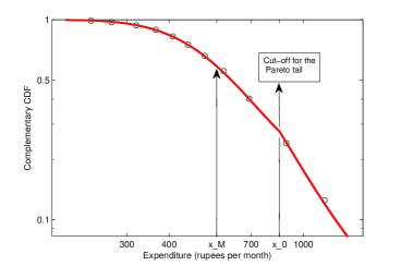
Figure 3: The Complementary CDF of the data and the fitted mixture distribution plotted in a log-log scale for the rural households (RH)for 2006-07. The circles represent the data points and the line represents the fitted distribution, which is a mixture of lognormal and Pareto.

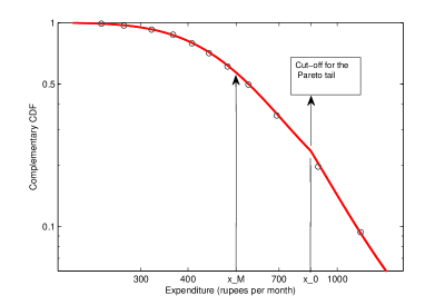
Figure 4: The Complementary CDF of the data and the fitted mixture distribution plotted in a log-log scale for the rural persons (RP) for 2006-07. The circles represent the data points and the line represents the fitted distribution, which is a mixture of lognormal and Pareto.

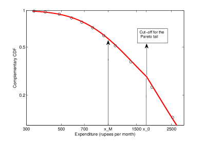
Figure 5: The Complementary CDF of the data and the fitted mixture distribution plotted in a log-log scale for the urban households (UH) for 2006-07. The circles represent the data points and the line represents the fitted distribution, which is a mixture of lognormal and Pareto.

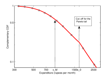
Figure 6: The Complementary CDF of the data and the fitted mixture distribution plotted in a log-log scale for the urban persons (UP) for 2006-07. The circles represent the data points and the line represents the fitted distribution, which is a mixture of lognormal and Pareto.

For the rural sector, the estimated value of $x_{M}$ falls between 90.92 and 553.36; whereas for the urban sector, estimated value of $x_{M}$ is in the range of 123.97 to 991.28. It is usually the case that the urban sector has a higher mean compared to its rural counterpart. Also, there is a clear trend of this parameter over time. We discuss the variation of $x_{M}$ over time in subsection V.5. As far as the estimate of $\sigma^{2}$ is concerned, its value lies in the interval $(0.12,~{}~{}0.24)$ for the rural population and in the range of 0.17 to 0.29 for the urban populace. Clearly, there is a larger variation in income among urban population relative to the rural sector. The Pareto tail starts at $x_{0}$ and it signifies the reach of the Pareto tail or the minimum expenditure level for consuming some luxury items. $x_{0}$ is increasing over time starting at the value of 200.83 to 849.41 among the rural population. The trend is very similar in urban sector – the value of $x_{0}$ varies within the range of 273.68 to 1732.14. The slope of the Pareto tail is described by $\nu$, whose range varies between 1.4 to 2.8. The rural sector has comparatively larger values indicating a smaller inequality in the upper segment of the population. $\pi$ represents the size of the Pareto tail or equivalently the proportion of population consuming luxury items. It varies over a wide range of 3-35%. However, if we ignore the extreme outliers, we find that it is mostly in the range of 10-20%. The complementary CDFs of the data for the year 2006-07 and the fitted mixture distribution are shown in Fig.3, Fig.4, Fig.5 and Fig.6.

V.2 Goodness-of-fit Test for the Mixture Distribution

To test our fitted statistical model independently, we employ the Kolmogorov-Smirnov (KS) statistic KS , which is a standard measure to quantify $D$, the distance between the two probability distributions with CDFs $F_{1}(\cdot)$ and $F_{2}(\cdot)$. Mathematically, the KS statistics is:

$$D=\underset{x}{\sup}|F_{1}(x)-F_{2}(x)|.$$ (10)

Table 6: Goodness-of-fit Tests of the Mixture Distribution: Rural India

Year	Household Level				Person Level
	$\chi^{2}$ Test		KS Test		$\chi^{2}$ Test		KS Test
	Statistic	p-value	Statistic	p-value	Statistic	p-value	Statistic	p-value
1983	3.0636	0.9960	0.0040	1.0000	9.3731	0.6730	0.0184	0.5950
1987-88	6.2349	0.9520	0.0195	0.9640	4.6913	0.9820	0.0198	0.7010
1989-90	6.1608	0.9710	0.0086	0.9990	6.8004	0.9530	0.0210	0.8020
1992	2.9581	1.0000	0.0095	1.0000	1.6625	1.0000	0.0097	1.0000
1993-94	0.6824	1.0000	0.0058	1.0000	1.6977	1.0000	0.0168	0.9900
1995-96	2.9031	1.0000	0.0160	0.9920	2.1251	0.9930	0.0097	1.0000
1997	5.4394	0.9850	0.0106	1.0000	6.7092	0.9710	0.0118	0.9950
1998	3.3407	0.9970	0.0187	0.9900	4.0142	0.9930	0.0087	1.0000
1999-00	2.8418	1.0000	0.0107	1.0000	2.1634	0.9940	0.0130	0.9940
2001-02	7.6461	0.9210	0.0114	0.9910	12.1979	0.7340	0.0133	0.9820
2002	3.0339	1.0000	0.0151	0.9960	1.9962	1.0000	0.0127	0.9930
2003	2.7482	1.0000	0.0165	0.9890	5.0211	0.9810	0.0190	0.9050
2004	2.9445	1.0000	0.0079	1.0000	6.9836	0.9430	0.0157	0.9770
2004-05	2.6664	1.0000	0.0072	1.0000	1.4993	1.0000	0.0088	1.0000
2005-06	3.2393	0.9950	0.0075	1.0000	3.0981	0.9980	0.0153	0.9950
2006-07	3.6661	0.9930	0.0095	0.9990	3.1909	0.9860	0.0074	0.9990

Table 7: Goodness-of-fit Tests of the Mixture Distribution: Urban India

Year	Household Level				Person Level
	$\chi^{2}$ Test		KS Test		$\chi^{2}$ Test		KS Test
	Statistic	p-value	Statistic	p-value	Statistic	p-value	Statistic	p-value
1983	9.8138	0.6270	0.0111	0.9200	6.8690	0.8610	0.0102	0.9500
1987-88	2.7907	1.0000	0.0106	0.9800	2.4100	1.0000	0.0123	0.9760
1989-90	3.5786	0.9030	0.0075	1.0000	3.2778	0.9710	0.0105	0.9820
1992	2.3625	1.0000	0.0093	0.9990	4.6247	0.9450	0.0190	0.9870
1993-94	2.3949	1.0000	0.0133	0.9770	2.0699	1.0000	0.0074	1.0000
1995-96	5.9928	0.8970	0.0186	0.9000	4.1122	0.9550	0.0115	0.9880
1997	5.3826	0.9090	0.0088	0.9990	2.6052	0.9980	0.0091	0.9910
1998	15.4850	0.6020	0.0259	0.7320	13.3152	0.6230	0.0260	0.7490
1999-00	4.1929	0.9420	0.0092	0.9880	4.4469	0.9660	0.0088	0.9910
2001-02	1.9054	1.0000	0.0071	1.0000	3.0548	0.9870	0.0121	0.9610
2002	10.5025	0.7860	0.0142	0.9820	12.0308	0.7760	0.0109	0.9750
2003	3.1115	1.0000	0.0068	1.0000	5.1039	0.8910	0.0132	0.9130
2004	6.6601	0.9110	0.0074	0.9990	4.3958	0.9730	0.0068	1.0000
2004-05	3.8926	0.9910	0.0074	1.0000	5.1956	0.9230	0.0115	0.9820
2005-06	5.5039	0.9430	0.0122	0.9880	4.7555	0.9880	0.0075	0.9980
2006-07	3.6169	0.9950	0.0100	0.9960	4.0303	0.9870	0.0069	1.0000

To perform the goodness-of-fit test, one needs to compute the empirical distribution function and the theoretical distribution function as $F_{1}(\cdot)$ and $F_{2}(\cdot)$. A standard mathematical formulation ensures that $D$ is equivalent to the maximum distance between these two CDFs in the points of the data. However, the procedure is somewhat non-standard in this case for the fact that one does not observe the individual data points, but only the classes and the class-frequencies. We can only compute the empirical distribution function at the class-limits. To test the fit using the KS statistics, we use a Monte Carlo procedure. We repeatedly simulate a sample of 1000 observations from the simulated theoretical distribution and calculate the value of the KS statistics after converting the synthetic data into a grouped one with the pre-defined class limits. The $p$-value is the proportion of such samples for which the value of the KS statistics is more than the observed value of the statistic in the original data .

The $p$-values for this goodness of fit test involving the KS statistic as well as the $\chi^{2}$ statistic are reported in Table 6 and 7 for the rural and urban populations, respectively. It is found that the $p$-values are extremely close to 1 for most of the data-sets in different years, which suggests that we can accept the proposed model at any level of significance. The $p$ values associated with the $\chi^{2}$ statistic are calculated in a similar manner which illustrate the same.

V.3 Double Pareto Distribution

Double Pareto distribution is closely related to our hypothesized distribution. We estimate the parameters of this distribution as noted in (7) with our data-set. The estimation procedure for this is similar to the previous case. The estimated parameters $\alpha$ and $\beta$ are tabulated in Table 8. Also we carry out the goodness-of-fit test with KS statistic and report the $p$-values of the test statistic for diferent cases in the same table. The relatively low values of the $p$-values often lead to rejection of the null hypothesis of the double Pareto distribution. Based on these findings, we conclude that compared to the mixture distribution, the empirical possibility of the double Pareto distribution is rather weak. This perhaps indicates that for the Indian population there is a proportion consuming on an average a fixed number of necessary items.

Table 8: Estimation and goodness-of-fit test for the Double Pareto Distribution

Year	Urban	Rural	Urban	Rural
	Households	Households	Persons	persons
	$\alpha$    $\beta$     KS    p-val.	$\alpha$    $\beta$     KS    p-val.	$\alpha$    $\beta$     KS    p-val.	$\alpha$    $\beta$     KS    p-val.
1983	1.01   0.83   0.42   0.00	1.16   1.78   0.47   0.85	1.38   1.15   0.49   0.24	0.88   2.06   0.42   0.86
1987-88	0.68   0.97   0.28   0.00	0.91   1.50   0.39   0.24	0.82   1.27   0.33   0.08	0.91   1.74   0.41   0.61
1989-90	0.98   1.04   0.40   0.00	1.36   1.21   0.58   0.01	0.88   1.52   0.38   0.26	1.35   1.40   0.53   0.01
1992	1.58   0.45   0.60   0.00	1.85   1.00   0.58   0.27	1.97   0.72   0.62   0.00	1.86   1.34   0.58   1.00
1993-94	1.01   0.71   0.42   0.00	1.17   1.48   0.47   0.21	0.96   1.13   0.39   0.00	1.29   1.48   0.50   0.15
1995-96	1.45   0.52   0.54   0.00	1.85   1.40   0.58   1.00	1.46   0.89   0.51   0.02	1.95   1.37   0.59   1.00
1997	1.23   0.82   0.43   0.01	1.83   0.88   0.56   0.54	1.68   0.66   0.56   0.00	1.70   1.15   0.54   1.00
1998	1.63   0.37   0.58   0.00	1.90   1.29   0.58 1.00	1.55   0.79   0.52   0.03	1.83   1.64   0.59   1.00
1999-00	1.07   0.66   0.46   0.00	1.25   1.49   0.49   0.19	0.98   1.07   0.40   0.00	1.21   1.82   0.50   0.44
2001-02	0.99   0.43   0.48   0.00	1.11   0.99   0.48   0.00	1.00   0.81   0.41   0.00	0.98   1.31   0.44   0.00
2002	1.32   0.37   0.59   0.00	1.33   1.42   0.50   0.35	1.27   0.76   0.50   0.00	1.41   1.52   0.52   0.43
2003	1.27   0.40   0.57   0.00	1.25   1.65   0.48   1.00	1.15   0.77   0.47   0.00	1.55   1.36   0.54   0.29
2004	0.97   0.71   0.41   0.00	1.73   1.02   0.56   0.04	0.89   1.23   0.37   0.00	1.65   1.39   0.55   0.64
2004-05	0.94   0.69   0.39   0.00	1.19   1.56   0.46   0.72	1.11   0.85   0.43   0.00	1.36   1.60   0.51   0.74
2005-06	0.82   0.82   0.35   0.00	1.53   1.02   0.54   0.01	0.67   1.15   0.29   0.00	1.74   1.32   0.57   0.32
2006-07	0.91   0.84   0.38   0.00	1.58   1.06   0.54   0.04	1.38   0.74   0.51   0.00	1.84   1.09   0.59   0.07

V.4 Comparison with Other Proposed Statistical Models in the Literature

We restrict our attention to the probability distributions of exponential, gamma, lognormal, Gompertz, and Weibull to compare with our proposed model based on the existing literature. The graphical representations show that the distribution neither follow the exponential distribution, nor Gompertz distribution. This can be explained intuitively. The exponential probability distribution, which is actually the Boltzmann-Gibbs distribution, is a characteristic feature of conserved variables such as energy or total amount of money in the population. But the expenditure variable is not conserved within the population due to transaction of money. Empirically the probability of zero expenditure must be equal to zero as every living person should have some minimum level of consumption. This is dismissive of the exponential or Gompertz distribution as far as the theoretical model is concerned.

Both the distributions of lognormal and gamma satisfy the above requirement of zero probability for zero MPCE. We have already taken into consideration of the lognormal distribution in the procedure for estimating the mixture distribution. $\pi$ is the parameter determining the relative weight of the Pareto distribution in the mixture. If this parameter of interest assumes the value of zero, we indeed end up with a pure lognormal distribution. However, this is not the case with our estimates in any year with any section of the population. We reject both the gamma distribution and the lognormal distribution for the data set in its entirety as the goodness-of-fit test gives p-values of the order of $10^{-3}$ and $10^{-4}$ respectively. Moreover, as far as Weibull distribution is concerned, testing of the model with the estimated values of the parameters yield $p$-values to be zero evidently implying the rejection of this distribution also.

V.5 Trends of the parameters over time

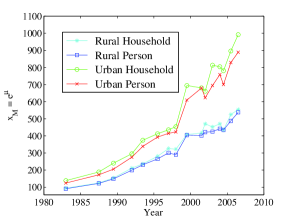
(a) Variation of $x_{M}$ over time

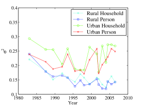
(b) Variation of $\sigma^{2}$ over time

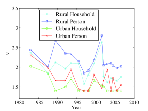
(c) Variation of $\nu$ over time

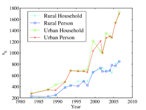
(d) Variation of $x_{0}$ over time

Figure 7: Variation of $x_{M}$ and variance $\sigma^{2}$ as well as Pareto exponent $\nu$ and Pareto cut-off value $x_{0}$ over time

It is interesting to examine if the expenditure distribution is static over time. We analyze this through the trend of the parameters of our fitted statistical model for the expenditure distribution. We plot these variations in Fig. 7. It is clear from the table that the cut-off value $x_{0}$ of the Pareto distribution is gradually increasing in time for both the rural and urban populations. It is expected for two reasons. First, the nominal incomes are growing because of inflation and if $x_{0}$ lies in certain range of quantile values of the expenditure distribution, the value of $x_{0}$ will rise over time. Secondly, the Kernel density plot reveals a slow shift of the real expenditure towards right over time due to economic growth. This causes the value of $x_{0}$ to augment without any fundamental change in the distribution over time.

We observe the movement of estimates of other parameters such as, $x_{M}$, $\sigma^{2}$, and $\nu$ over time in Fig. 7. We find that the mode of the log-normal distribution, $x_{M}$, gradually increases with time, but the variance $\sigma^{2}$ seems to possess a mild decreasing trend over time. The variance $\sigma^{2}$ denotes the inherent inequality in the expenditure distribution, which actually represents the inequality in the expenditure for the necessary goods. However, the Pareto exponent $\nu$ represents the inequality in the expenditure for the luxury items whose values are found to be varying periodically with an apparent slow decreasing trend.

To measure these observations quantitatively, we perform the least square regression of the various parameters on a linear polynomial of time $t$ with $\beta_{j}$ as the slope over time for the relevant parameter – $j=m,~{}s,~{}n,~{}x,~{}p$ for the parameters of $x_{M}$, $\sigma^{2}$, $\nu$, $x_{0}$, and $\pi$ respectively. For example, the equation for $x_{M}$ at time $t$ is

$$\begin{array}[]{ccc}x_{M}&=&\alpha_{m}+\beta_{m}\cdot t+\epsilon_{m},\\ \end{array}$$

where $\epsilon_{m}$s are the Gaussian white noise term associated with the regression equation. We then test for $H_{0}^{j}$:   $\beta_{j}=0$ against the alternative hypothesis of $H_{1}^{j}$:  $\beta_{j}\neq 0$ for $j=~{}m,~{}s,~{}n,~{}x,~{}p$. The estimates of $\beta_{j}$ ($j=~{}m,~{}s,~{}n,~{}x,~{}p$) along with the $p-$values of the performed tests are tabulated in Table 9. One could talk of non-linear trend instead of linearity. However, fitting a higher degree polynomial of $t$ does not qualitatively alter the results in any manner.

Table 9: Estimates of $\beta_{j}$s and p-value for the test of $\beta_{j}=0$ against a two-sided alternative

Types	Urban	Rural	Urban	Rural
	Households	Households	Persons	Persons
Estimated $\beta_{m}$	32.6635	17.9736	29.9158	17.0320
p-value for $\beta_{m}$=0	0.0000	0.0000	0.0000	0.0000
Estimated $\beta_{s}$	-0.0004	-0.0023	0.0009	-0.0032
p-value for $\beta_{s}$=0	0.7799	0.0017	0.4031	0.0004
Estimated $\beta_{n}$	-0.0187	-0.0192	-0.0217	-0.0148
p-value for $\beta_{n}$=0	0.0025	0.0635	0.0168	0.1307
Estimated $\beta_{x}$	58.0599	27.9017	58.9488	28.0862
p-value for $\beta_{x}$=0	0.0000	0.0000	0.0000	0.0000
Estimated $\beta_{p}$	0.0035	0.0031	0.0018	0.0035
p-value for $\beta_{p}$=0	0.2150	0.0171	0.3662	0.0111

It is found that $p$-values are zero for the test of $\beta_{m}=0$ in both urban and rural populations. There is a significant large positive trend of the location parameter. But, the $p$-values for the test $\beta_{s}$ are bigger than 0.05 in urban areas, so that we can accept that $\beta_{s}=0$ at $5\%$ level of significance. This indicates the robustness of the scale parameters in urban areas. In the rural area, the p-value for the test $\beta_{s}=0$ is not large enough to accept the null hypothesis of no trend over time. Finally, we see that the p-values for the test $\beta_{n}=0$ are more than 5% for the rural population implying no change in the parameter value over time. For the urban population, we have to reject the null hypothesis of constancy of the parameter over time and the values suggest that there is a significant negative trend for the Pareto exponent $\nu$ over time $t$. For $x_{0}$, clearly there is a positive trend over time and the magnitude of the trend for urban population is more larger than that for the rural population.

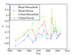
(a) Percentage of Units following Power Law

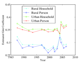
(b) Gini Coefficient

Figure 8: Variation of power law tail and Gini coefficient over time

The important question is how the number of individuals from the Pareto tail is evolving over time? The proportion of individuals in the Pareto tail is determined by $\pi$. The mean size of the Pareto tail, when considered over the entire span of this sample, for rural households, rural persons, urban households and urban persons are given by 12.45, 11.23, 19.59, and 15.73 percent, respectively. Fig. 8(a) illustrates the proportion of Indian households and persons in the Pareto tail both in the urban and the rural sector. Our estimate implies that an astonishing 10-20$\%$ of the population from the upper tail follow the Pareto law. More precisely, in the case of personal income distribution only a small fraction of the population, typically in the range of 1 to 5%, follow usa1 the Pareto law. It is certainly an interesting observation to find the discrepancy of income and expenditure distributions. This discrepancy can be explained by our interpretation of $\pi$ as the fraction of the population consuming luxury items. The larger value of $\pi$ implies this percentage corresponding to the expenditure for luxury items to be relatively high which is quite understandable. To check that whether it is evolving over time we fit a linear trend with time ($\alpha_{p}+\beta_{p}\cdot t$) for the estimates of $\pi$ for different years and test the null hypothesis of slope of the fitted line being zero. The result as tabulated in Table 9 shows that while for rural households and persons, the Pareto tail is growing over time, there is no such evidence for their urban counterparts.

It is noted that among all the parameters, those which have the larger contribution to the mean of the expenditure distribution such as $x_{0}$ and $x_{M}$ increases over time but the other parameters, which contribute to the variance or underlying inequality of the expenditure distribution, namely $\sigma$, $\nu$ and $\pi$, are comparatively robust with respect to time in both urban and rural areas. From this we may infer that the variation or the inequality in expenditure distribution of India are almost static over time, even though the mean expenditure level of India increases gradually with time in rural and urban areas.

VI Gini Coefficient: Inequality in Expenditure Distribution

The Gini coefficient ($G$), associated with the Lorenz curve, is a universally used measure of economic inequality. As $G$ does not depend on any underlying social welfare function, it may be used to predict the dynamics of economic inequality in the context of Indian consumer expenditure distribution. If $X$ denotes the expenditure variable with finite expectation $\mu_{x}$, density function $f(x)$ and cumulative distribution function $F(x)$, then we define the cumulative proportion of aggregate expenditure as

$$F_{1}(x)=\frac{\int_{0}^{x}u~{}f(u)du}{\mu_{x}}$$ (11)

The plot of $F_{1}$ against $F$ is called the Lorenz curve. If we indicate $x_{1},x_{2}....,x_{n}$ as the observed values of individual expenditure, then $G$ may be defined as

$$G=\frac{1}{2\mu_{x}}\frac{1}{n^{2}}\sum_{i,j}|x_{i}-x_{j}|$$ (12)

It can be shown that $G$ equals twice the area between the observed Lorenz curve and the line $x=y$, the line of perfect equality (or, the egalitarian line).

Table 10: Table for calculation of Gini coefficients

Expenditure	Proportion of	Average	Cumulative proportion	Proportion of	Cumulative Prop. of
classes	persons	expenditure	of persons	aggregate expenditure	aggregate expenditure
$z_{0}-z_{1}$	$p_{1}$	$\bar{x_{1}}$	$P_{1}=p_{1}$	$q_{1}=\frac{p_{1}\bar{x_{1}}}{\bar{x}}$	$Q_{1}=q_{1}$
$z_{1}-z_{2}$	$p_{2}$	$\bar{x_{2}}$	$P_{2}=p_{1}+p_{2}$	$q_{2}=\frac{p_{2}\bar{x_{2}}}{\bar{x}}$	$Q_{2}=q_{1}+q_{2}$
⋮	⋮	⋮	⋮	⋮	⋮
$z_{k-1}-z_{k}$	$p_{k}$	$\bar{x_{K}}$	$P_{k}=\sum_{i=1}^{k}\,p_{i}=1$	$q_{k}=\frac{p_{k}\bar{x_{k}}}{\bar{x}}$	$Q_{k}=\sum_{i=1}^{k}\,q_{i}=1$

From the data published by NSSO (Table 1), we construct Table 10 to calculate the points $(P_{i},Q_{i})$. The plot of the points $(P_{i},Q_{i})$ gives us the Lorenz Curve . Joining the points $(P_{i},Q_{i})$ using straight line, we derive a linear approximation of the Lorenz curve and calculate the area (say $A$) under the Lorenz curve using the Quadrature method for numerical integration . The estimate of $G$ is then given by $(1-2A)\times 100\%$, which can be used as a measure of the inequality of the expenditure distribution in India.

Table 11: Estimated Gini coefficient

Year	Urban	Rural	Urban	Rural
	Households	Households	Persons	persons
1987-88	37.48	32.29	35.78	30.90
1989-90	36.14	29.17	35.09	27.78
1992	34.85	29.04	34.51	28.68
1993-94	35.25	29.22	33.99	28.16
1997	35.31	29.06	35.00	29.00
1998	34.88	28.14	35.04	27.80
1999	35.25	27.05	34.20	25.95
2001-02	34.80	28.59	34.37	27.97
2002	35.32	27.23	35.03	26.38
2003	35.50	28.28	34.87	27.55
2004	33.49	32.86	33.49	31.99
2004-05	38.14	31.35	37.11	30.01
2005-06	36.40	29.02	35.67	27.81
2006-07	36.90	29.28	36.36	28.45

Table 12: Test for Trend in Gini Coefficient over Time

	Urban	Rural	Urban	Rural
	Households	Households	Persons	persons
Estimated $\alpha_{G}$	35.75	29.80	34.53	28.85
Estimated $\beta_{G}$	-0.0033	-0.0263	-0.028	-0.0218
95 $\%$ confidence intervals for $\beta$	(-0.109,0.1024)	(-0.175,0.1224)	(-0.0538,0.1098)	(-0.1628,0.1192)
$R^{2}$ statistic	0.0004	0.0122	0.0442	0.0094
F statistic	0.0046	0.1485	0.5544	0.1137
p-value for $\beta=0$	0.9471	0.7067	0.4709	0.7418
Estimated error variance $\sigma_{G}^{2}$	1.591	3.1468	0.9524	2.83

The estimated values of $G$ over time is tabulated in Table 11, whereas Fig. 8(b) shows the visual assessment of the movement of expenditure inequality over time. It shows that for almost every year, the households in the urban area have more economic inequality in the expenditure distribution compared to the households in rural population. This is also true for the case of individual expenditure distribution as well. In one particular year, 2004, the gap between the rural and the urban sector is negligible. However before and after that particular year, the difference persists. In general, the estimated Gini coefficients do not display any overall trend over the time horizon. This is tested by performing again the least square regression of the $G$’s on time variable $t$, i.e.

$$G=\alpha_{G}+\beta_{G}\cdot t+\epsilon_{G}$$

where the error term $\epsilon_{G}$ has zero expectation and finite variance. We test for $\beta_{G}=0$ (i.e. no trend) against the two-sided alternative of $\beta_{G}\neq 0$. It is found that p-value for this test is too large so that we can not reject the null hypothesis $\beta_{G}=0$ at any meaningful level. Therefore, the approximate value of $G$ is somewhat constant over time. It is some indicator of non-diminishing economic inequality after the liberalization of Indian economy in 1991 and consistent with the economic theories in general.

Long Pareto Tail and Gini Coefficient

It is interesting to note the evidence of a long Pareto tail of the expenditure distribution along with a moderate value of the Gini coefficient. However, the value of the Gini coefficient depends on the overall shape of the expenditure distribution, especially on the value of the exponent of the Pareto tail and the variance of the log-normal distribution. Therefore, this apparent contrast is perfectly reasonable.

We perform some simulation studies to verify the result. We generate one million observations from a distribution, which follows a mixture of log-normal and Pareto distributions with parameter values mimicking estimates of urban India for 2002. As an extreme case, it has a Pareto tail with $\nu=1.5$ with a high weight of 35.38% of the population. The average value of Gini coefficient in this simulation exercise is 42.68%. The estimated value of the Gini coefficient with the corresponding data is 35.32% for this case. This discrepancy is not unassailable bearing in mind the crudeness of the data to begin with. In this particular case, the top 10% and 20% of the population enjoy 38.78% and 50.62% of the total consumption, respectively. As a counter-factual, we also compute the Gini coefficient for a distribution exactly similar to our baseline case except with $\nu=1.1$. The Gini coefficient would have been an extreme 70.12% in that case. On the other hand with a $\nu$ of 2.5, it would have been 25.81%. Even in the baseline case, if we decrease $\pi$ to 15%, the Gini coefficient becomes 34.22%, a perfectly reasonable one.

As a comparative study with the previous literature, we look at the U.S. data. The estimated jpe expenditure and income distributions of U.S. for the cohort of years 1951-1955 are lognormals with comparatively higher variances ($\sigma=0.5578$ and $0.6258$ in contrast to $0.4212$ in our exercise with urban Indian data) for which the Gini coefficients are found to be 30.67% and 34.19%, respectively.

VII Discussion

This article discusses a theoretical basis for the lognormality of the consumption distribution and why it could possess a Pareto tail as well. It starts with a standard Cobb-Douglas utility function with many consumer goods and discusses the assumptions to arrive at the aggregate distribution. A lognormal distribution or a double Pareto distribution is also possible depending on the assumptions from a theoretical perspective.

As a first attempt, it captures the empirical aspects of expenditure distribution in India over the course of last three decades. The distribution is a mixture of lognormal and Pareto distribution. It shows a very long tail consisting of at least 10-20% of the population obeying the Pareto power law. In the lower end, it obeys the log-normal distribution. The goodness-of-fit tests reveal that this proposed distribution performs better compared to the other possibilities, such as double Pareto. Moreover, the Pareto tail is growing over time at least for the rural sector. Nonetheless, there is no evidence of any drastic change in economic inequality over time. Our analysis is in contrast to the finding of lognormal expenditure distribution with no recognizable Pareto tail for U.S. and U.K. jpe .

We conclude our discussion with a caveat that consumption decisions are very backbone of economic activities of a household or of an individual. For a clearer understanding of the business cycles from the econophysics point of view, it is necessary to have a model for the inter-relationship between income and expenditure distributions. An appropriate theory describing the relationship between the income distribution and the expenditure distribution will enhance our understanding of the economic process.

Acknowledgements: The authors highly appreciate the constructive suggestions of an anonymous referee.

References

- (1) V. Pareto, Cours d’economie politique, (Lausanne, 1897).
- (2) N. C. Kakwani, Income inequality and poverty, Oxford Unversity Press, published for the World Bank (1980).
- (3) M.E. J. Newman, Contemporary Physics 46 (2005) 323-351.
- (4) A. Banerjee, V M Yakovenko and T. Di. Matteo, Physica A 370 (2006) 54-59.
- (5) T. Di. Matteo, T. Aste, S.T. Hyde, Exchanges in compex networks: income and wealth distributions in The Physics of Complex Systems, eds. F. Mallamace and H. E. Stanley, IOS Press Amsterdam (2004), p. 43.
- (6) F. A. Cowell, F. H. G. Ferreira , J. A. Litchfeld, J. Income Distr. 8 (1998) 63-76.
- (7) N J Moura Jr and M B Rebeiro, Eur.Phys. J. B 67 (2009) 101-120.
- (8) D. Chotikapanich, D.S.Prasada Rao, K.K. Tang, Rev. Incom. and Wealth 53(2007) 127-147.
- (9) S. Sinha, Physica A 359 (2006) 555-562.
- (10) F. Clementi and M. Gallegati, Physica A 350 (2005) 427 438.
- (11) F. Clementi et al. Physica A 370 (2006) 49 53.
- (12) H. Aoyama et.al., Fractals 8 (2000) 293-300.
- (13) Y. Fujiwara et. al. Physica A 321 (2003) 598-604.
- (14) P. Lukasiewicz, A. Orlowski, Physica A 344 (2004) 146-151.
- (15) C. Quintano and A.D’Agostino, Rev. of Income and Wealth 52 (2006) 525-546.
- (16) A. Dragulescu and V M Yakovenko, Physica A 299 (2001) 213-221.
- (17) A. Harrison, Rev. of Econ. Studies, 48 (1981)621-631.
- (18) A. Christian Silva, V M Yakovenko, Europhys. Lett.69 (2005) 304-310.
- (19) A. Dragulescu and V M Yakovenko, Eur. Phys. J. B. 20 (2001) 585-589.
- (20) V. M. Yakovenko and J. B. Rosser, Jr.,Rev. Mod. Phys. 81, (2009) 1703 .
- (21) A. Chatterjee, B. K. Chakrabarti and S. S. Manna, Physica A 335 (2004) 155-163.
- (22) A. Chatterjee and B. K. Chakrabarti, Eur. Phys. J B 60 (2007) 135-149.
- (23) T. Mizuno et al. Physica A 387 (2008) 3931-3935.
- (24) E. Battistin, R. Blundell, and A. Lewbel, “Why Is Consumption More Log Normal than Income? Gibrats Law Revisited,” Journal of Political Economy Vol. 117, No. 6: pp. 1140-1154, Dec. 2009.
- (25) A. Jayadev Physica A 387 (2008) 270-276.
- (26) NSS Report Numbers: 387, 371A, 381, 397, 402, 440(52/1.0/1), 442(53/1.0/1),448(54/1.0/1), 454(55/1.0/2), 481(57/1.0/1), 484(58/1.0/1), 490(59/1.0/1), 505(60/1.0/1), 514(61/1.0/7), 523(62/1.0/1), 527(63/1/0/1) of National Sample Survey Organisation, Ministry of Statistics and Programme Implementation, Government of India.
- (27) Adrian Pagan and Aman Ullah, Nonparametric Econometrics, Cambridge University Press, 1999.
- (28) A.S. Chakrabarti and B. K. Chakrabarti, Physica A 388, (2009), 4151-4158
- (29) Xavier Sala-i-Martin, “The World Distribution of Income: Falling Poverty and Convergence, Period”, Quarterly Journal of Economics, Vol. 121, No. 2: 351-397, May 2006.
- (30) M. Mitzenmacher: Internet Math, 1, (2004) 305-333 .
- (31) I. M. Chakravarti, R. G. Laha, and J. Roy, Handbook of Methods of Applied Statistics, Volume I, John Wiley and Sons, (1967).