Quantum decoherence without reduced dynamics

Abstract

With a choice of boundary conditions for solutions of the Schrödinger equation, state vectors and density operators even for closed systems evolve asymmetrically in time. For open systems, standard quantum mechanics consequently predicts irreversibility and signatures of the extrinsic arrow of time. The result is a new framework for the treatment of decoherence, not based on a reduced dynamics or a master equation. As an application, using a general model we quantitatively match previously puzzling experimental results and can conclude that they are the measurable consequence of the indistinguishability of separate, uncontrolled interactions between systems and their environment.

I Introduction

One cannot overstate the practical importance of understanding quantum decoherence. The remarkable emergence of quantum engineering and the pursuit of quantum computation have resulted in the creation of entire industries relying upon the minimization of the effects of decoherence.

Less practical but perhaps more significant is the insight to be gained into the theory of fundamental processes. Many have sought a natural explanation for this experimental signature of an arrow of time for quantum systems, which have states represented theoretically by density operators with intrinsically reversible evolution in time Wheeler and Zurek (1983); Schulman (1997); Zeh (2007).

Phenomenologically, one imagines irreversible behavior to result from uncontrolled interactions between an experimental system and its environment. An arrow of time is thus usually accommodated in quantum theory by modeling the system of interest as a subsystem embedded within a quantum mechanical environment von Neumann (1955); Breuer and Petruccione (2002). While the time evolution of the environment plus subsystem is unitary, the time evolution of the subsystem alone need not be. In practice, one typically neglects memory effects of the environment Kossakowski (1972); Lindblad (1976) and models this reduced dynamics of the subsystem using a Lindblad-Kossakowski master equation.

Nature has provided us also with decaying states and scattering resonances, which are thought to be signatures of an asymmetry in time Bohm et al. (2003) even for closed systems. This time asymmetry is called intrinsic to distinguish it from irreversibility and the extrinsic arrow of time, which is consequent to environmental interactions. It is endowed at the microphysical level and is thus understood to have a different physical origin Bohm and Harshman (1998). If one demands a rigorous, theoretical unification of scattering resonances with decaying states, then one requires time evolution generated by a semigroup Bohm et al. (1997). Semigroup time evolution is a theoretical expression of microphysical time asymmetry.

Kossakowski and Rebolledo have recently begun to apply concepts from the intrinsically time asymmetric theory to the formulation of a new master equation Kossakowski and Rebolledo (2007). Their approach is based on the similarities between the energy spectra of subsystems embedded in an environment and of scattering resonances embedded in a continuum.

Here we take a different approach. There is a direct relationship between the intrinsic time asymmetry and the extrinsic arrow of time. If one chooses microphysically asymmetric time evolution, one must very carefully construct the theoretical images of quantum systems. One also finds a new correspondence between time evolution parameters and the passage of time in the physical universe. It is just this new correspondence, and not some mathematical effect, that leads automatically to predictions of decoherence for open systems.

After explaining briefly in Section II what we mean by intrinsically asymmetric time evolution, we will demonstrate in Section III how one must represent experimental systems.

In Section IV is an application. We derive a predictive probability for the measured decoherence of quantum systems undergoing Rabi oscillations. Furthermore, we match a general experimental result that has been particularly puzzling. Using our new approach, we conclude that what has been called Excitation Induced Dephasing Ramsay et al. (2010) is a consequence of the indistinguishability of separate, uncontrolled interactions between quantum systems and their environment.

II Groups and Semigroups

The theoretical image of a quantum mechanical system is an operator algebra defined in a linear scalar-product space, $\Phi$ Bohm (1993). The vectors $\phi_{n}$ span the space $\Phi$, and every linear combination of the $\phi_{n}$ can represent the state of the physical system. For simplicity, in this section let us consider a single vector, $\phi$, that satisfies the Schrödinger equation. The vector $\phi$ spans a one-dimensional subspace of $\Phi$, and this ray represents the quantum system in a pure state.

For the scalar-product space, $\Phi$, one has historically chosen the Hilbert space: $\Phi=\mathcal{H}$. With this choice, Stone and von Neumann showed Stone (1932); von Neumann (1932) that the time evolution of solutions is given generally by

$$\phi(t)=e^{-\frac{iHt}{\hbar}}\phi\,,\qquad-\infty<t<\infty.$$ (1)

To require $\phi\in\mathcal{H}$ is to constrain $\phi$, just as one constrains the general solutions of any differential equation by enforcing proper behavior at the boundaries. For this reason, one calls $\phi\in\mathcal{H}$ a choice of boundary conditions.

The time evolution in (1) can be described by the one-parameter group of unitary operators

$$U(t)=e^{-\frac{iHt}{\hbar}}\,,\qquad-\infty<t<\infty.$$ (2)

For every evolution, $U(t)$, there exists the inverse, $U(t)^{-1}$, given by $U(t)^{-1}=U(-t)$. This means that $U(-t)\phi$ is the time-reversed version of $U(t)\phi$, and that both are solutions of the Schrödinger equation. The resulting dynamics is intrinsically symmetric in time.

One often chooses state vectors from a different scalar-product space Dirac (1958), though usually without realizing it. When using Dirac kets ($|E\rangle$, $|\vec{x}\rangle$, etc.) with continuous spectra of eigenvalues, one has chosen $\phi\in\mathcal{S}\subset\mathcal{H}$, where the Schwartz space, $\mathcal{S}$, is a subset of $\mathcal{H}$ Bohm (1993).

Though they are measured differently, one typically assumes that scattering resonances are physically equivalent to decaying states. To find a rigorous theory in which the two can be considered also mathematically equivalent, one must constrain the state vectors even further Bohm et al. (2008):

$$\textrm{set of possible states }\{\phi\}=\Phi_{-}\subset\mathcal{H}\subset\Phi^{\times}_{-},$$ (3)

where $\Phi_{-}$ denotes the Hardy space of the lower complex semiplane, and $\Phi^{\times}_{-}$ is its dual. Note that, in practice, (3) is not a limiting restriction. Any vector in the Hilbert space can be approximated with arbitrary precision by vectors in the Hardy space Bohm and Gadella (1989). This section contains only a sketch, and for details the interested reader is referred to Bohm et al. (2006); Gadella (1983); Bohm et al. (2003) and and the numerous references therein.

The only mathematical consequence of (3) we shall consider here is that solutions of the Schrödinger equation become Bohm et al. (2006)

$$\phi(t)=e^{-\frac{iHt}{\hbar}}\phi\,,\qquad 0\leq t<\infty.$$ (4)

Note the lower bound on the time parameter. This is no longer time evolution given by the unitary group of (2). The time evolution is instead given by the one-parameter semigroup of operators,

$$U(t)=e^{-\frac{iHt}{\hbar}}\,,\qquad 0\leq t<\infty.$$ (5)

Being a semigroup means that the inverse, $U(t)^{-1}$, of any element, $U(t)$ with $t>0$, does not exist. In other words, the time-reversed version of $U(t)\phi$ is no longer an available solution of the Schrödinger equation. This dynamics is intrinsically asymmetric in time Bohm and Harshman (1998). From a choice of boundary conditions, asymmetric time evolution is endowed at the microphysical level and is independent of any interaction of a system with its environment.

The use of semigroups is not new to physics. First, expert readers will notice that (5) is not the semigroup often assumed for the family of dynamical maps for a reduced density matrix Breuer and Petruccione (2002). It has also been suggested in the past that one might describe relativistic, unstable particles using representations of the Poincaré semigroup Schulman (1970); Comi et al. (1975); Alicki et al. (1986); Exner (1983).

III Appearance of Decoherence

With our choice of boundary conditions (3), and thus the microphysical time asymmetry, comes a handful of consequences affecting the representation of experimental systems by their theoretical images. For open systems, predictions of decoherence follow automatically from standard quantum mechanics.

III.1 Coordinates and Parameters

In a recent review of time in quantum mechanics Zeh (2009), Zeh explains that, for the non-relativistic theory, one identifies the parameter $t$ in the Schrödinger equation with “Newton’s absolute,” or coordinate, time. Because in the master equation formalism, one models experimental systems as subsystems of arbitrarily large environmental systems also evolving in time, consistency requires one to identify $t$ as such.

In some cases, however, it is known that such an identification can be problematic. For instance, to formulate a sensible version of the time-energy uncertainty relation, one must distinguish between “external time,” which is measured by laboratory clocks, and “intrinsic time,” which parametrizes the dynamical evolution of experimental systems Busch (2008).

We will demonstrate that the correct application of the intrinsically time asymmetric theory requires one to distinguish between external and intrinsic time. What is called external time in Busch (2008) we will represent with time coordinates. Time coordinates are the time part of the space-time coordinates. They are physically insignificant time labels for events, and their values are given by the laboratory clocks, which are not dynamically connected to experimental systems. We will label time coordinates with a tilde: $\tilde{t}$.

What is called intrinsic time in Busch (2008) we must identify with the $t$ in the Schrödinger equation and its solutions (4). We will represent this intrinsic time with time parameters, which parametrize the time evolution of state vectors. Time parameters always correspond to durations, and we will continue to label them with the letter $t$. In Table 1 is a reminder of the distinction we will have to make.

Name	Symbol	Description
coordinate	$\tilde{t}$	$\begin{array}[]{l}\textrm{time labels for events;}\\ \textrm{marked by clocks}\end{array}$
$\begin{array}[]{l}\textrm{semigroup}\\ \textrm{time parameter}\end{array}$	$t$	$\begin{array}[]{l}\textrm{parameter for Schr\"{o}dinger}\\ \textrm{equation and solutions }\eqref{asym_states}\end{array}$

Table 1: Time coordinates and parameters.

Considering the time asymmetric boundary conditions, that one must distinguish carefully between coordinates and parameters is obvious because possible values of $t$ and $\tilde{t}$ are no longer chosen from the same interval:

$$t\in[0,\infty)\qquad\textrm{and}\qquad\tilde{t}\in(-\infty,\infty).$$ (6)

In what follows, we will assume that one can infer from measurement or from a preparation procedure the nature of a density operator meant to represent the state of a physical system. Measurements and preparations are performed in the coordinate time, $\tilde{t}$, of the laboratory, so this inferred density operator is also a function of $\tilde{t}$. Because only time durations are significant, we will call it $\rho(\tilde{t}-\tilde{t}_{prep})$, where $\tilde{t}_{prep}$ is the time coordinate value when the state of the system is prepared (see below.)

Any density operator written as $\rho(t)$ is understood to be a function of the time parameter, $t$, of theory. It is calculated using standard quantum mechanics. And as explained below, for a given system one cannot always equate $\rho(\tilde{t}-\tilde{t}_{prep})$ with $\rho(t)$. To summarize,

Calculated		Inferred from measurement
$\rho(t)$		$\rho(\tilde{t}-\tilde{t}_{prep})$

III.2 Preparation Time and $t=0$

In the theory, there is now a distinguished value, $t=0$, of the parameter used in (4) to parametrize the time evolution of state vectors. This distinguished value of time is a mathematical feature that is phenomenologically significant and identifiable in comparisons with experimental data.

One defines a physical observable by a prescription for how it is to be measured. In the theory, one represents observables with linear operators in a space $\Phi$ Bohm (1993). In the Schrödinger picture, the Born probability to find the observable $\Lambda=|\psi\rangle\langle\psi|$ in the state $\rho(t)=|\phi(t)\rangle\langle\phi(t)|$ is

$$\mathcal{P}_{\Lambda}\big{(}\rho(t)\big{)}=\mathrm{Tr}\big{(}\Lambda\,\rho(t)\big{)}=|\langle\psi|\phi(t)\rangle|^{2},\qquad 0\leq t<\infty.$$ (7)

Here the time evolution comes from (4), and the calculated probability compared with experimental measurements exists only for $0\leq t<\infty$.

For any experimental system present in a laboratory, there is also a special time: the coordinate value of the preparation time, $\tilde{t}_{prep}$. It is the time on the clock at which the state of that system has been prepared such that it is representable by, say, $\rho(t)$. It is also the time after which a detector can possibly register an observable Bohm (1999):

$$\textrm{the observable represented by }\Lambda$$

$$\textrm{is registered at }\tilde{t}\geq\tilde{t}_{prep}.$$ (8)

Comparing (III.2) with (7), one identifies the semigroup time parameter value $t=0$ of the theory with the time coordinate corresponding to the preparation of the state of an experimental system, $\tilde{t}_{prep}$:

Theory		Physical Identification
$t=0$	$\Leftrightarrow$	$\begin{array}[]{c}\textrm{preparation time of the state}\\ \textrm{of the experimental system}\end{array}$

For non-relativistic applications, then, the relation between coordinates and parameters is trivial. For a measurement performed at the duration $\tilde{t}-\tilde{t}_{prep}$ after preparation, one has

$$t\Leftrightarrow\tilde{t}-\tilde{t}_{prep}.$$ (9)

By causality, $\tilde{t}\geq\tilde{t}_{prep}$, and one cannot contradict what is in (6).

III.3 Experimental Ensembles

The results of quantum mechanical calculations are probabilities meant to be compared with averages over many identical measurements performed on identically prepared, experimental systems Dirac (1958). For actual experiments, of course, one replaces the notion of “identical” with something like “as similar as possible.” By ensemble, then, we refer to the collection of such identically prepared, experimental systems meant to undergo measurement. This is the usual understanding of ensembles, but we emphasize that we have no comment on the Ensemble Interpretation Ballentine (1970) of quantum mechanics. Nor will we reference another level of abstraction in which one imagines an ensemble of state vectors Pearle (1989) or of wave functions Zeh (2007).

While a density operator represents in principle the state of a single member as well as the state of the entire ensemble, a measurement on just one member alone is useless. An ensemble always exists for any quantitatively useful experiment.

Because of our identification of the parameter value $t=0$ with the time coordinate corresponding to the preparation of the state of an experimental ensemble, if $\rho(t)$ is to represent the state of all members of an experimental ensemble, then we require the following rule:

Rule for the application of theory

 
Every member of the ensemble, at the moment it is prepared such that it is representable by the density operator $\rho(t)$, is represented by that operator at the parametric time zero, $\rho(t=0)$, regardless of the coordinate time in the lab at which the preparation occurs.

This rule is already followed in the reduction of experimental data. This is especially clear in dynamical experiments performed repeatedly on single members of an ensemble Nagourney et al. (1986); Bergquist et al. (1986); Sauter et al. (1986); Peik et al. (1994); Meekhof et al. (1996); Brune et al. (1996); Petta et al. (2005). Because the rule is followed when reducing data, its appearance in the theory is quite natural.

III.4 Theoretical Image of an Open System

To understand why predictions of decoherence follow for open systems, consider a hypothetical sequence of three events pictured in the timeline in Figure 1:

1. A physicist prepares the state of $N$ members of an experimental ensemble at, according to the laboratory’s clock, $\tilde{t}_{prep}$. Depending on the experiment, of course, individual members of the ensemble may have different values of $\tilde{t}_{prep}$. In some experiments, these different values are recorded as “time stamps.”

2. After a duration of $\tilde{t}-\tilde{t}_{prep}=3\,\textrm{s}$, something uncontrolled (and not directly known) perturbs some members of the ensemble.

3. After the uncontrolled occurrence, the system evolves undisturbed until finally, at $\tilde{t}-\tilde{t}_{prep}=8\,\textrm{s}$, the physicist performs an active measurement.

Because of the uncontrolled occurrence in Figure 1, the system is called an open system. One can always generalize it, but for our purposes, this very simple example suffices.

Figure 1: Schematic timeline for an open quantum system.

To construct the theoretical image of this sequence, standard quantum mechanics requires the two closed systems pictured in Figure 2. The vectors $\phi_{n}$ span the space $\Phi_{\phi}$, and they can describe the state of the experimental system of interest. The vectors $\chi_{n}$ span $\Phi_{\chi}$, and they can describe the state of the uncontrolled system. By definition, any density operator defined in $\Phi_{\phi}$ can describe the state of the system of interest and of nothing external to it.

Figure 2: The extent of two closed systems.

Assume that the physicist prepares the ensemble of size $N$ to be in a pure state. In the theory, one then represents the state of the ensemble with an operator projecting into a one-dimensional subspace of $\Phi_{\phi}$ spanned by, say $\phi_{1}$. Before any uncontrolled experimental occurrence, i.e., for $\tilde{t}-\tilde{t}_{prep}<3\,\textrm{s}$ in Figure 1, the appropriate density operator at $\tilde{t}$ is

$$\rho(\tilde{t}-\tilde{t}_{prep})\Leftrightarrow\rho_{\phi}(t)=U(t)|\phi_{1}\rangle\langle\phi_{1}|U^{\dagger}(t).$$ (10)

In (10), the identification $t\Leftrightarrow\tilde{t}-\tilde{t}_{prep}$ is implicit.

If the uncontrolled event in Figure 1 does not coherently affect the entire ensemble, it affects only a subset of size $m$. And by definition, the uncontrolled occurrence cannot be described by the (closed) dynamics of the system of interest. The state of the $m$ affected members of the ensemble simply ceases to be representable by $\rho_{\phi}(t)$. Instead, one must represent their state with a new operator, $\rho_{\chi}(t)$, which is in general defined in a different space, $\Phi_{\chi}$. And according to the rule above, one must initially represent the state of the affected subset with $\rho_{\chi}(t=0)$. By preparing (passively) the state anew, the uncontrolled event resets the time parameter, $t$. This is noted in the bottom of Figure 1.

The state of the unaffected $N-m$ members remains representable by $\rho_{\phi}(t)$. For $\tilde{t}-\tilde{t}_{prep}\geq 3\,\textrm{s}$,

$$\rho(\tilde{t}-\tilde{t}_{prep})\Leftrightarrow a_{1}\,\,\rho_{\phi}(t_{1})+a_{2}\,\,\rho_{\chi}(t_{2}).$$ (11)

In (11), $a_{1}$ and $a_{2}$ are weights that will depend on $N$ and $m$, as well as on the nature of the physical systems.

Note that $\rho_{\phi}(t)=\rho_{\chi}(t)$ is possible but certainly not required. And even if they are equal, $\rho(\tilde{t}-\tilde{t}_{prep})$ in (11) will represent a mixed state because $t_{1}\neq t_{2}$ for any given value of the coordinate $\tilde{t}$ (see Figure 1.)

If $\Phi_{\phi}\neq\Phi_{\chi}$, then (11) may not be well defined. To treat it correctly one must eventually define how an operator defined on $\Phi_{\phi}$ might be extended or limited to the space $\Phi_{\chi}$. When $\Phi_{\chi}$ represents an uncontrolled environment, having $\Phi_{\phi}\neq\Phi_{\chi}$ will generally lead to predictions of dissipation. Further discussion can be left for another paper because, for the experiments we analyze in Section IV, from the data we will deduce that, immediately after the uncontrolled occurrence, $\Phi_{\phi}=\Phi_{\chi}$.

Now consider the time parameter for the affected subset of the ensemble. At measurement

$$8\,\textrm{s}=\tilde{t}-\tilde{t}_{prep}\neq t_{2}=5\,\textrm{s}.$$ (12)

To conclude (12), we have made use only of the definition of open quantum systems and of the intrinsic time asymmetry; our treatment of this hypothetical sequence is clearly independent of any model. The time parameter values, $t$, do not correspond simply to the passage of absolute time in the physical universe.

If the process of moving from (10) to (11) can be called “branching” of the density operator, then after multiple instances of environmental interference one has a density operator with many branches:

$$\rho(\tilde{t}-\tilde{t}_{prep})\Leftrightarrow a_{1}\,\,\rho_{\phi}(t_{1})+a_{2}\,\,\rho_{\chi}(t_{2})+\ldots\equiv\rho(\{t\}),$$ (13)

where $\{t\}$ is a set of time parameters.

A density operator for a pure state always branches into a density operator for a mixed state. This is a prediction of decoherence, which is an experimental signature of the quantum mechanical arrow of time. And though this branching is for the theory very simple, given our choice of boundary conditions it follows necessarily from the correct application of standard quantum mechanics.

One could conceivably develop this approach to decoherence without using the semigroup at all. Based upon the remarkable experiments in which single members of an experimental ensemble are repeatedly prepared and measured Nagourney et al. (1986); Bergquist et al. (1986); Sauter et al. (1986); Peik et al. (1994); Meekhof et al. (1996); Brune et al. (1996); Petta et al. (2005), from physical considerations one must already reset the time parameter to $t=0$ whenever ensemble members are actively prepared anew. But we have included the full development here because we enjoy how time asymmetric boundary conditions (3) lead automatically to the experimental signatures of irreversibility.

IV Application: Rabi Oscillations Experiments

As a test of our approach to open quantum systems, let us now analyze actual experimental systems within the framework of microphysical time asymmetry and the branching density operators. Our approach will allow us to address the indistinguishability of experimental ensemble members, and as a consequence we will find that our model compares very well with measurements.

IV.1 Rabi Oscillations

The theory of Rabi oscillations is well established Dodd (1991). Consider a two level system, with levels described by the projection operators $|g\rangle\langle g|$ representing the ground state and $|e\rangle\langle e|$ representing the excited state. When the system is prepared at $t=0$ to be in the excited state, $|e\rangle$, and it is coupled to a correctly tuned radiation field, the Born probability at $t$ to find the system in the ground state, $|g\rangle$, is

$$\mathcal{P}_{|g\rangle\langle g|}\big{(}\rho(t)\big{)}=\textrm{sin}^{2}(\Omega t)=\frac{1}{2}\big{(}1-\textrm{cos}(2\Omega t)\big{)},$$ (14)

where $\Omega$ is called the Rabi frequency. (The probability to find the system in the same state in which it was prepared is $\textrm{cos}^{2}(\Omega t)$.) These expressions are calculated for closed systems using standard quantum mechanics. The $t$ in (14) is therefore a single time parameter rather than a time coordinate or a set, $\{t\}$, of time parameters.

In actual experiments, one never measures the result in (14), because in practice, a physical system cannot be isolated from its environment. In this paper we wish to consider several very different but very clean and well-controlled experiments Meekhof et al. (1996); Brune et al. (1996); Petta et al. (2005); Cole et al. (2001); Zrenner et al. (2002); Wang et al. (2005); Ramsay et al. (2010).

In one experiment Meekhof et al. (1996), internal levels of a ⁹Be⁺ ion couple to a harmonic binding potential. Rabi oscillations occur between two of the coupled internal and vibrational levels, and the oscillations between different sets of levels are measured. In another experiment Brune et al. (1996), Rabi oscillations are observed between the circular states of a Rydberg atom coupled to a field stored in a high $Q$ cavity. In Petta et al. (2005), the Rabi oscillations are between the spin states of two electrons in a double quantum dot. In Cole et al. (2001), Rabi oscillations occur between motional states of electrons bound to shallow donors in semiconductors. These motional states mimic the levels of a hydrogen atom. In three experiments Zrenner et al. (2002); Wang et al. (2005); Ramsay et al. (2010), oscillations occur between excitation levels of electrons confined in quantum dots.

In Meekhof et al. (1996); Brune et al. (1996); Petta et al. (2005), one does not match the prediction in (14). Instead, the measured probability is fit by an appropriately damped sinusoid,

$$\mathcal{P}_{|g\rangle\langle g|}\big{(}\rho(\tilde{t})\big{)}=\frac{1}{2}\big{(}1-e^{-\gamma\tilde{t}}\,\textrm{cos}(2\Omega\tilde{t})\big{)},$$ (15)

where $\gamma$ is an experimentally determined damping factor. Dynamical measurements are made in the lab, and the $\tilde{t}$ in (15) is therefore a time coordinate. For simplicity, we have begun to set $\tilde{t}_{prep}=0$, with the understanding that $\tilde{t}$ hereafter represents a duration from $\tilde{t}_{prep}$.

In Petta et al. (2005), amplitude, offset, and phase are fit as well, because the oscillations are measured also as a function of a swept detuning voltage. In Wang et al. (2005); Ramsay et al. (2010), photocurrent is measured, and from it the decoherence of the Rabi oscillations is inferred. Numerically solving the models they fit to their data, the subsystems undergoing Rabi oscillations fit (15).

Experiments also reveal that the damping factor, $\gamma$, depends generally on the Rabi frequency, $\Omega$, regardless of the nature of the experiment. In the experiment with ${}^{9}\textrm{Be}^{+}$ ions Meekhof et al. (1996), the different levels are described by the kets $|\downarrow,n\rangle$ and $|\uparrow,n+1\rangle$, where $|\downarrow\rangle$ and $|\uparrow\rangle$ are internal states of the Be ion, and $|n\rangle$ represents vibrational Fock states. Rabi oscillations are measured for the frequencies Wineland et al. (1998); Meekhof et al. (1996)

$$\Omega_{n,n+1}=\Omega\frac{0.202\,e^{-0.202^{2}/2}}{\sqrt{n+1}}L^{1}_{n}(0.202^{2}),$$ (16)

where $L^{1}_{n}$ is the generalized Laguerre polynomial. The corresponding damping factor, $\gamma_{n}$, is measured to increase with $n$ according to

$$\frac{\gamma_{n}}{\gamma_{0}}\approx(1+n)^{0.7}.\qquad\textrm{(Measured)}$$ (17)

In the experiment Petta et al. (2005) with spin states of two electrons in a double quantum dot, the damping factor, $\gamma$, is stated to be proportional to the Rabi frequency, $\Omega$, though no mathematical relation is given.

In Cole et al. (2001); Zrenner et al. (2002); Wang et al. (2005); Ramsay et al. (2010), this dependence has been called Excitation Induced Dephasing (EID), and its cause has remained an open question. In Wang et al. (2005); Ramsay et al. (2010), the dependence of the damping factor on the Rabi frequency has been found to be $\gamma\propto\Omega^{2}$.

These results for such different experiments strongly suggest that some dependence of $\gamma$ on $\Omega$ is general and independent of experimental specifics.

IV.2 Development of a Model

Our task is to develop a single model of decoherence that reproduces (15) for systems undergoing Rabi oscillations, and, if possible, the general dependence of $\gamma$ on $\Omega$, or EID, also mentioned above. Because of the distinction between parameters, $t$, and coordinates, $\tilde{t}$, measured results made in coordinate time must be compared with probabilities calculated also in coordinate time. We will therefore call $\mathcal{P}_{\Lambda}\big{(}\rho(\tilde{t})\big{)}$, which is a function of coordinate time, the “predictive probability.” And below we will take $\Lambda=|g\rangle\langle g|$.

Using the branched density operator from (13), we have the predictive probability

$$\mathcal{P}_{\Lambda}\big{(}\rho(\tilde{t})\big{)} = \mathrm{Tr}\big{(}\Lambda\rho(\tilde{t})\big{)}\Leftrightarrow\mathrm{Tr}\big{(}\Lambda\rho(\{t\})\big{)}$$ (18)

$$= \mathrm{Tr}\big{(}\Lambda\,a_{1}\,\rho_{\phi}(t_{1})+\Lambda\,a_{2}\,\rho_{\chi}(t_{2})+\ldots\big{)}$$

$$= a_{1}\,\mathcal{P}_{\Lambda}\big{(}\rho_{\phi}(t_{1})\big{)}+a_{2}\,\mathcal{P}_{\Lambda}\big{(}\rho_{\chi}(t_{2})\big{)}+\ldots\,\,\,\,\,\,$$

The long-time behavior of the measured result in (15) is $\mathcal{P}_{|g\rangle\langle g|}\big{(}\rho(\tilde{t})\big{)}=\mathcal{P}_{|e\rangle\langle e|}\big{(}\rho(\tilde{t})\big{)}\rightarrow\frac{1}{2}$. From this we can deduce that there is no dissipation for the experimental system, and that the term $\mathcal{P}_{\Lambda}\big{(}\rho_{\chi}(t_{2})\big{)}$ in (18) ought not to introduce losses. For these clean experiments, we then hypothesize that immediately after the uncontrolled occurrence, $\Phi_{\phi}=\Phi_{\chi}$. Therefore, we want a predictive probability of the form

$$\mathcal{P}_{\Lambda}\big{(}\rho(\tilde{t})\big{)}\Leftrightarrow\sum_{m=0}^{M_{branch}}\,a_{m}\,\mathcal{P}_{\Lambda}\big{(}\rho_{m}(t_{m})\big{)}$$ (19)

where $M_{branch}$ is the number of branches. Note that we no longer require the label $\phi$ for $\rho$. This formula is deceptively simple in appearance, because, in general, the number of branches, $M_{branch}$, will depend on $\tilde{t}$, and the value of $a_{m^{\prime}}$ for a fixed $m^{\prime}$ will depend on $M_{branch}$.

The time parameter values $t_{m}$ are related unambiguously to $\tilde{t}$ via the rule in Section III.3. The $a_{m}$ will come from models.

We still require a prescription for the $\rho_{m}$. Leggett has explained Leggett (1997) that decoherence “is exactly the result of a ‘measurement’ whose result is uninspected,” and he has called this process “garbling.” Measuring a system to be in a state is equivalent to preparing that system to be in that state, so these passive measurements that garble an ensemble are also passive preparations. We will therefore assume that the effect of an uncontrolled interference event is to measure and therefore prepare anew some subset of our ensemble. And for obvious reasons, one should assume that nature does not distinguish between passive and active preparations.

A hypothesis physically equivalent to garbling is that the uncontrolled environment interacts only with energy eigenstates of the system of interest. Then, because $\Phi_{\chi}=\Phi_{\phi}$, when the uncontrolled event occurs at $t_{m}=0$, the most general form for $\rho_{m}$ is

$$\rho_{m}(t_{m}=0)=w_{m}\,\,|g\rangle\langle g|+v_{m}\,\,|e\rangle\langle e|,$$ (20)

with $w_{m}+v_{m}=1$. In (20), $w$ is a weight appropriate for ensemble members prepared passively to be in the ground state, and $v$ is a weight for ensemble members prepared in the excited state. The weights are of course independent of $t_{m}$, and their values will also come from our model.

IV.3 Predictive Probability

Given our hypotheses and deductions, the simplest reasonable and general model the author can conceive is:

1. Members of the experimental ensemble are actively prepared in the lab at $\tilde{t}=\tilde{t}_{prep}$. Again, for simplicity, we set $\tilde{t}_{prep}=0$.

2. The members of the ensemble can possibly suffer environmental interactions at the times $n\Delta\tilde{t}$, where $n=1,2,3\ldots$ As a result, some systems are passively prepared to be in either the ground state or the excited state. We will call these interactions “interference events.”

3. At every $n\Delta\tilde{t}$, there is some probability, $(1-\eta$), for a member to suffer perturbation and thereby to be prepared passively.

In the second step, we have introduced the time scale, $\Delta\tilde{t}$, of interaction with the environment.

In the third step we have introduced a parameter, $\eta$, with $0\leq\eta\leq 1$, to represent the susceptibility of ensemble members to environmental interference. As described, the parameter $\eta$ is the probability for any given member of the ensemble not to suffer interference at one of the times $n\Delta\tilde{t}$. For a perfectly isolated system, $\eta=1$.

According to this simple model, we can write a general formula for the predictive probability as more and more branches form:

$$\mathcal{P}_{|g\rangle\langle g|}\big{(}\rho(\tilde{t})\big{)}=\begin{cases}p_{0}(\tilde{t})&0\leq\tilde{t}<1\,\Delta\tilde{t}\\ p_{1}(\tilde{t})&1\,\Delta\tilde{t}\leq\tilde{t}<2\,\Delta\tilde{t}\\ \quad\vdots&\qquad\vdots\\ p_{n}(\tilde{t})&n\Delta\tilde{t}\leq\tilde{t}<(n+1)\Delta\tilde{t}\end{cases}$$ (21)

Here, every $p_{n}(\tilde{t})$ will have the form of the sum in (19), and $M_{branch}=n$.

Let us assume that a physicist identically prepares every member of the experimental ensemble initially to be in the excited state, $|e\rangle$. Because no members will have suffered environmental interference before $\tilde{t}=1\,\Delta\tilde{t}$, we have for the initial value $p_{0}(\tilde{t})=\textrm{sin}^{2}(\Omega\tilde{t})$.

At $\tilde{t}=1\,\Delta\tilde{t}$, the fraction $(1-\eta)$ of the ensemble will be passively measured and thus prepared in a new state, with new initial conditions. At this point, $M_{branch}=1$, and from (19) we have

$$p_{1}(\tilde{t})\Leftrightarrow a_{0}\,\mathcal{P}_{|g\rangle\langle g|}\big{(}\rho_{0}(t_{0})\big{)}+a_{1}\,\mathcal{P}_{|g\rangle\langle g|}\big{(}\rho_{1}(t_{1})\big{)}.$$ (22)

The first term in (22), $a_{0}\,\mathcal{P}_{|g\rangle\langle g|}\big{(}\rho_{0}(t_{0})\big{)}$, corresponds to the subset of the ensemble that passes the time $1\Delta\tilde{t}$ without suffering interaction with the environment. According to our model, it is $\eta\,\textrm{sin}^{2}(\Omega\tilde{t})=\eta\,p_{0}(\tilde{t})$. For this unperturbed subset, of course, $\tilde{t}\Leftrightarrow t_{0}$.

The second term in (22), $a_{1}\,\mathcal{P}_{|g\rangle\langle g|}\big{(}\rho_{1}(t_{1})\big{)}$, is the first branch. It corresponds to the subset of the ensemble that suffers perturbation and is thereby garbled, or passively prepared anew. According to our model, $a_{1}=(1-\eta)$.

By our prescription for the density operators, we know that $\rho_{1}(t_{1}=0)$ is fixed by the state of the perturbed subset as it is prepared at $\tilde{t}=1\Delta\tilde{t}$ by the uncontrolled event. The perturbed subset is passively measured at $\tilde{t}=1\Delta\tilde{t}$, so assuming that garbling is a fair measurement, $\rho_{1}(t_{1}=0)$ will have the form of (20) with $w_{1}=\textrm{sin}^{2}(1\,\Omega\Delta\tilde{t})=p_{0}(1\Delta\tilde{t})$ and $v_{1}=1-p_{0}(1\Delta\tilde{t})$.

Finally, with the identification $t_{1}\Leftrightarrow\tilde{t}-1\Delta\tilde{t}$ for the perturbed subset (see Figure 1), it is straightforward to find from the theory of Rabi oscillations

$$p_{1}(\tilde{t})=\eta\,p_{0}(\tilde{t})+(1-\eta)\Big{(}p_{0}(1\Delta\tilde{t})\,\textrm{cos}^{2}\big{(}\Omega\,(\tilde{t}-1\Delta\tilde{t})\big{)}+\big{(}1-p_{0}(1\Delta\tilde{t})\big{)}\,\textrm{sin}^{2}\big{(}\Omega\,(\tilde{t}-1\Delta\tilde{t})\big{)}\Big{)}.$$ (23)

This is a nice form because we can stop writing out branches and use a recursive formula for the predictive probability. For general $n$, we have

$$p_{n}(\tilde{t})=\eta\,p_{n-1}(\tilde{t})+(1-\eta)\Big{(}p_{n-1}(n\Delta\tilde{t})\,\textrm{cos}^{2}\big{(}\Omega\,(\tilde{t}-n\Delta\tilde{t})\big{)}+\big{(}1-p_{n-1}(n\Delta\tilde{t})\big{)}\,\textrm{sin}^{2}\big{(}\Omega\,(\tilde{t}-n\Delta\tilde{t})\big{)}\Big{)}.$$ (24)

Figure 3 shows the results of two sample calculations using (21) with (24).

(a) With $\eta=0.99$, we fit $\gamma/\Omega=0.05$.

(b) With $\eta=0.997$, we fit $\gamma/\Omega=0.015$.

Figure 3: The predictive probability, $\mathcal{P}_{|g\rangle\langle g|}\big{(}\rho(\tilde{t})\big{)}$, when members of the ensemble are distinguishable. For both plots, $\Omega\Delta\tilde{t}\approx 0.08$. The dots are the results of recursive calculations using (24) and (21). The solid lines are plots of the damped sinusoid (15) that fits the experimental data. Recall that $\eta$ is the probability that members will not suffer a perturbation at the times $n\Delta\tilde{t}$. Values of $\eta$ and $\Delta\tilde{t}$ were chosen for aesthetics only. These plots do look good, but our results are not yet correct. See the text.

The dots are from the recursive calculation using our model. The solid lines are plots of the decaying sinusoid in (15), which fits the experimental measurements. For both figures we have used $\Omega\Delta\tilde{t}\approx 0.08$. The results in Figure 3(a) were calculated using $\eta=0.99$ and resulted in a fitted value for the damping factor of $\gamma/\Omega=0.05$. The results in Figure 3(b) were calculated using $\eta=0.997$ and resulted in a fitted value for the damping factor of $\gamma/\Omega=0.015$. Recall that $\eta=1$ for a perfectly isolated system.

Our calculation of the predictive probability results in no frequency shift away from the Rabi frequency, $\Omega$, at early times, in agreement with experiments. (With the master equation, one predicts a frequency shift and must assume very strong driving to get rid of it. See Section IV.5.) Note, however, that our method results in a fitted damping factor, $\gamma$, that is independent of $\Omega$. Though our first attempt has been instructive, it is thus not correct. We have included this incorrect result not only because it clearly illustrates our new method, but also because the recursive structure of (24) will reappear in the correct model below.

IV.4 Predictive Probability and Indistinguishability

Consider the experiments Meekhof et al. (1996); Brune et al. (1996); Petta et al. (2005) in which one repeatedly prepares and then measures single members of the experimental ensemble. One assumes that performing a number of consecutive measurements, each done on a single member, is equivalent to performing a measurement on the same number of non-interacting, simultaneously present members of an identically prepared ensemble. This is a statement of ergodicity. And when the identically prepared members are present simultaneously, one treats them as indistinguishable. In our first model, we did not treat them so. And to enforce ergodicity, we would like to.

Though in these experiments, one can easily label any member of the ensemble with the value of the time coordinate, $\tilde{t}$, at which it was actively prepared or measured, coordinate values are always physically meaningless. The only physically significant label for identically prepared members is the duration between preparation and measurement. And, even in these experiments, one cannot in principle label any given member of an ensemble with a duration. To understand why, consider the result of a hypothetical, active measurement on any single member of an experimental ensemble:

1. At $\tilde{t}=0$ a physicist actively prepares the members.

2. At $\tilde{t}=1\Delta\tilde{t}$ subset $A$ is passively prepared to be in a mixture of the ground state and the excited state.

3. At $\tilde{t}=2\Delta\tilde{t}$ subset $B$ is passively prepared to be in a mixture of the ground state and the excited state.

4. At some time coordinate value $\tilde{t}>2\Delta\tilde{t}$ a physicist actively measures a single member to be in the ground state, $|g\rangle$.

Because of the probabilistic nature of quantum mechanics, it is impossible to distinguish if the actively measured member was in subset $A$, subset $B$, both, or neither.

In other words, if the state of an ensemble is represented by the branched density operator

$$\rho(\{t\})=a_{0}\,\,\rho_{0}(t_{0})+a_{A}\,\,\rho_{A}(t_{A})+a_{B}\,\,\rho_{B}(t_{B}),$$ (25)

then it is impossible to know to which branch any given member belongs.

One way to distribute indistinguishable ensemble members among several branches is to count different combinations of the members themselves. But we cannot use such an approach for two important reasons. The first is because quantum mechanics makes predictions for ensemble averages, and density operators simply do not follow the trajectories of individual members. The second reason is that any model based on such counting will depend on the size of the experimental ensemble. This is clearly unacceptable.

If, however, one imagines that ensemble members are labeled by the individual interference events at which they have been most recently prepared, we hypothesize that we can enforce ergodicity by treating the events themselves as indistinguishable. The resulting models will depend not on the ensemble size but instead on the number of interference events, which is exactly what we want.

When modeling experiments, one would probably use a full simulation. To maintain transparency, however, we will again search for an analytical formula. First, assume that we wish to calculate the predictive probability given that there have been $n$ chances for ensemble members to have suffered a single interference event. If interference events can possibly occur at intervals of $\Delta\tilde{t}$, the predictive probability can be written $\mathcal{P}_{|g\rangle\langle g|}\big{(}\rho(n\Delta\tilde{t})\big{)}$. Our scenario is as follows:

1. Choose a combination of time intervals (of length $\Delta\tilde{t}$) such that systems have survived only a duration of $1\,\Delta\tilde{t}$ before being passively measured.

2. Adjust the probability at $\boldsymbol{n}\boldsymbol{\Delta}\tilde{\boldsymbol{t}}$ accordingly.

3. Because the systems and interference events are indistinguishable, so are the intervals between the events. Put the intervals chosen above back into the original set.

4. Choose a combination of time intervals such that systems have survived a duration of $2\,\Delta\tilde{t}$ before being passively measured.

5. Adjust the probability at $\boldsymbol{n}\boldsymbol{\Delta}\tilde{\boldsymbol{t}}$ accordingly.

6. Put the intervals chosen above back into the original set.

7. Repeat until reaching $n\Delta\tilde{t}$.

We have again chosen to parametrize our model with a time scale, $\Delta\tilde{t}$. However, we will require a slightly different interpretation for the number parameterizing the members’ susceptibility to environmental interference. We shall now use $\beta$ (rather than $\eta$), with $0\leq\beta\leq 1$ and $\beta=1$ for a perfectly isolated system. Physically, $\beta$ will be the probability that a randomly chosen time interval will have come before an interference event. This can be better understood after equation (31).

To implement steps 1 and 4 above, we will make use of the binomial distribution,

$$b(n,k,\beta)\equiv{n\choose k}\beta^{k}(1-\beta)^{n-k}.$$ (26)

The distribution in (26) gives the probability for the occurrence of any combination, regardless of order, of $k$ events with probability $\beta$ and $(n-k)$ events with probability $(1-\beta)$. Because the distribution gives probabilities for combinations rather than permutations, with it we can treat indistinguishable interference events. Note also the normalization

$$\sum_{k=0}^{n}{n\choose k}\beta^{k}(1-\beta)^{n-k}=1.$$ (27)

Using (27) we will relate the binomial distribution to a probability.

To implement steps 2 and 5 in this model, we will once more use the rule deduced in Section III.3, to reset to $t=0$ the time evolution parameter of the density operator corresponding to members passively prepared as a result of environmental interference.

To see how the binomial weights work, let us write a simple formula for the case that individual ensemble members will have suffered only one interference event before an active measurement occurs. This will truncate our formula at a reasonable size, and we will generalize to multiple events below. The probability at $4\Delta\tilde{t}$ to find in $|g\rangle$ members that have been initially prepared at $\tilde{t}=0$ to be in $|e\rangle$ is

$$\mathcal{P}_{|g\rangle\langle g|}\big{(}\rho(4\Delta\tilde{t})\big{)} = b(4,4,\beta)\Big{(}\textrm{sin}^{2}(\Omega\,4\Delta\tilde{t})\,\textrm{cos}^{2}(\Omega\,0\Delta\tilde{t})+\textrm{cos}^{2}(\Omega\,4\Delta\tilde{t})\,\textrm{sin}^{2}(\Omega\,0\Delta\tilde{t})\Big{)}+$$ (28)

$$b(4,3,\beta)\Big{(}\textrm{sin}^{2}(\Omega\,3\Delta\tilde{t})\,\textrm{cos}^{2}(\Omega\,1\Delta\tilde{t})+\textrm{cos}^{2}(\Omega\,3\Delta\tilde{t})\,\textrm{sin}^{2}(\Omega\,1\Delta\tilde{t})\Big{)}+$$

$$b(4,2,\beta)\Big{(}\textrm{sin}^{2}(\Omega\,2\Delta\tilde{t})\,\textrm{cos}^{2}(\Omega\,2\Delta\tilde{t})+\textrm{cos}^{2}(\Omega\,2\Delta\tilde{t})\,\textrm{sin}^{2}(\Omega\,2\Delta\tilde{t})\Big{)}+$$

$$b(4,1,\beta)\Big{(}\textrm{sin}^{2}(\Omega\,1\Delta\tilde{t})\,\textrm{cos}^{2}(\Omega\,3\Delta\tilde{t})+\textrm{cos}^{2}(\Omega\,1\Delta\tilde{t})\,\textrm{sin}^{2}(\Omega\,3\Delta\tilde{t})\Big{)}+$$

$$b(4,0,\beta)\Big{(}\textrm{sin}^{2}(\Omega\,0\Delta\tilde{t})\,\textrm{cos}^{2}(\Omega\,4\Delta\tilde{t})+\textrm{cos}^{2}(\Omega\,0\Delta\tilde{t})\,\textrm{sin}^{2}(\Omega\,4\Delta\tilde{t})\Big{)}.$$

The explanation of (28) is straightforward. We need to relate the binomial distribution to the passage of time, so at every step $k$, with $0\leq k\leq n=4$, we will count the (normalized) number of combinations for arranging the $n$ time intervals such that $k$ of them came before the single interference event. This number is given by $b(n,k,\beta)$. Because possible interference events occur at increments of the time scale, $\Delta\tilde{t}$, the weight $b(n,k,\beta)$ must then be attached to any passive preparation occurring at $k\Delta\tilde{t}$.

Again, branches of a density operator form when subsets of the ensemble suffer environmental interference and are passively prepared. For a branched density operator, in each line of (28), the term multiplied by $b(n,k,\beta)$ is the Born probability for the branches formed at $k\Delta\tilde{t}$.

Consider the second line, where $k=3$, and compare to the notation in (20). The weight $w=\textrm{sin}^{2}(\Omega\,3\Delta\tilde{t})$. The weight $v=\textrm{cos}^{2}(\Omega\,3\Delta\tilde{t})$. The duration from passive preparation to $4\Delta\tilde{t}$ is then $(4-3)\Delta\tilde{t}=1\Delta\tilde{t}$, so the functions with argument $1\Delta\tilde{t}$ contain the time dependence of the Born probability of the mixed state.

Let us introduce the notation $\mathcal{P}^{(i)}_{|g\rangle\langle g|}\big{(}\rho(n\Delta\tilde{t})\big{)}$ to represent the predictive probability under the assumption that members on average will have suffered $i$ or fewer interference events before measurement. Then for general $n$,

$$\mathcal{P}^{(1)}_{|g\rangle\langle g|}\big{(}\rho(n\Delta\tilde{t})\big{)}=\sum_{k=0}^{n}b(n,k,\beta)\Big{(}\textrm{sin}^{2}(\Omega\,k\Delta\tilde{t})\,\textrm{cos}^{2}(\Omega(n-k)\Delta\tilde{t})+\textrm{cos}^{2}(\Omega\,k\Delta\tilde{t})\,\textrm{sin}^{2}(\Omega(n-k)\Delta\tilde{t})\Big{)}.$$ (29)

By simply exchanging the $\textrm{cos}^{2}(\Omega\,k\Delta\tilde{t})$ and $\textrm{sin}^{2}(\Omega\,k\Delta\tilde{t})$ terms, we calculate $\mathcal{P}^{(1)}_{|e\rangle\langle e|}\big{(}\rho(n\Delta\tilde{t})\big{)}$, which is the probability to find the ensemble members in the excited state.

In (29), we have assumed that systems will have suffered at most one interference event. To allow for the possibility of multiple events, the terms $\textrm{sin}^{2}(\Omega\,k\Delta\tilde{t})$ and $\textrm{cos}^{2}(\Omega\,k\Delta\tilde{t})$ must be replaced with new functions of $k\Delta\tilde{t}$, that predict the effects of interference events prior to the single event assumed in (29). For general $i$,

$$\mathcal{P}^{(i)}_{|g\rangle\langle g|}\big{(}\rho(n\Delta\tilde{t})\big{)}=\sum_{k=0}^{n}b(n,k,\beta)\Big{(}\mathcal{P}^{(i-1)}_{|g\rangle\langle g|}\big{(}\rho(k\Delta\tilde{t})\big{)}\,\textrm{cos}^{2}(\Omega(n-k)\Delta\tilde{t})+\mathcal{P}^{(i-1)}_{|e\rangle\langle e|}\big{(}\rho(k\Delta\tilde{t})\big{)}\,\textrm{sin}^{2}(\Omega(n-k)\Delta\tilde{t})\Big{)}.$$ (30)

In (30), the recursive structure of (21) and (24) has reappeared, but here the ensemble members and interference events are indistinguishable. Handling the possibility for more and more interference events requires the nesting of more and more summed terms into (30). These nested equations are significantly more difficult to solve than are the recursive equations used for distinguishable events.

We have written the predictive probability as a function of $n\Delta\tilde{t}$. The final step is to scale our result back to the time coordinate, $\tilde{t}$. The first moment of the binomial distribution is

$$\langle k\rangle=\sum_{k=0}^{n}{n\choose k}\beta^{k}(1-\beta)^{n-k}\,k=\beta\,n.$$ (31)

After stepping through time to $n\Delta\tilde{t}$, on average $\beta\,n$ of the intervals will have preceded the interference event number $i$. This provides us a physical interpretation of our two parameters, and to ensure that the time scales with something physical, we will need to use $\langle k\rangle\Delta\tilde{t}=\beta\,n\Delta\tilde{t}=\tilde{t}$. After a calculation of the predictive probability as a function of $n\Delta\tilde{t}$, we make the replacement

$$n\rightarrow\frac{\tilde{t}}{\beta\,\Delta\tilde{t}}\,.$$ (32)

This restricts us to non-zero values of $\beta$ and $\Delta\tilde{t}$. We have also simply interpolated between the discrete values of $n$ at which (30) is actually defined. Because our time scale is understood to be an average value, it would be inappropriate to assume for our model anything more complicated.

The predictive probability at $\tilde{t}$, assuming $i$ interference events, to find in the ground state a system initially prepared in the excited state is therefore

$$\mathcal{P}^{(i)}_{|g\rangle\langle g|}\big{(}\rho(\tilde{t})\big{)}=\mathcal{P}^{(i)}_{|g\rangle\langle g|}\big{(}\rho(n\Delta\tilde{t})\big{)},\quad n\rightarrow\frac{\tilde{t}}{\beta\,\Delta\tilde{t}}\,.$$ (33)

Numerical solution of (30) is straightforward. One can also perform the summations and find closed form expressions for the predictive probabilities. In Figure 4 we have plotted $\mathcal{P}^{(5)}_{|g\rangle\langle g|}\big{(}\rho(\tilde{t})\big{)}$, which is the predictive probability given that there have been for the average member $5$ or fewer interference events. For clean experiments, with $\beta$ close to $1$, we expect a good approximation for $i=5$. Again, the agreement with the experimentally measured damped sinusoid is very good.

Figure 4: Plot of the predictive probability, $\mathcal{P}^{(5)}_{|g\rangle\langle g|}\big{(}\rho(\tilde{t})\big{)}$, for indistinguishable ensemble members. For the dots we have used equations (30) and (33). The solid line is a plot of the damped sinusoid (15) that fits the experimental data. We have used $\Omega\Delta\tilde{t}\approx 0.7$ and $\beta=0.995$, and we have fit $\gamma/\Omega=0.039$.

As opposed to the previous results for distinguishable ensemble members, however, when we treat the interference events as indistinguishable, we find that the damping factor, $\gamma$, does in general depend on the Rabi frequency, $\Omega$, in agreement with measurements and the phenomenon called Excitation Induced Dephasing. Furthermore, in our simple model we have assumed only a time scale, $\Delta\tilde{t}$, and a parameter, $\beta$, describing the experimental system’s susceptibility to interference from the environment. It can be applied to any real system undergoing Rabi oscillations.

For $\beta$ close to $1$, the predictive probability is dominated by the terms proportional to $b(n,k=n,\beta)$. Solving the rather crude, truncated form

$$\mathcal{P}_{|g\rangle\langle g|}\big{(}\rho(n\Delta\tilde{t})\big{)}\approx\sum_{k=0}^{n}b(n,k,\beta)\textrm{sin}^{2}(\Omega\,k\Delta\tilde{t})$$ (34)

and using (33), we get

$$\mathcal{P}_{|g\rangle\langle g|}\big{(}\rho(\tilde{t})\big{)} \approx \frac{1}{4}\Big{(}2-\big{(}1-\beta(1-e^{-2i\Delta\tilde{t}\Omega})\big{)}^{\frac{\tilde{t}}{\beta\Delta\tilde{t}}}$$ (35)

$$\,\,\quad-\big{(}1-\beta(1-e^{+2i\Delta\tilde{t}\Omega})\big{)}^{\frac{\tilde{t}}{\beta\Delta\tilde{t}}}\Big{)}.$$

For small $\Delta\tilde{t}$, (35) is

$$\mathcal{P}_{|g\rangle\langle g|}\big{(}\rho(\tilde{t})\big{)}=\frac{1}{2}\Big{(}1-e^{-\gamma\tilde{t}}\,\big{(}\textrm{cos}(2\Omega\tilde{t})+\textrm{O}(\Delta\tilde{t}^{\,2})\big{)}\Big{)},$$ (36)

where

$$\gamma=2\,(1-\beta)\,\Omega^{2}\,\Delta\tilde{t}+\textrm{O}(\Delta\tilde{t}^{\,3}).$$ (37)

For $\beta\approx 1$ and $\Omega\Delta\tilde{t}\ll 1$, $\gamma$ is quadratic in $\Omega$. This matches the results in Wang et al. (2005); Ramsay et al. (2010). And when the systems are treated as indistinguishable, we require none of the typical assumptions regarding the frequency response of perturbation terms Romito and Gefen (2007); Wang et al. (2005); Ramsay et al. (2010); Mogilevtsev et al. (2008).

The same model is general enough to apply also to the system in Meekhof et al. (1996), and with it we fit the measured relation (17) between $\gamma$ and $\Omega$. Figure 5 is the result of fitting the damping factor, $\gamma_{n}$, to $\mathcal{P}^{(5)}_{|g\rangle\langle g|}\big{(}\rho(\tilde{t})\big{)}$, calculated with the sequence of frequencies in (16) and with $\Omega_{0}\Delta\tilde{t}\approx 0.2$. (The exponent can be shifted by choosing different time scales.) Unfortunately, we are limited by computational resources to $n\leq 6$.

Figure 5: Matching the experimental results for the ratio of damping factors, $\frac{\gamma_{n}}{\gamma_{0}}$. The large dots result from our theoretical calculation of the predictive probability using (30) and (33). The solid line is the experimentally measured relation, $(1+n)^{0.7}$. To indicate a scale for the exponent, the thin dashed line is a plot of $(1+n)^{0.8}$, and the thin dotted line is a plot of $(1+n)^{0.6}$.

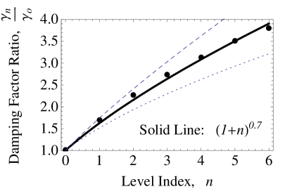
Figure 5 shows a very good quantitative agreement with experiment (17), and again we have not required any experimentally specific assumptions. Our study indicates that the decoherence measured in Meekhof et al. (1996) results from environmental interference having a characteristic frequency of $\approx 5\Omega_{0}$.

Finally, we can conclude that a dependence of $\gamma$ on $\Omega$, or EID, is indeed general, as suggested by experiment, and that it is a measurable effect of the indistinguishability of separate, uncontrolled interactions between quantum systems and their environment.

IV.5 Comparison With the Standard Program

In the standard decoherence program, one treats these experiments using the decoherence master equation. It is the method of choice when one works without time asymmetric boundary conditions and when one identifies $t$ with coordinate time. The generic solution of the master equation describing a system undergoing Rabi oscillations and on resonance is Breuer and Petruccione (2002)

$$\mathcal{P}^{ME}_{|g\rangle\langle g|}(t)=\frac{4\Omega^{2}}{\Gamma^{2}+8\Omega^{2}}\big{(}1-e^{-3\Gamma t/4}(\textrm{cos}\,\mu t+\frac{3\Gamma}{4\mu}\textrm{sin}\,\mu t)\big{)}.$$ (38)

To match our convention, we have added a factor of $2$ to the definition of Rabi Frequency in Breuer and Petruccione (2002). In (38), $\mu=\sqrt{4\Omega^{2}-\big{(}\frac{\Gamma}{4}\big{)}^{2}}$. Unless a specific environmental interaction has been assumed, $\Gamma$ is the spontaneous emission rate for the system in its excited state. It is a constant, independent of the Rabi frequency.

A significant shift from the Rabi frequency, $\Omega$, is not observed in experiments, however, so one must assume very strong driving: $2\Omega\gg\Gamma/4$. The limit of (38) is then

$$\mathcal{P}^{ME}_{|g\rangle\langle g|}(t)=\frac{1}{2}\big{(}1-e^{-3\Gamma t/4}\textrm{cos}\,2\Omega t\big{)}.$$ (39)

One can see immediately why the measured results have been puzzling. For general calculations, the solution (39) of the master equation predicts for the experiment in Meekhof et al. (1996)

$$\frac{\gamma_{n}}{\gamma_{0}}=1,\qquad\quad\textrm{(Master equation)}$$ (40)

and that $\gamma$ is independent of $\Omega$.

In the hope of matching experiment, one typically assumes a detailed form for the interaction operators. For the experiment in Meekhof et al. (1996), in which (17) was measured, several such studies have been carried out Schneider and Milburn (1998); Murao and Knight (1998); Bonifacio et al. (2000); Di Fidio and Vogel (2000); Serra et al. (2001); Budini et al. (2002, 2003). None of these studies, however, has resulted in an agreement as quantitatively good as that in Figure 5.

Furthermore, the models for decoherence in Schneider and Milburn (1998); Murao and Knight (1998); Bonifacio et al. (2000); Di Fidio and Vogel (2000); Serra et al. (2001); Budini et al. (2002, 2003) have necessarily been highly tuned. They are thus not applicable to the other types of experiments Petta et al. (2005); Cole et al. (2001); Zrenner et al. (2002); Wang et al. (2005); Ramsay et al. (2010). And, with the exception perhaps of Bonifacio et al. (2000), they suggest that a dependence of $\gamma$ on $\Omega$ is not general, in disagreement with measurements. Similarly, the models Romito and Gefen (2007); Wang et al. (2005); Ramsay et al. (2010); Mogilevtsev et al. (2008) used to explain the EID measured in experiments with shallow donors and quantum dots cannot be applied to ions in a Paul trap Meekhof et al. (1996).

This paper describes the general framework that one must use when applying a time asymmetric theory. Full treatment of experiments will likely require more detailed models addressing multiple sources of environmental interference, dressed states, etc. But the qualitative and quantitative success of our single, general model for different types of Rabi oscillations experiments is very promising.

V Conclusion

A choice of boundary conditions results in intrinsic time asymmetry endowed at the microphysical level, even for closed systems. The theoretical expression of this asymmetry is time evolution generated by a semigroup. Constructing the theoretical image of open systems requires a new understanding of how time parameters correspond to the passage of time in the physical universe. As a result, standard quantum mechanics already predicts decoherence, without invoking a reduced dynamics. This suggests that the extrinsic arrow of time may be the experimental signature of a more fundamental, microphysical time asymmetry.

The practical result is a new framework for the treatment of decoherence, in which states of open systems are represented by branching density operators rather than by solutions of the decoherence master equation. As an application, we have created a simple model matching experimental results from Rabi oscillations experiments. With the new formalism, we can conclude that a general yet puzzling experimental result, known as Excitation Induced Dephasing, is the measurable consequence of the indistinguishability of separate, uncontrolled interactions between quantum systems and their environment.

The new formalism is very promising for the study of quantum decoherence. In forthcoming papers, we will show how the framework naturally extends to statistical mechanics and the increase of quantum mechanical entropy. And perhaps even more compelling, we will also demonstrate that this same framework that works so well for decoherence is also very effective when applied to scattering theory.

References

- Wheeler and Zurek (1983) J. A. Wheeler and W. H. Zurek, Quantum Theory and Measurement (Princeton University Press, 1983), and references therein.
- Schulman (1997) L. S. Schulman, Time’s arrows and quantum measurement (Cambridge University Press, 1997).
- Zeh (2007) H. D. Zeh, The Physical Basis of the Direction of Time (Springer, 2007), 5th ed.
- von Neumann (1955) J. von Neumann, Mathematical Foundations of Quantum Mechanics (Princeton University Press, 1955).
- Breuer and Petruccione (2002) H. Breuer and F. Petruccione, The Theory of Open Quantum Systems (Oxford University Press, 2002).
- Kossakowski (1972) A. Kossakowski, Rep. Math. Phys. 3, 247 (1972).
- Lindblad (1976) G. Lindblad, Commun. Math. Phys. 48, 119 (1976).
- Bohm et al. (2003) A. R. Bohm, M. Loewe, and B. van de Ven, Fortschr. Phys. 51, 551 (2003).
- Bohm and Harshman (1998) A. Bohm and N. Harshman, in Irreversibility and Causality Semigroups and Rigged Hilbert Spaces, edited by A. Bohm, H. Doebner, and P. Kielanowski (Springer, 1998), pp. 181–237.
- Bohm et al. (1997) A. Bohm, S. Maxson, M. Loewe, and M. Gadella, Physica A 236, 485 (1997).
- Kossakowski and Rebolledo (2007) A. Kossakowski and R. Rebolledo, Open Sys. & Information Dyn. 14, 265 (2007).
- Ramsay et al. (2010) A. J. Ramsay, A. V. Gopal, E. M. Gauger, A. Nazir, B. W. Lovett, A. M. Fox, and M. S. Skolnick, Phys. Rev. Lett. 104, 017402 (2010).
- Bohm (1993) A. Bohm, Quantum Mechanics: Foundations and Applications (Springer-Verlag, 1993), 3rd ed.
- Stone (1932) M. H. Stone, Ann. Math. 33, 643 (1932).
- von Neumann (1932) J. von Neumann, Ann. Math. 33, 567 (1932).
- Dirac (1958) P. A. M. Dirac, The Principles of Quantum Mechanics (Oxford University Press, 1958), 4th ed.
- Bohm et al. (2008) A. Bohm, P. Bryant, and Y. Sato, J. Phys. A 41, 304019 (2008), ISSN 1751-8121.
- Bohm and Gadella (1989) A. Bohm and M. Gadella, Dirac Kets, Gamow Vectors, and Gel’fand Triplets (Springer-Verlag, Germany, 1989).
- Bohm et al. (2006) A. Bohm, P. Kielanowski, and S. Wickramasekara, Ann. Phys. 321, 2299 (2006).
- Gadella (1983) M. Gadella, J. Math. Phys. 24, 1462 (1983).
- Schulman (1970) L. S. Schulman, Ann. Phys. 59, 201 (1970).
- Comi et al. (1975) M. Comi, L. Lanz, L. A. Lugiato, and G. Ramella, J. Math. Phys. 16, 910 (1975).
- Alicki et al. (1986) R. Alicki, M. Fannes, and A. Verbeure, J. Phys. A 19, 919 (1986).
- Exner (1983) P. Exner, Phys. Rev. D 28, 2621 (1983).
- Zeh (2009) H. D. Zeh, in Compendium of Quantum Physics, edited by D. Greenberger, K. Hentschel, and F. Weinert (Springer, 2009), pp. 786–792.
- Busch (2008) P. Busch, Lect. Notes Phys. 734, 73 (2008).
- Bohm (1999) A. Bohm, Phys. Rev. A 60, 861 (1999).
- Ballentine (1970) L. E. Ballentine, Rev. Mod. Phys. 42, 358 (1970).
- Pearle (1989) P. Pearle, Phys. Rev. A 39, 2277 (1989).
- Nagourney et al. (1986) W. Nagourney, J. Sandberg, and H. Dehmelt, Phys. Rev. Lett. 56, 2797 (1986).
- Bergquist et al. (1986) J. C. Bergquist, R. G. Hulet, W. M. Itano, and D. J. Wineland, Phys. Rev. Lett. 57, 1699 (1986).
- Sauter et al. (1986) T. Sauter, W. Neuhauser, R. Blatt, and P. E. Toschek, Phys. Rev. Lett. 57, 1696 (1986).
- Peik et al. (1994) E. Peik, G. Hollemann, and H. Walther, Phys. Rev. A 49, 402 (1994).
- Meekhof et al. (1996) D. M. Meekhof, C. Monroe, B. E. King, W. M. Itano, and D. J. Wineland, Phys. Rev. Lett. 76, 1796 (1996).
- Brune et al. (1996) M. Brune, F. Schmidt-Kaler, A. Maali, J. Dreyer, E. Hagley, J. M. Raimond, and S. Haroche, Phys. Rev. Lett. 76, 1800 (1996).
- Petta et al. (2005) J. R. Petta, A. C. Johnson, J. M. Taylor, E. A. Laird, A. Yacoby, M. D. Lukin, C. M. Marcus, M. P. Hanson, and A. C. Gossard, Science 309, 2180 (2005).
- Dodd (1991) J. N. Dodd, Atoms and Light: Interactions (Plenum Press, New York, 1991), ISBN 0306437414.
- Cole et al. (2001) B. E. Cole, J. B. Williams, B. T. King, M. S. Sherwin, and C. R. Stanley, Nature 410, 60 (2001).
- Zrenner et al. (2002) A. Zrenner, E. Beham, S. Stufler, F. Findeis, M. Bichler, and G. Abstreiter, Nature 418, 612 (2002).
- Wang et al. (2005) Q. Q. Wang, A. Muller, P. Bianucci, E. Rossi, Q. K. Xue, T. Takagahara, C. Piermarocchi, A. H. MacDonald, and C. K. Shih, Phys. Rev. B 72, 035306 (2005).
- Wineland et al. (1998) D. J. Wineland, C. Monroe, W. M. Itano, D. Leibfried, B. E. King, and D. M. Meekhof, J. Res. Natl. Inst. Stand. Technol. 103, 259 (1998).
- Leggett (1997) A. Leggett, in Time’s arrows today: recent physical and philosophical work on the direction of time, edited by S. F. Savitt (Cambridge University Press, 1997).
- Romito and Gefen (2007) A. Romito and Y. Gefen, Phys. Rev. B 76, 195318 (2007).
- Mogilevtsev et al. (2008) D. Mogilevtsev, A. P. Nisovtsev, S. Kilin, S. B. Cavalcanti, H. S. Brandi, and L. E. Oliveira, Phys. Rev. Lett. 100, 017401 (2008).
- Schneider and Milburn (1998) S. Schneider and G. J. Milburn, Phys. Rev. A 57, 3748 (1998).
- Murao and Knight (1998) M. Murao and P. L. Knight, Phys. Rev. A 58, 663 (1998).
- Bonifacio et al. (2000) R. Bonifacio, S. Olivares, P. Tombesi, and D. Vitali, Phys. Rev. A 61, 053802 (2000).
- Di Fidio and Vogel (2000) C. Di Fidio and W. Vogel, Phys. Rev. A 62, 031802(R) (2000).
- Serra et al. (2001) R. M. Serra, N. G. de Almeida, W. B. da Costa, and M. H. Y. Moussa, Phys. Rev. A 64, 033419 (2001).
- Budini et al. (2002) A. A. Budini, R. L. de Matos Filho, and N. Zagury, Phys. Rev. A 65, 041402(R) (2002).
- Budini et al. (2003) A. A. Budini, R. L. de Matos Filho, and N. Zagury, Phys. Rev. A 67, 033815 (2003).