Diversity-Multiplexing-Delay Tradeoffs in MIMO Multihop Networks with ARQ

Abstract

Tradeoff in diversity, multiplexing, and delay in multihop MIMO relay networks with ARQ is studied, where the random delay is caused by queueing and ARQ retransmission. This leads to an optimal ARQ allocation problem with per-hop delay or end-to-end delay constraint. The optimal ARQ allocation has to trade off between the ARQ error that the receiver fails to decode in the allocated maximum ARQ rounds and the packet loss due to queueing delay. These two probability of errors are characterized using the diversity-multiplexing-delay tradeoff (DMDT) (without queueing) and the tail probability of random delay derived using large deviation techniques, respectively. Then the optimal ARQ allocation problem can be formulated as a convex optimization problem. We show that the optimal ARQ allocation should balance each link performance as well avoid significant queue delay, which is also demonstrated by numerical examples.

I Introduction

In a multihop relaying system, each terminal receives the signal only from the previous terminal in the route and, hence, the relays are used for coverage extension. Multiple input-multiple output (MIMO) systems can provide increased data rates by creating multiple parallel channels and increasing diversity by robustness against channel variations. Another degree of freedom can be introduced by an automatic repeat request (ARQ) protocol for retransmissions. With the multihop ARQ protocol, the receiver at each hop feeds back to the transmitter a one-bit indicator on whether the message can be decoded or not. In case of a failure the transmitter sends additional parity bits until either successful reception or message expiration. The ARQ protocol provides improved reliability but also causes transmission delay of packets. Here we study a multihop MIMO relay system using the ARQ protocol. Our goal is to characterize the tradeoff in speed versus reliability for this system.

The rate and reliability tradeoff for the point-to-point MIMO system, captured by the diversity-multiplexing tradeoff (DMT), was introduced in [1]. Considering delay as the third dimension in this asymptotic analysis with infinite SNR, the diversity-multiplexing-delay tradeoff (DMDT) analysis for a point-to-point MIMO system with ARQ is studied in [2], and the DMDT curve is shown to be the scaled version of the corresponding DMT curve without ARQ. The DMDT in relay networks has received a lot of attention as well (see, e.g., [3].) In our recent work [4], we extended the point-to-point DMDT analysis to multihop MIMO systems with ARQ and proposed an ARQ protocol that achieves the optimal DMDT.

The DMDT analysis assumes asymptotically infinite SNR. However, in the more realistic scenario of finite SNR, retransmission is not a negligible event and hence the queueing delay has to be brought into the picture (see discussions in [5]). With finite SNR and queueing delay, the DMDT will be different from that under the infinite SNR assumption. The DMDT with queueing delay is studied in [5] and an optimal ARQ adapted to the instantaneous queue state for the point-to-point MIMO system is presented therein.

In this work, we extend the study [5] of optimal ARQ assuming high but finite SNR and queueing delay in point-to-point MIMO systems to multihop MIMO networks. This work is also an extention our previous results in [4] to incorporate queueing delay. We use the same metric as that used in [5], which captures the probability of error caused by both ARQ error, and the packet loss due to queueing delay. The ARQ error is characterized by information outage probability, which can be found through a diversity-multiplexing-delay tradeoff analysis [2, 4]. The packet loss is given by the limiting probability of the event that packet delay exceeds a deadline. Unlike the standard queuing models for networks (e.g., [6, 7]) where only the number of messages awaiting transmission is studied, here we also need to study the amount of time a message has to wait in the queue of each node. Our approach is slightly different from [5], where the optimal ARQ decision is adapted per packet; we study the queues after they enter the stable condition, and hence we use the stationary probability of a packet missing a deadline. An immediate tradeoff in the choice of ARQ round is: the larger the number of ARQ attempts we used for a link, the higher the diversity and multiplexing gain we can achieve, meaning a lower ARQ error. However, this is at a price of more packet missing deadline. Our goal is to find an optimal ARQ allocation that balances these two conflicting goals and equalizes performance of each hop to minimizes the probability of error.

The remainder of this paper is organized as follows. Section II introduces system models and the ARQ protocol. Section III presents our formulation and main results. Numerical examples are shown in Section IV. Finally Section V concludes the paper.

II Models and Background

II-A Channel and ARQ Protocol Models

Consider a multihop MIMO network consisting of $N$ nodes: with the source corresponding to $i=1$, the destination corresponding to $i=N$, and $i=2,\cdots,N-1$ corresponding to the intermediate relays, as shown in Fig. 1. Each node is equipped with $M_{i}$ antennas. The packets enter the network from the source node, and exit from the destination node, forming an open queue. The network uses a multihop automatic repeat request (ARQ) protocol for retransmission. With the multihop ARQ protocol, in each hop, the receiver feeds back to the transmitter a one-bit indicator about whether the message can be decoded or not. In case of a failure the transmitter retransmits. Each channel block for the same message is called an ARQ round. We consider the fixed ARQ allocation, where each link $i$ has a maximum of ARQ rounds $L_{i}$, $i=1,\cdots N-1$. The packet is discarded once the maximum round has been reached. The total number of ARQ rounds is limited to $L$: $\sum_{i=1}^{N-1}L_{i}\leq L$. This fixed ARQ protocol has been studied in our recent paper [4].

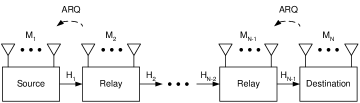
Figure 1: Upper: relay network with direct link from source to destination. Lower: multihop MIMO relay network without direct link.

Assume the packets are delay sensitive: the end-to-end transmission delay cannot exceed $k$. One strategy to achieve this goal is to set a deadline $k_{i}$ for each link $i$ with $\sum_{i=1}^{N-1}k_{i}\leq k$. Once a packet delays more than $k_{i}$ it is removed from the queue. This per-hop delay constraint corresponds to the finite buffer at each node. Another strategy is to allow large per-hop delay while imposing an end-to-end delay constraint. Other assumptions we have made for the channel models are

• The channel between the $i$th and ($i+1$)th nodes is given by:

  $$\boldsymbol{Y}_{i,l}=\sqrt{\frac{SNR}{M_{i}}}\boldsymbol{H}_{i,l}\boldsymbol{X}_{i,l}+\boldsymbol{W}_{i,l},\quad 1\leq l\leq L_{i}.$$ (1)

  The message is encoded by a space-time encoder into a sequence of $L$ matrices $\{\boldsymbol{X}_{i,l}\in\mathcal{C}^{M_{i}\times T},:l=1,\cdots,L\}$, where $T$ is the block length, and $\boldsymbol{Y}_{i,l}\in\mathcal{C}^{M_{i+1}\times T}$, $i=1,\cdots,N-1$, is the received signal at the $(i+1)$th node, in the $l$th ARQ round. The rate of the space-time code is $R$. Channels are assumed to be frequency non-selective, block Rayleigh fading and independent of each other, i.e., the entries of the channel matrices $\boldsymbol{H}_{i,l}\in\mathcal{C}^{M_{i+1}\times M_{i}}$ are independent and identically distributed (i.i.d.) complex Gaussian with zero mean and unit variance. The additive noise terms $\boldsymbol{W}_{i,l}$ are also i.i.d. complex Gaussian with zero mean and unit variance. The forward links and ARQ feedback links only exist between neighboring nodes.

• We consider both the full-duplex and half-duplex relays (see, e.g., [4]) where the relays can or cannot transmit and receive at the same time, respectively, as shown in Fig. 2. Assume the relays use a decode-and-forward protocol (see, e.g., [4]).

• We assume a short-term power constraint at each node for each block code. Hence we do not consider power control.

• We consider both the long-term static channel, where $\boldsymbol{H}_{i,l}=\boldsymbol{H}_{i}$ for all $l$, i.e. the channel state remains constant during all the ARQ rounds, and independent for different $i$. Our results can be extended to the the short-term static channel using the DMDT analysis given in [4].

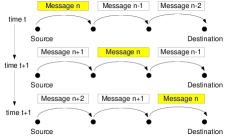
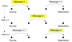
Figure 2: Left: full duplex multihop relay network. Right: half duplex relay multihop MIMO relay network.

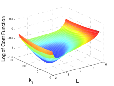
Figure 3: The logarithm of the cost function (10) for the (4, 1, 2) multihop MIMO relay networks. SNR is 20 dB.

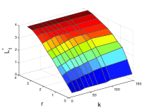
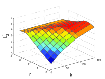
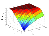
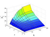
Figure 4: Allocations of optimal ARQ: $L_{1}^{*}$, $L_{2}^{*}$, $L_{1}^{*}+L_{2}^{*}$, $k_{1}^{*}$, in a (4, 1, 2) MIMO relay network. SNR is 20 dB. (The optimal $k_{2}^{*}=k-k_{1}^{*}$.)

II-B Queueing Network Model

We use an $M/M/1$ queue tandem to model the multihop relay networks. The packets arrive at the source as a Poisson process with mean interarrival time $\mu$, (i.e., the time between the arrival of the $n$th packet and $(n-1)$th packet.) The random service time depends on the channel state and is upper bounded by the maximum ARQ rounds allocated $L_{i}$. As an approximation we assume the random service time at Node $i$ for each message is i.i.d. with exponential distribution and mean $L_{i}$. With this assumption we can treat each node as an $M/M/1$ queue. This approximation makes the problem tractable and characterizes the qualitative behavior of MIMO multihop relay network. Node $i$ has a finite buffer size. The packets enter into the buffer and are first-come-first-served (FCFS). Assume $\mu\geq L_{i}$ so that the queues are stable, i.e., the waiting time at a node does not go to infinity as time goes on. Burke’s theorem (see, e.g., [7]) says that the packets depart from the source and arrive at each relay as a Poisson process with rate $p_{i}/\mu$, where $p_{i}$ is the probability that a packet can reach the $i$th node. With high SNR, the packet reaches the subsequent relays with high probability: $p_{i}\approx 1$ (the probability of a packet dropping is small because it uses up the maximum ARQ round.) Hence all nodes have packets arrive as a Poisson process with mean inter-arrival time $\mu$.

II-C Throughput

Denote by $b$ the size of the information messages in bits, $B[t]$ the number of bits removed from transmission buffer at the source at time slot $t$. Define a renewal event as the event that the transmitted message leaves the source and eventually is received by the destination node possibly after one or more ARQ retransmissions. We assume that under full-duplex relays the transmitter cannot send a new message until the previous message has been decoded by the relay at which point the relay can begin transmission over the next hop (Fig. 2a.) Under half duplex relays we assume transmitter cannot send a new message until the relay to the next hop completes its transmission (Fig. 2b.)

The number of bits $\bar{B}$ transmitted in each renewal event, for full-duplexing $\bar{B}=(N-1)b$, and for half-duplexing $\bar{B}=(N-1)b/2$ when $N$ is odd, and $\bar{B}=Nb/2$ when $N$ is even. The long-term average throughput of the ARQ protocol is defined as the transmitted bits per channel use (PCU) [2], which can be found using renewal theory [8]:

$$\eta = \liminf_{s\rightarrow\infty}\frac{1}{Ts}\sum_{t=1}^{s}B[t]=\frac{\bar{B}}{E(\tau)}\doteq\frac{\bar{B}}{(N-1)T}$$ (5)

$$= \left\{\begin{array}[]{ll}R,&\hbox{Full duplex;}\\ \frac{R}{2},&\hbox{Half duplex, $N$ is odd;}\\ R\left(\frac{1}{2}+\frac{1}{2N}\right),&\hbox{Half duplex, $N$ is even.}\\ \end{array}\right.$$

where $\tau$ is the average duration from the time a packet arrives at the source until it reaches the destination node, and $\doteq$ denotes asymptotic equality. A similar argument as in [2] shows that $E(\tau)\doteq(N-1)T$ for high SNR.

II-D Diversity-Multiplexing-Delay Tradeoff

The probability of error $P_{e}$ in the transmission has two sources: from the ARQ error: the packet is dropped because the receiver fails to decode the message within the allocated number of ARQ rounds, denoted as $P_{\mbox{\tiny{ARQ}}}$, and the probability that a message misses its deadline at any node due to large queueing delay, denoted as $P_{\mbox{\tiny{Queue}}}$. We will give $P_{e}$ for various ARQ relay networks. Following the framework of [1], we assume the size of information messages $b(\rho)$ depends on the operating signal-to-noise ratio (SNR) $\rho$, and a family of space time codes $\{\mathcal{C}_{\rho}\}$ with block rate $R(\rho)=b(\rho)/T\triangleq r\log\rho$. We use the effective ARQ multiplexing gain and the ARQ diversity gain [2]

$$r_{e}\triangleq\lim_{\rho\rightarrow\infty}\frac{\eta(\rho)}{\log\rho},\quad d\triangleq-\lim_{\rho\rightarrow\infty}\frac{\log P_{e}(\rho)}{\log\rho}.$$ (6)

We cannot assume infinite SNR because otherwise the queueing delay will be zero, as pointed out in [5]. However we assume high SNR to use the DMDT results in our subsequent analysis.

III Diversity, multiplexing, and delay tradeoff via optimal ARQ round allocation

III-A Full-Duplex Relay in Multihop Relay Network

III-A1 Per-Hop Delay Constraint

The probability of error depends on the ARQ window length allocation $L_{i}$, deadline constraint $k_{i}$, multiplexing rate $r$, and SNR $\rho$. For a given $r$ and $\rho$, we have

$$P_{e}(\{L_{i}\},\{k_{i}\}|\rho,r)=$$

$$P_{\mbox{\tiny{ARQ}}}(\rho,\{L_{i}\})+\sum_{i=1}^{N-1}P_{\mbox{\tiny{Queue}}}(D_{i}>k_{i}).$$ (7)

Here $D_{i}$ denotes the random delay at the $i$th link when the queue is stationary. This $P_{e}$ expression is similar to that given by Equation (33) of [5]. Our goal is to allocate per-hop ARQ round $\{L_{i}\}$ and delay constraint $\{k_{i}\}$ to minimize the probability of error $P_{e}$.

For the long-term static channel, using the DMDT analysis results [4] we have:

$$P_{\mbox{\tiny{ARQ}}}(\rho,\{L_{i}\})=\sum_{i=1}^{N-1}\rho^{-f_{i}\left(\frac{r}{L_{i}}\right)}.$$ (8)

Here $f_{i}(r)$ is the diversity-multiplexing tradeoff (DMT) for a point-to-point MIMO system formed by nodes $i$ and $i+1$. Assuming sufficient long block lengths, $f_{i}(r)$ is given by Theorem 2 in [1] quoted in the following:

Theorem 1

[1] For sufficiently long block lengths, the diversity-multiplexing tradeoff (DMT) $f(r)$ for a MIMO system with $M_{t}$ transmit and $M_{r}$ receive antennas is given by the piece-wise linear function connecting the points $(r,(M_{t}-r)(M_{r}-r)),$ for $r=0,\cdots,\min(M_{t},M_{r})$.

Denote the amount of time spent in the $i$th node by the $n$th message as $D_{n}^{i}$. The probability of packet loss $P_{\mbox{\tiny{Queue}}}(D_{i}>k_{i})$ can be found as the limiting distribution of $\lim_{n\rightarrow\infty}P(D_{n}^{i}>k_{i})$ (adapted from Theorem 7.4.1 of [8]):

Lemma 2

The limiting distribution of the event that the delay at node $i$ exceeds its deadline $k_{i}$, for $M/M/1$ queue models, is given by:

$$P_{\mbox{\tiny{Queue}}}(D_{i}>k_{i})=\lim_{n\rightarrow\infty}P(D_{n}^{i}>k_{i})=\frac{L_{i}}{\mu}e^{-k_{i}\left(\frac{1}{L_{i}}-\frac{1}{\mu}\right)}.$$ (9)

Here the difference in the service rate and packet arrival rate $\frac{1}{L_{i}}-\frac{1}{\mu}\geq 0$ and utility factor $\frac{L_{i}}{\mu}$ both indicate how “busy” node $m$ is. Using the above results, (7) can be written as

$$P_{e}\left(\{L_{i}\},\{k_{i}\}|\rho,r\right)=\sum_{i=1}^{N-1}\left[\rho^{-f_{i}\left(\frac{r}{L_{i}}\right)}+\frac{L_{i}}{\mu}e^{-k_{i}\left(\frac{1}{L_{i}}-\frac{1}{\mu}\right)}\right].$$ (10)

Note that the queueing delay message loss error probability is decreasing in $L_{i}$, and the ARQ error probability is increasing in $L_{i}$. Hence an optimal ARQ rounds allocation at each node $L_{i}$ should trade off these two terms. Also, the optimal ARQ allocation should also equalize the performance of each link, as the weakest link determines the system performance[4].

Hence the optimal ARQ allocation can be formulated as the following optimization problem:

$$\begin{split}\min_{\{L_{i}\},\{k_{i}\}\in\mathcal{A}}&P_{e}(\{L_{i}\},\{k_{i}\}|\rho,r)\end{split}$$ (11)

where

$$\mathcal{A}=\left\{\begin{array}[]{l}\sum_{i=1}^{N-1}L_{i}\leq L,\\ 1\leq L_{i}\leq\mu,\quad i=1,\cdots,N-1\\ \sum_{i=1}^{N-1}k_{i}\leq k.\\ \end{array}\right\}$$ (15)

The following lemma (proof omitted due to the space limit) shows that the total transmission distortion function (21) is convex in the interior of $\mathcal{A}$.

Lemma 3

The transmission distortion function (21) is convex jointly in $L_{i}$ and $k_{i}$ in the convex set

$$\left\{\{L_{i}\},\{k_{i}\}:k_{i}>\frac{L_{i}}{2(\frac{\mu}{L_{i}}-1)},\quad i=1,\cdots N-1.\right\},$$

Lemma 3 says that except for the “corners” of $\mathcal{A}$ the cost function is convex. However these “corners” have higher probability of error: $k_{i}$ and $L_{i}$ take extreme values and hence one link may have a longer queueing delay then the others. So we only need to search the interior of $\mathcal{A}$ where the cost function is convex.

To gain some insights into where the optimal solution resides in the feasible domain for the above problem, we present a marginal cost interpretation. Note that the probability of error can be decomposed as a sum of probability of error on the $i$th link. The optimal ARQ rounds allocated on this link should equalize the “marginal cost” of the ARQ error and the packet loss due to queueing delay. For node $i$, with fixed $k_{i}$, the marginal costs (partial differentials) of the ARQ error probability, and the packet loss probability due to queueing delay, with respect to $L_{i}$ are given by

$$\frac{\partial\rho^{-f_{i}\left(\frac{r}{L_{i}}\right)}}{\partial L_{i}}=\frac{r}{L_{i}^{2}}f^{\prime}_{i}\left(\frac{r}{L_{i}}\right)\rho^{-f_{i}\left(\frac{r}{L_{i}}\right)}\ln\rho<0,$$ (16)

and

$$\frac{\partial P_{\mbox{\tiny{Queue}}}(D_{i}>k_{i})}{\partial L_{i}}=\frac{1}{\mu}\left(1+\frac{k}{L_{i}}\right)e^{-k_{i}\left(\frac{1}{L_{i}}-\frac{1}{\mu}\right)}>0.$$ (17)

Note that $f^{\prime}_{i}<0$. The optimal solution equalizes these two marginal costs by choosing $L_{i}\in[1,\mu]$. Note that these marginal cost functions are monotone in $L_{i}$, hence the equalizing $L_{i}^{*}$ exists and $1<L_{i}^{*}<\mu$ if the following two conditions are true for $L_{i}=1$ and $L_{i}=\mu$:

$$(i):\left.\frac{\partial P_{\mbox{\tiny{Queue}}}(D_{i}>k_{i})}{\partial L_{i}}\right|_{L=1}<-\left.\frac{\partial\rho^{-f_{i}\left(\frac{r}{L_{i}}\right)}}{\partial L_{i}}\right|_{L=1},$$ (18)

$$(ii):\left.\frac{\partial P_{\mbox{\tiny{Queue}}}(D_{i}>k_{i})}{\partial L_{i}}\right|_{L=\mu}>-\left.\frac{\partial\rho^{-f_{i}\left(\frac{r}{L_{i}}\right)}}{\partial L_{i}}\right|_{L=\mu},$$ (19)

These conditions involve nonlinear inequalities involving $\mu$, $\rho$, $r$, $M_{i}$ and $M_{i+1}$, which defines the case when the optimal solution is in the interior of $\mathcal{A}$. Analyzing these conditions reveals that these conditions tend to satisfy at lower multiplexing gain $r$, small $M_{i}$ or $M_{i+1}$, small $k_{i}$, and larger $\mu$ (light traffic). Note that with high SNR condition (ii) is always true for moderate $k$ values. When $(i)$ and $(ii)$ are violated, which means one error dominates the other, then the optimal solution lies at the boundary of $\mathcal{A}$. With the total ARQ rounds constraint in (11), using the Lagrangian multiplier an argument similar to above still holds.

III-A2 End-to-End Delay constraint

When the buffer per node is large enough a per hop delay constraint is not needed, and we can instead impose an end-to-end delay constraint. The exact expression for the tail probability of the end-to-end delay is intractable. However a large deviation result is available. The following theorem can be derived using the main theorem in [9]:

Theorem 4

For a stationary $M/M/1$ queue tandem (with full-duplex relays):

$$\lim_{k\rightarrow\infty}\lim_{n\rightarrow\infty}\frac{1}{k}\log P_{\mbox{\tiny{Queue}}}\left(\sum_{i=1}^{N-1}D_{n}^{i}\geq k\right)=-\theta^{*},$$

where $\theta^{*}=\min_{i=1}^{N-1}\left\{\frac{1}{L_{i}}-\frac{1}{\mu}\right\}$.

This theorem says that the bottleneck of the queueing network is the link with longest mean service time $L_{i}$. Hence the optimal ARQ round allocation problem can be formulated as:

$$\min_{\{L_{i}\}\in\mathcal{B}} P_{e}(\{L_{i}\},\{k_{i}\}|\rho,r)$$ (20)

where

$$P_{e}\left(\{L_{i}\},\{k_{i}\}|\rho,r\right)$$

$$=P_{\mbox{\tiny{ARQ}}}(\rho,\{L_{i}\})+P_{\mbox{\tiny{Queue}}}\left(\sum_{i=1}^{N-1}D_{n}^{i}\geq k\right),$$

$$\doteq\sum_{i=1}^{N-1}\rho^{-f_{i}\left(\frac{r}{L_{i}}\right)}+e^{-\theta^{*}k}.$$ (21)

$$\mathcal{B}=\left\{\begin{array}[]{l}\sum_{i=1}^{N-1}L_{i}\leq L,\\ 1\leq L_{i}\leq\mu,\quad i=1,\cdots,N-1\end{array}\right\}$$ (24)

For high SNR, this can be shown to be a convex optimization problem. A simple argument can show that the packet loss probability with the per-hop delay constraint is larger than that using the more flexible end-to-end constraint.

III-B Half-duplex Relay in Multihop Network

Half-duplex relay is not a standard queue tandem model. However we can also derive a large deviation result for the tail probability for the end-to-end delay of a multihop network with half-duplex relays (proof in the Appendix):

Theorem 5

For a stationary $M/M/1$ queue tandem (with half-duplex relays), when the number of node $N$ is large:

$$\lim_{k\rightarrow\infty}\lim_{n\rightarrow\infty}\frac{1}{k}\log P_{\mbox{\tiny{Queue}}}\left(\sum_{i=1}^{N-2}D_{n}^{i}\geq k\right)=-\theta^{*}.$$ (25)

From this theorem we conclude that the optimal ARQ allocation problem with the end-to-end constraint and half-duplex relays can be formulated the same as that with full-duplex relays (20).

IV Numerical Examples

Consider a MIMO relay network consists of a source, a relay, and a destination node. The relay is full-duplex. The number of antennas on each node is $(M_{1},M_{2},M_{3})$, $M_{1}=4$, $M_{2}=1$, and $M_{3}=2$, where the relay has a single antenna. Other parameters are: $\rho=20$dB, $k=30$, $L=8$, and the multiplexing gain is $r=2$. The base 10 logarithm of the cost function (10) is shown in Fig. 3. We have optimized the cost function with respect to $L_{2}$ and $k_{2}$ so we can display it in three dimensions. Note that the surface is convex in the interior of the feasible region. The optimal $L_{1}^{*}$, $L_{2}^{*}$, $k_{1}^{*}$ are shown in Fig. 4. Also note that as $r$ increases to the maximum possible $r=4$, the total number of ARQ rounds allocated $L_{1}^{*}+L_{2}^{*}$ gradually increases to the upper bound $L=8$ as $k$ increases.

V Conclusions and Future Work

We have studied the diversity-multiplexing-delay tradeoff in multihop MIMO networks by considering an optimal ARQ allocation problem to minimize the probability of error, which consists of the ARQ error and the packet loss due to queueing delay. Our contribution is two-fold: we combine the DMDT analysis with queueing network theory, and we use the tail probability of random delay to find the probability of packet loss due to queueing delay. Numerical results show that optimal ARQ should equalize the performance of each link and avoid long service times that cause large queueing delay. Future work will investigate joint source-channel coding in multihop MIMO relay networks, extending the results of [5].

Proof of Theorem 5

For node $i$, $i=1\cdots N$, let the random variable $S_{n}^{i}$ denotes the service time required by the $n$th customer at the $i$th node (the number of ARQs used for the $n$th packet), and $A_{n}^{i}$ be the inter arrival time of the $n$th packets (i.e., the time between the arrival of the $n$th and $(n-1)$th packages to this node). The waiting time of the $n$th packet at the $i$th node $W_{n}^{i}$ satisfies Lindley’s recursion (see [9]):

$$W_{n}^{i}=(W_{n-1}^{i}+S_{n-1}^{i+1}-A_{n}^{i})^{+},\quad 2\leq i\leq N-2,$$ (26)

where $(x)^{+}=\max(x,0)$. The total time a message spent in a node is its waiting time plus its own service time, hence

$$D_{n}^{i}=W_{n}^{i}+S_{n}^{i}.$$ (27)

The arrival process to the $(i+1)$th node is the departure process from the $i$th node, which satisfies the recursion:

$$A_{n}^{i}=A_{n}^{i-1}+D_{n}^{i-1}-D_{n-1}^{i},\quad 2\leq i\leq N-2.$$ (28)

with $A_{n}^{i}$ a Poisson process with rate $1/\mu$. Also the waiting time at the source satisfies:

$$W_{n}^{1}=(W_{n-1}^{1}+S_{n-1}^{1}+S_{n-1}^{2}-A_{n}^{1})^{+}.$$ (29)

A well-known result is that (see, e.g. [9]), if the arrival and service processes satisfy the stability condition, then the Lindley’s recursion has the solution:

$$W_{n}^{i} = \max_{j_{i}\leq n}(\sigma^{i}_{j_{i},n-1}-\tau^{i}_{j_{i}+1,n}),\quad i=2,\cdots N-2,$$

$$W_{n}^{1} = \max_{j_{1}\leq j_{2}}(\sigma^{1}_{j_{1},j_{2}-1}+\sigma^{2}_{j_{1},j_{2}-1}-\tau^{1}_{j_{1}+1,j_{2}}).$$ (30)

where the partial sum $\tau_{l,p}^{i}=\sum_{k=l}^{p}A_{k}^{i}$ and $\sigma_{l,p}=\sum_{k=l}^{p}S_{k}^{i}$. Hence

$$D_{n}^{i}=\max_{j_{i}\leq n}(\sigma^{i}_{j_{i},n-1}+S_{n}^{i}-\tau^{i}_{j_{i}+1,n}),\quad i=2,\cdots N-2.$$ (31)

From (28) we have $\tau_{l,p}^{i}=\tau_{l,p}^{i-1}+D_{p}^{i-1}-D_{l-1}^{i-1}$ for $l\leq p+1$, and 0 otherwise. Plug this into (31) we have

$$D_{n}^{i}=\max_{j_{i}\leq n}(\sigma^{i+1}_{j_{i},n-1}+S_{n}^{i}-\tau_{j_{i}+1,n}^{i-1}-D_{n}^{i-1}+D_{j_{i}}^{i-1}).$$ (32)

Hence the recursive relation if we move $D_{n}^{i-1}$ to the left-hand-side:

$$D_{n}^{i}+D_{n}^{i-1}=\max_{j_{i}\leq n}(\sigma_{j_{i},n-1}^{i+1}+S_{n}^{i}-\tau_{j_{i}+1,n}^{i-1}+D_{j_{i}}^{i-1}).$$ (33)

Now from (31) we have $D_{j_{i}}^{i-1}=\max_{j_{i-1}\leq j_{i}}(\sigma^{i}_{j_{(i-1)},j_{i}-1}+S_{j_{i}}^{i-1}-\tau_{j_{(m-1)}+1,j_{m}}^{i-1})$. Plug this in the above (33) we have

$$D_{n}^{i}+D_{n}^{i-1}$$

$$= \max_{j_{(i-1)}\leq j_{i}\leq n}(\sigma_{j_{i},n-1}^{i+1}+S_{n}^{i}+\sigma^{i}_{j_{(i-1)},j_{i}-1}+S_{j_{i}}^{i-1}-\tau_{j_{(i-1)}+1,n}^{i-1})$$

Do this inductively, we have

$$\sum_{i=2}^{N-2}D_{n}^{i}=\max_{j_{2}\leq\cdots\leq j_{N-1}=n}\left[\sum_{m=2}^{N-2}(\sigma^{i+1}_{j_{i},j_{(i+1)}-1}+S_{j_{i+1}}^{i})-\tau^{1}_{j_{2}+1,n}\right].$$

If we also add $D_{n}^{1}=W_{n}^{1}+S_{n}^{1}$ to the above equation, after rearranging terms we have:

$$\sum_{i=1}^{N-2}D_{n}^{i}=\sum_{i=2}^{N-2}(\sigma^{i}_{j_{(i-1)},j_{i}-1}+S_{j_{(i+1)}}^{i})-\tau^{1}_{j_{2}+1,n}$$

$$+S_{j_{2}}^{1}+\sigma_{j_{1},j_{2}-1}^{1}+S_{j_{2}}^{2}+\sigma_{j_{N-2},j_{(N-1)}-1}^{N-1}.$$ (34)

Note that $\sigma^{i}_{j_{(i-1)},j_{i}-1}$ is independent of $S_{j_{(i+1)}}^{i}$. For long queue we can ignored the last four terms caused by edge effect (the source and end queue of the multihop relay network). By stationarity of the service process $\sigma^{i}_{j_{(i-1)},j_{i}-1}+S_{j_{(i+1)}}^{i}$ has the same distribution as $\sigma^{i}_{0,j_{i}-j_{(i-1)}}$. Then (34) reduces to the case studied in [9] and we can borrow the large deviation argument therein to derive the exponent $\theta^{*}$.

References

- [1] L. Zheng and D. N. C. Tse, “Diversity and multiplexing: A fundamental tradeoff in multiple-antenna channels,” IEEE Trans. Inform. Theory, vol. 49, pp. 1073–1096, 2003.
- [2] H. El Gamal, G. Caire, and M. O. Damen, “The MIMO ARQ channel: Diversity-multiplexing-delay tradeoff,” IEEE Trans. Inform. Theory, vol. 52, pp. 3601–3621, 2006.
- [3] T. Tabet, S. Dusad, and R. Knopp, “Diversity-multiplexing-delay tradeoff in half-duplex ARQ relay channels,” IEEE Transactions on Information Theory, vol. 53, pp. 3797–3805, October 2007.
- [4] Y. Xie, D. Gunduz, and A. Goldsmith, “Multihop MIMO relay networks with ARQ,” IEEE Globecom 2009 Communication Theory Symposium, Dec. 2009.
- [5] T. Holliday, A. J. Goldsmith, and H. V. Poor, “Joint source and channel coding for MIMO systems: Is it better to be robust or quick?,” IEEE Transactions on Information Theory, vol. 54, no. 4, 2008.
- [6] N. Bisnik and A. Abouzeid, “Queueing network models for delay analysis of multihop wireless Ad Hoc networks,” pp. 773 – 778, Proceedings of the 2006 International Conference on Wireless Communications and Mobile Computing, July 2006.
- [7] G. Bolch, S. Greiner, and H. de Meer, Queueing Networks and Markov Chains : Modeling and Performance Evaluation With Computer Science Applications. Springer Series in Statistics, Wiley-Interscience, 2 ed., Aug. 2006.
- [8] S. M. Ross, Stochastic Processes. John Wiley & Sons, 2 ed., 1995.
- [9] A. J. Ganesh, “Large deviations of the sojourn time for queues in series,” Annals of Operations Research, vol. 79, pp. 3–26, Jan. 1998.