Collective modes as a probe of imbalanced Fermi gases

Abstract

We theoretically investigate the collective modes of imbalanced two component one-dimensional Fermi gases with attractive interactions. This is done for trapped and untrapped systems both at zero and non-zero temperature, using self-consistent mean-field theory and the random phase approximation. We discuss how the Fulde-Ferrell-Larkin-Ovchinnikov (FFLO) state can be detected and the periodicity of the associated density modulations determined from its collective mode spectrum. We also investigate the accuracy of the single mode approximation for low-lying collective excitations in a trap by comparing frequencies obtained via sum rules with frequencies obtained from direct collective mode calculations. It is found that, for collective excitations where the atomic clouds of the two spin species oscillate largely in phase, the single mode approximation holds well for a large parameter regime. Finally we investigate the collective mode spectrum obtained by parametric modulation of the coupling constant.

I Introduction

With the advancements in the field of ultracold atomic gases new phases of matter are becoming experimentally accessible. Superfluidity bloch07 ; pitaevskii_stringari_RMP_09 and density imbalance pairing_and_phase_sep_in_pol_fg_partridge_hulet ; fermionic_sf_with_imbalanced_populations-zwierlein-ketterle06 in two component Fermi gases have been demonstrated experimentally. Together these offer the exciting perspective of achieving the Fulde-Ferrell-Larkin-Ovchinnikov (FFLO) phase larkin_ovchinnikov_64 ; superconductivity_in_spin_exch_field_fulde_ferrell64 , an unconventional superfluid state in imbalanced Fermion systems. It has been under theoretical investigation since the 1960s but has so far eluded unambiguous experimental detection.

In solid state systems the detection of the FFLO phase is unfavourable since density imbalances between spin up and down electrons need to be imposed via Zeeman splitting, requiring strong magnetic fields. This in turn destroys superconductivity via diamagnetic effects landau_lifshitz_pitaevskii_stat_phys_part2 . Ultracold atomic gases are favourable for its detection since it is possible to set the density imbalance of the system simply by adjusting the number of spin up and down particles which are loaded into the atomic trap pairing_and_phase_sep_in_pol_fg_partridge_hulet ; fermionic_sf_with_imbalanced_populations-zwierlein-ketterle06 .

Theory does predict the occurrence of the FFLO phase in three-dimensional (3D) ultracold Fermi gases though the region of parameter space it occupies is thought to be relatively small (for a review see bec-bcs_xover_in_pol_res_SF-radzihovsky ). On the other hand the FFLO phase is expected to be stabilised in quasi one-dimensional (1D) geometries which can be imposed using optical lattices bloch07 ; orso_attr_fermi_gases_bethe_ansatz07 ; phase_diag_of_str_int_pol_fg_1d_drummond07 ; pairing_states_of_pol_fg_feiguin_meisner07 ; quasi_1d_pol_fermi_SFs-parish-huse07 ; batrouni_scalettar_09 ; fflo_state_in_1d_attr_hubbard_model_luescher_laeuchli08 .

In a recent development one-dimensional imbalanced Fermi gas systems have been created in experiment spin_imbalance_in_a_1d_FG-Liao_Hulet_2009 . These recent experimental results indicate that the density distribution is of the form expected for the partially-polarised state associated with the FFLO phase. However, a direct demonstration of the ordering in the FFLO phase remains to be shown. An important question which now arises, is how best to detect this characteristic ordering of the FFLO phase. Previous proposals for the detection of the FFLO phase include detecting characteristic peaks in the expansion image following release of the trap bec-bcs_xover_in_pol_res_SF-radzihovsky , the probing of noise correlations in an expansion image fflo_state_in_1d_attr_hubbard_model_luescher_laeuchli08 , and the use of RF spectroscopy to excite atoms out of the gas into other states spectral_signatures_of_fflo_in_1d_bakhtiari_torma . In a recent letter signature_of_fflo_first_paper_jonathan_nigel we showed how the FFLO phase in 1D at $T=0$ can be detected via its collective mode signature. In this paper we extend this discussion to non-zero temperature and discuss other aspects of collective modes in imbalanced Fermi gases. Collective modes have proved very useful for probing the properties of ultracold balanced pitaevskii_stringari_RMP_09 and imbalanced normal_state_of_a_polarized_FG_at_unit_Lobo06 ; collective_osc_of_imb_FG_polaron_nascimbene_salomon ; coll_ex_of_trapped_imb_FG-schaeybroeck08 ; trapped_2d_FG_with_pop_imbalance-schaeybroeck09 Fermi gases. Our work extends these discussions to one dimension and the presence of the FFLO state.

The paper is organised as follows. In Sec. II we present the theoretical model of our study. In Sec. III we describe the homogeneous system and present our results for the associated collective mode spectrum. We describe the speed of sound as a function of the polarisation of the Fermi gas and highlight the collective mode signature of the FFLO phase. We then discuss the effects of nonzero temperature. In Sec. IV we turn our attention to the trapped Fermi gas. We assess the accuracy of the single mode approximation for various low-frequency modes in a trap. We then investigate the effect of the FFLO phase on the collective mode spectrum of the trapped imbalanced Fermi gas. From this we deduce a signature of the presence of the FFLO phase in the collective mode spectrum. Finally we describe the response of the trapped Fermi gas to a modulation of the coupling constant.

II Theoretical model

We study a model of a two-component Fermi gas in one dimension with attractive contact interactions and unequal densities. For a homogeneous system, the exact groundstates orso_attr_fermi_gases_bethe_ansatz07 ; phase_diag_of_str_int_pol_fg_1d_drummond07 ; Phase_trans_pairing_sig_attractive_Fermi_gases-guan07 ; exact_anal_of_delta_fn_spin_half_attr_FG-Iida08 ; magnetism_and_quantum_phase_trans-he_batchelor09 and thermodynamics anal_thermodyn_and_thermometr_of_gaudin_yang_gases-zhao_oshikawa09 are known from the Bethe ansatz some_exact_results_for_many_body_problem_in_1d_w_delta_int-yang_prl67 ; un_systeme_a_une_dimension_de_fermions_en_interaction-gaudin67 ; thermodyn_of_1d_solvable_models-takahashi . As has been discussed in detail by Liu et al. liu_drummond_07 , Bogoliubov de Gennes (BdG) mean-field theory provides an accurate description of the exact phase diagram for the 1D system, at least within the weak-coupling BCS regime. We have extended the mean-field theory to investigate the linear response and collective modes of both the trapped and untrapped imbalanced Fermi gas.

Our numerical calculations are based on the discretised Bogoliubov de Gennes Hamiltonian which is given by

$$\hat{H} = -J\sum_{i,\sigma}\left(\hat{c}^{\dagger}_{i+1,\sigma}\hat{c}_{i,\sigma}+h.c.\right)$$ (1)

$$+\sum_{i}\left(\Delta_{i}\hat{c}^{\dagger}_{i,\uparrow}\hat{c}^{\dagger}_{i,\downarrow}+h.c.\right)+\sum_{i,\sigma}W_{i,\sigma}\hat{c}^{\dagger}_{i,\sigma}\hat{c}_{i,\sigma}$$

where $\hat{c}_{i,\sigma}^{(\dagger)}$ are fermionic operators for species $\sigma=\uparrow,\downarrow$ on site $i$, $W_{i,\sigma}\equiv V^{ext}_{i}+V^{int}_{i,\sigma}-\mu_{\sigma}$ (with $V^{ext}$ the external potential, $V^{int}_{i,\sigma}=U\langle\hat{c}^{\dagger}_{i,\bar{\sigma}}\hat{c}_{i,\bar{\sigma}}\rangle$, $\mu_{\sigma}$ the chemical potentials and $\bar{\sigma}$ is the spin opposite to spin $\sigma$) and $\Delta_{i}\equiv U\left\langle\hat{c}_{i,\downarrow}\hat{c}_{i,\uparrow}\right\rangle$ is the local superfluid gap. $J$ is the hopping parameter and $U$ the on-site interaction strength ($U<0$ is assumed throughout). The angled brackets $\left\langle\dots\right\rangle$ denote the thermal and quantum expectation value at temperature $T$. The corresponding Bogoliubov de Gennes equations are solved self consistently to yield the mean field ground state.

The results we present are at sufficiently low particle density to be representative of the continuum limit. In the mapping to the continuum, we relate site $i$ to position $x$ via $x=ia$, the mass is $m=\frac{\hbar^{2}}{2Ja^{2}}$ and the 1D interaction parameter is $g_{1d}=Ua$. The interaction strength $\gamma$, defined as the ratio of the interaction energy density to the kinetic energy density, is given by

$$\gamma=-\frac{mg_{1d}}{\hbar^{2}\rho}$$ (2)

liu_drummond_07 where $\rho$ is the total density of particles. In the case of a trapped system we take $\gamma$ to be defined by the density at the centre of the trap. We restrict our study to values of $\gamma$ up to about $\gamma=1.6$ where mean-field theory gives qualitatively accurate results liu_drummond_07 . The Fermi wavevector for spin $\sigma$ is given by $k_{F\sigma}=\pi\rho_{\sigma}$ where $\rho_{\sigma}$ is the density for spin $\sigma$. We define the polarisation $p$ of the 1D Fermi gas as

$$p \equiv\frac{k_{F,\uparrow}-k_{F,\downarrow}}{k_{F,\uparrow}+k_{F,\downarrow}}\,.$$ (3)

Additionally, we shall find it useful to define $k_{B}T_{F}=E_{F}\equiv\pi^{2}\rho^{2}J/4$. In the remainder of this paper we set $\hbar=1$.

The collective mode spectrum is obtained by considering the linear response of a system to external perturbations. Divergences in the response appear at the frequencies of the collective modes. We obtain the linear response of the equilibrium system by supplementing the Bogoliubov de Gennes equations with a self consistent random phase approximation (RPA). As was pointed out in signature_of_fflo_first_paper_jonathan_nigel and as we will argue in Sec. III.3, this approximate theory correctly captures all qualitative features of the collective modes that are important for our purposes.

The self consistent linear response within RPA is computed as follows. Let

$$\hat{A}_{i}(t) =\left(\hat{\rho}_{i,\uparrow}(t),\hat{\kappa}^{\dagger}_{i}(t),\hat{\kappa}_{i}(r),\hat{\rho}_{i,\downarrow}(t)\right)$$ (4)

where $\hat{\rho}_{i,\sigma}=\hat{c}^{\dagger}_{i,\sigma}(t)\hat{c}_{i,\sigma}(t)$, $\hat{\kappa}^{\dagger}_{i}(t)=\hat{c}^{\dagger}_{i,\uparrow}(t)\hat{c}^{\dagger}_{i,\downarrow}(t)$ in the Heisenberg representation. Furthermore, let $\hat{A}_{i,\alpha}(t)$ ($\alpha\in\{1..4\}$) refer to the four components of $\hat{A}_{i}(t)$ and denote the Fourier transforms of $\hat{A}_{i,\alpha}(t)$ as $\hat{A}_{i,\alpha}(\omega)$. The bare response or single particle response of $\hat{A}_{i,\alpha}$ to a perturbation $\delta\hat{H}(\omega)=\sum_{j,\beta}\delta h_{j,\beta}(\omega)\hat{A}_{j,\beta}(\omega)$ is given by

$$\left\langle\delta\hat{A}_{i,\alpha}(\omega)\right\rangle =\sum_{j,\beta}\chi^{0}_{i\alpha,j\beta}(\omega)\delta h_{j,\beta}(\omega)$$ (5)

where the bare response function $\chi^{0}$ is given by bruun_mottelson01

$$\chi^{0}_{i\alpha,j\beta}(\omega) =\frac{1}{\mathrm{i}}\int_{-\infty}^{\infty}\,\mathrm{d}t\int_{-\infty}^{t}\,\mathrm{d}\tau\left\langle\left[\hat{A}_{i\alpha}(t),\hat{A}_{j\beta}(\tau)\right]\right\rangle\mathrm{e}^{\mathrm{i}\omega t}$$ (6)

The thermal average $\left\langle\dots\right\rangle$ is computed by transforming to the quasiparticle eigenbasis in which $\left\langle\alpha^{\dagger}_{\mu}\alpha_{\nu}\right\rangle=\delta_{\mu,\nu}f(E_{\mu})$ where $\alpha^{\dagger}_{\mu}$ is the quasiparticle creation operator for a quasiparticle with energy $E_{\mu}$ and $f$ is the Fermi function. The self consistent response function $\chi$ is obtained within RPA by taking into account the change in the Hamiltonian due to a change in the quantities $\left\langle\hat{A}_{i,\alpha}\right\rangle$. The perturbing potential will then consist of the external perturbation plus the potential arising from the interaction,

$$\delta\hat{H} =\sum_{j,\beta}\left(\delta h^{\text{ext}}_{j,\beta}\hat{A}_{j,\beta}(\omega)+\sum_{k,\gamma}H^{\text{int}}_{j\beta,k\gamma}\hat{A}_{j,\beta}\left\langle\delta\hat{A}_{k,\gamma}\right\rangle\right)$$ (7)

where bruun_mottelson01

$$H^{\text{int}}_{l\delta,k\gamma} =U\delta_{l,k}K_{\delta,\gamma} \text{and}\qquad K_{\delta,\gamma} =\begin{pmatrix}0&0&0&1\\ 0&0&1&0\\ 0&1&0&0\\ 1&0&0&0\end{pmatrix}\,.$$ (8)

Inserting this into the bare response we obtain:

$$\left\langle\delta\hat{A}_{k,\gamma}(\omega)\right\rangle =\left(\delta_{i,k}\delta_{\alpha,\gamma}-\chi^{0}_{i\alpha,l\delta}H^{\text{int}}_{l\delta,k\gamma}\right)^{-1}\chi^{0}_{i\alpha,j\beta}\delta h^{\text{ext}}_{j,\beta}$$ (9)

(summation implied), which determines the RPA result for the susceptibility.

III Homogeneous system

The ground state of a homogeneous Fermi gas with contact interactions can be found exactly by the Bethe ansatz orso_attr_fermi_gases_bethe_ansatz07 ; phase_diag_of_str_int_pol_fg_1d_drummond07 . For attractive interactions the phase diagram spanned by the two chemical potentials at $T=0$ contains a fully paired region, a fully polarised (and therefore non-interacting) region and a partially polarised region. The latter is associated with the FFLO phase. The mean field ground state was shown to be in good qualitative agreement with the exact ground state liu_drummond_07 . The FFLO phase is characterised by an oscillating order parameter with a wavelength $\lambda_{\Delta}$ and different average densities $\rho_{\sigma}$ for the $\uparrow$ and $\downarrow$ particles. As the pairing suppresses density differences, the density difference $\rho_{\uparrow}(x)-\rho_{\downarrow}(x)$ is maximal at the nodes of the order parameter and minimal at the anti-nodes. For low polarisations it is possible to describe the system as a fully paired superfluid on top of which there is a gas of excess majority spin particles. These are situated at the nodes of the order parameter Yang_inhomogeneous_sc_state_1d_01 ; mizushima07 . At zero temperature the wavevector $k_{\Delta}=\frac{2\pi}{\lambda_{\Delta}}$ for the order parameter is given by $k_{\Delta}=k_{F,\uparrow}-k_{F\downarrow}$. A possible ground state configuration where these quantities are illustrated is shown in Fig. 1. With increasing temperature the order parameter disappears. For interaction strengths we are considering, the FFLO phase disappears at temperatures $T$ on the order of $T/T_{F}=0.1$ finite_temp_phase_diag_of_spin_pol_fg-liu_drummond08 .

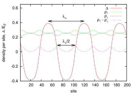
Figure 1: (Colour online) Example of a homogeneous system displaying an FFLO phase. The periodicity of the densities is given by $\lambda_{\Delta}/2$ where $\lambda_{\Delta}$ is the wavelength of the order parameter. This configuration has $\gamma=1.6$ and the polarisation $p=0.06$.

III.1 Sound velocities in an imbalanced gas

We have investigated the speed of sound in a homogeneous system and how it depends on polarisation. For this we compute the response of the system to potentials of the form

$$\delta W_{\sigma}(x,t)=V_{\sigma}\sin kx\cos\omega t\,.$$ (10)

We refer to the case $V_{\uparrow}=V_{\downarrow}=V_{0}$ as a “spin-symmetric” and $V_{\uparrow}=-V_{\downarrow}=V_{0}$ as a “spin-asymmetric” excitation. Eq. (10) represents a standing wave perturbation with a fixed phase. It is sufficient to consider this type of perturbation since we find that changing the phase of the perturbation with respect to the phase of the order parameter does not change our results in any significant way. Throughout this paper we define the response $R$ as

$$R =\sqrt{\sum_{i}\left(\delta\rho_{i,\uparrow}^{2}+\delta\rho_{i,\downarrow}^{2}\right)}$$ (11)

which is a measure of the change in the density.

For nonzero polarisations when the FFLO state is present two distinct sound modes exist with in general different velocities, as shown in Fig. 2. This can be understood within mean field theory from the fact that the FFLO phase breaks both gauge and translational symmetry. However, as we will argue in Sec. III.3, these results are fully consistent with those expected from exact theory.

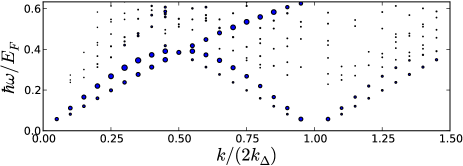
Figure 2: (Colour online) Response of a homogeneous system in the FFLO phase to a spin-asymmetric periodic potential (10). The area of the circle is proportional to the amplitude of the response. The polarisation is $p=0.15$, and the interactions strength is $\gamma=1.5$. Two gapless sound modes are seen to emerge around $k\simeq 0$ and $k\simeq k^{*}\equiv 2k_{\Delta}$. The simulation was done on 270 lattice sites. The divergent response at $\omega=0$ is not shown.

The sound velocities at $T=0$ of these two modes as a function of the polarisation are shown in Fig. 3. (Small fluctuations in the lattice filling due to the technique used lead to small variations in the sound velocity sound_velocity_and_dim_crossover_in_sf_FG-koponen-Torma .) For very low polarisations we effectively have a paired superfluid on top of which there is a weakly interacting gas of excess majority spin particles, which are located at the positions of the domain walls in the order parameter Yang_inhomogeneous_sc_state_1d_01 ; mizushima07 . In this regime of low polarisation one of the sound modes is associated with phase fluctuations of the order parameter, and has a very similar velocity as that for a spin balanced superfluid. The other sound mode, with lower velocity, arises from the motions of the excess majority spin particles (the domain walls). The speed of sound of this mode becomes very small (below the resolution of our calculation) at very low polarisations, as the domain walls become very dilute and cease to overlap.

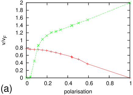
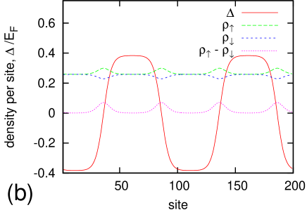
Figure 3: (Colour online) (a) Sound velocity versus polarisation for interaction strength $\gamma\approx 1.6$. $v_{F}=\frac{1}{2}(v_{F,\uparrow}+v_{F,\downarrow})$. As $p\to 0$ the velocity of one of the sound modes disappears. As soon as the domain walls between regions of positive $\Delta$ and negative $\Delta$ cease to overlap the sound velocity drops below our numerical resolution. This is because shifting the position of a domain wall costs very little energy. (b) Order parameter and density distributions for a polarisation ($p=0.038$) at which the domain walls cease to overlap.

In the other limit, $p\to 1$, one of the sound modes vanishes, whereas the higher velocity mode tends to the value for a non-interacting Fermi gas.

III.2 Signature of the FFLO phase

We now turn to the signature of the FFLO phase in the collective mode spectrum. Again we investigate the response of the system to potentials of the form (10). However, this time we concentrate on short wavelength perturbations.

For zero temperature there is a clear signature of the FFLO phase in the response spectrum of a homogeneous Fermi gas. As illustrated in Fig. 2 this manifests itself in sound modes emerging around $k=k^{*}=2k_{\Delta}$ in addition to the ones emerging around $k=0$ signature_of_fflo_first_paper_jonathan_nigel . Within mean-field theory, this can be understood as a consequence of the broken translational symmetry of the FFLO phase, though this too is fully consistent with exact theory (see Sec. III.3).

These low energy sound modes are due to a Brillouin zone (BZ) arising from the spatial periodicity of the superfluid order parameter $\Delta(x)$. The consequence is a generalised Bloch theorem. Let $\hat{T}$ be the operator which performs the transformation: $x\to x+\lambda_{\Delta}/2,\;\Delta(x)\to-\Delta(x)$. For a system with an FFLO wavelength of $\lambda_{\Delta}$, $\hat{T}$ commutes with the Hamiltonian (1) since $\rho_{\uparrow}$ and $\rho_{\downarrow}$ have periodicities $\lambda_{\Delta}/2$. Note that $\hat{T}$ encodes the smallest translational shift for which such a symmetry exists. As the Hamiltonian commutes with $\hat{T}$, the density matrix $\hat{\rho}_{0}$ for the equilibrium configuration is invariant under $\hat{T}^{-1}\hat{\rho}_{0}\hat{T}$ and $\hat{T}$ is time-independent. In the continuum limit the response of the system is given by

$$\left\langle\delta\hat{A}_{\alpha}(r,t)\right\rangle =\sum_{\beta}\int_{-\infty}^{t}\,\mathrm{d}\tau\int\,\mathrm{d}r^{\prime}\;\chi^{0}_{\alpha,\beta}(r,r^{\prime},t,\tau)\;\delta h_{\beta}(r^{\prime},\tau).$$ (12)

Within linear response $\chi^{0}$ is given by forster75

$$\chi^{0}_{\alpha,\beta}(r,r^{\prime},t,\tau) =\frac{1}{\mathrm{i}}\left\langle\left[\hat{A}_{\alpha}(r,t),\hat{A}_{\beta}(r^{\prime},\tau)\right]\right\rangle.$$ (13)

As described above, in the self consistent random phase approximation $\delta\hat{H}$ is given by an externally applied perturbation plus a self consistent perturbation. Consider free oscillations, i.e. the external perturbation is set to zero. Then $\delta\hat{H}$ is given by $\delta\hat{H}(\tau)=\sum_{\beta}\int\,\mathrm{d}r^{\prime}\;g_{1d}K_{\beta,\gamma}\left\langle\delta\hat{A}_{\gamma}(r^{\prime},\tau)\right\rangle$ with $K_{\beta,\gamma}$ given by eq. (8). The equations of motion are then given by

$$\frac{\partial{}}{\partial{t}}\left\langle\delta\hat{A}_{\alpha}(r,t)\right\rangle =\int\,\mathrm{d}r^{\prime}\;\chi^{0}_{\alpha,\beta}(r,r^{\prime},t,t)g_{1d}K_{\beta,\gamma}\left\langle\delta\hat{A}_{\gamma}(r^{\prime},t)\right\rangle$$

$$+\int_{-\infty}^{t}\,\mathrm{d}\tau\int\,\mathrm{d}r^{\prime}\;\frac{\partial{}}{\partial{t}}\chi^{0}_{\alpha,\beta}(r,r^{\prime},t,\tau)$$

$$g_{1d}K_{\beta,\gamma}\left\langle\delta\hat{A}_{\gamma}(r^{\prime},\tau)\right\rangle$$ (14)

(summation implied). The equations of motion are invariant under the operator $\hat{T}$ provided $\chi^{0}$ is invariant under $\hat{T}$. This can be easily shown to be the case using the fact that $\hat{T}^{-1}\hat{\rho}_{0}\hat{T}=\hat{\rho}_{0}$ together with eq. (13).

The result of this generalised Bloch theorem is that $k^{*}\equiv(2\pi)/(\lambda_{\Delta}/2)=2k_{\Delta}$ is a reciprocal lattice vector for the collective mode spectrum. This means that the conserved quasimomentum is only defined up to multiples of $k^{*}$. Thus it is possible to perturb the system at a wavevector $q$ and obtain a response at a wavevector $q-nk^{*}$ ($n$ integer) which allows low-frequency sound modes to be excited when $q\approx nk^{*}$. Note that the generalised Bloch Theorem only states that this is possible. The strength of this response needs to be calculated separately and is determined by the matrix element coupling perturbation $q$ to response at $q-nk^{*}$. A smaller amplitude of the oscillating densities, e.g. due to higher temperature, will lead to a weaker coupling of these responses, see fig. 4. Once the system becomes homogeneous the Brillouin zone structure disappears and the coupling vanishes. Note that this argument implies a BZ twice the size than if the periodicity was simply given by $\lambda_{\Delta}$.

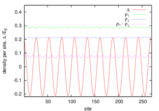
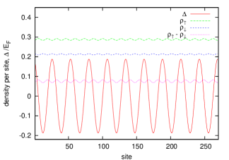
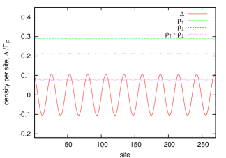
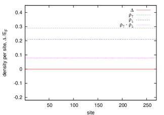
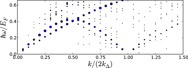
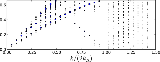
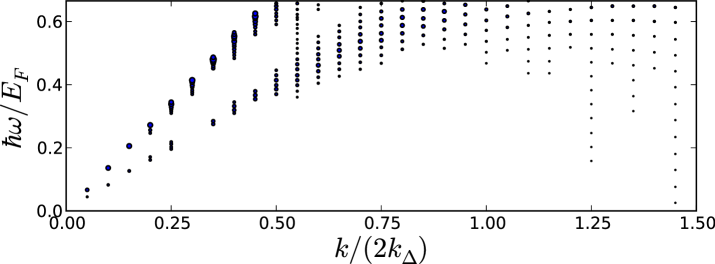
Figure 4: (Colour online) Response of a system at fixed chemical potential and different temperatures. The area of the circle is proportional to the amplitude of the response, as in Fig. 2. The polarisation is $p=0.15$, the interactions strength is $\gamma=1.5$ and there are roughly 135 particles. The temperatures are from left to right $T/T_{F}=0.0037,0.038,0.057,0.076$. Within our mean field theory calculation the oscillating order parameter disappears at a temperature $T/T_{F}=0.07$. Simultaneous with the disappearing of the oscillating order parameter the response around $k=k^{*}$ disappears.

III.3 Mean field theory versus exact theory

While the calculations we have presented are within RPA mean-field theory, as we now argue, the qualitative conclusions are valid more generally. In the above, the response spectrum was accounted for in terms of the broken translational and gauge symmetry of the mean-field state. As is well known, in a true 1D quantum system no continuous symmetries are broken. Thus, the broken (phase and translational) symmetries of the mean-field FFLO state can lead only to power-law decay of the respective correlation functions fflo_pairing_in_1d_opt_latt-rizzi_fazio08 . However, the qualitative features described above are the same as those expected from an exact treatment of the system. The transition from the (unpolarised) superfluid phase to the partially polarised phase is marked by the closing of the spin-gap, leading to a second gapless sound mode. This can be viewed as a Luttinger liquid representing the excess fermions Yang_inhomogeneous_sc_state_1d_01 . These excess particles have density $\rho_{\uparrow}-\rho_{\downarrow}$, and thus a Fermi wavevector $(k_{F,\uparrow}-k_{F,\downarrow})$. Thus, there are two gapless collective modes, arising from the fully paired particles, and the liquid of excess majority spin particles. Furthermore, as in the general theory of Luttinger liquids HaldaneJPhysC the spectral function of these excess majority spin particles will show gapless response at multiples of twice their Fermi wavevector. This is $2(k_{F,\uparrow}-k_{F,\downarrow})=4\pi/\lambda_{\Delta}$ which is precisely the wavevector $k^{*}$ at which one finds the gapless response in mean field theory. Thus, the qualitative features of the collective excitation spectrum obtained in mean-field theory are fully consistent with those expected for the exact system.

III.4 Temperature dependence of the collective modes

We now consider the temperature dependence of the collective response of the homogeneous system. For very low temperature ($T\lesssim 0.01T_{F}$) we find essentially the same response spectrum as for zero temperature. As the temperature of the system is increased and the order parameter disappears, the low energy response around $k=k^{*}$ also disappears, see Fig. 4. This can be explained by the fact that the BZ associated with the oscillating order parameter disappears. We also observe that as the temperature is increased $k^{*}$ no longer coincides with $2(k_{F,\uparrow}-k_{F,\downarrow})$. We note that thermally excited quasiparticles which do not contribute to the pairing can lead to this departure.

The results we have presented so far are purely within the collisionless regime. The collisionless regime describes the situation where the rate of quasiparticle collisions is much smaller than the frequency of the excitation. At zero temperature the system is always in the collisionless regime. On the other hand for non-zero temperature there are thermally excited quasiparticles. These may undergo collisions, thereby leading to a nonzero collision rate. As pointed out in Ref. theory_of_quantum_liquids1_nozieres_1966 , at nonzero temperature great care has to be taken when taking the limits $k\to 0$, $T\to 0$. These two limits do not commute. If first the temperature is taken to zero and subsequently $k$ is taken to zero, the system is in the collisionless regime. Sound modes in the collisionless regime correspond to zero sound. On the other hand if first $k\to 0$ and subsequently $T\to 0$ a hydrodynamic description is needed. In the hydrodynamic regime quasiparticles have time to scatter many times during the cycle of one collective oscillation and hence the system can be described in terms of local thermodynamic equilibria. In the crossover region no sound propagation is possible due to strong damping.

We have performed a simple analysis of the quasiparticle collision rate. In an infinite one-dimensional system no quasiparticle excitations can exist due to the divergent nature of the interactions; a Luttinger liquid HaldaneJPhysC description of the system is required quantum_physics_in_1d_giamarchi . All excitations are collective excitations. This manifests itself in an infinite quasiparticle scattering rate. On the other hand, in a finite system, the quasiparticle scattering rate is finite.

Using perturbation theory we find that in a system of size $L$, for $T\ll T_{F}$, the scattering rate of a quasiparticle with energy $k_{B}T$ is

$$\Gamma =\frac{g_{1d}^{2}k_{F}^{2}}{8\pi\hbar E_{F}}\frac{\mathrm{e}}{\mathrm{e}+1}\left[\frac{T}{T_{F}}+2\ln\left(\frac{\sqrt{3}}{4\pi}\frac{T}{T_{F}}k_{F}L\right)\right]\,.$$ (15)

In general for an infinite system the collisionless approximation will fail since $\Gamma$ diverges. In this case a hydrodynamic theory must be used. However, in practice all experimentally relevant systems are finite. Therefore there will be some temperature below which the system can be described as collisionless. For example, comparing the frequencies with the quasiparticle scattering rate for the system sizes used to compute Fig. 4, we find that in all apart from the four lowest frequency points for $T=0.076T_{F}$ and the lowest frequency point for $T=0.057T_{F}$ the systems are in the collisionless regime. We therefore expect the results presented in Fig. 4 to be qualitatively accurate for systems of this size.

For a given system of size $L$ the temperature below which the system can be considered collisionless may be found as follows. The lowest $k$ vector with which the system can be excited is given by $k=\frac{2\pi}{L}$. Fig. 3 suggests that for the parameters we are considering, the sound velocity $v$ is of the order of the Fermi velocity $v_{F}$. Then using the fact that the collisionless approximation will be valid up to approximately $\omega\approx\Gamma$ and using $\omega\approx kv_{F}$ we obtain that for a homogeneous system the maximum temperature $T_{m}$ for which the collisionless approximation is valid is given by

$$T_{m} \approx T_{F}\frac{4\pi}{\sqrt{3}k_{F}L}\mathrm{e}^{\frac{\pi^{4}(\mathrm{e}+1)}{\mathrm{e}}\frac{1}{k_{F}L\;\gamma^{2}}}$$ (16)

Here we we have only included the logarithmic dependence of $\Gamma$ on $T/T_{F}$ and not the linear part since the linear part is much smaller. Using eq. (16) we find that for the configurations in Fig. 4 the collisionless approximation is valid up to temperatures of around $T=0.05T_{F}$. For these systems this temperature coincides roughly with the temperature for which the FFLO phase disappears.

Above we argued that for the systems and temperatures studied in this paper we can work in the collisionless regime. The results of our calculations are valid in the regime in which interactions are assumed to be weak or moderately strong. On the other hand it has been reported that for strongly interacting 3D imbalanced Fermi systems one needs to consider the effects of collisions of quasiparticles even at experimentally achievable low temperatures coll_props_of_pol_FG-bruun-stringari08 ; collective_osc_of_imb_FG_polaron_nascimbene_salomon . There are some fundamental differences between those studies of 3D systems and the 1D systems of interest here. In the 3D systems, a spin imbalanced phase is stable only at relatively high polarisations (beyond the Chandrasekhar-Clogston limit). The collision rate is rapid until the temperature is small compared to the Fermi temperature of the minority component coll_props_of_pol_FG-bruun-stringari08 , which, in view of the large imbalance, can be a low energy scale. In contrast, in 1D the FFLO phase occupies a large region of parameter space, and it is possible to have this spin-imbalanced phase with much smaller polarisations when the Fermi energies for spin $\uparrow$ and $\downarrow$ atoms are of the same magnitude. One then expects that, for strong interactions, the relevant energy scale below which collisional scattering starts to become small is just the (typical) Fermi temperature. Our formulae (15) and (16) were derived using perturbation theory, so cannot be applied to determine the collisional scattering rate in the strongly interacting regime. We are not aware of a calculation of the thermal broadening of the collective modes for a strongly interacting spin-$\frac{1}{2}$ Fermi system of relevance here.

IV Trapped system

We now turn our attention to the experimentally more relevant case of the Fermi gas in a harmonic trap. Within the local density approximation (LDA) the possible ground state configurations for 1D Fermi gas at $T=0$ are known exactly from the Bethe ansatz phase_diag_of_str_int_pol_fg_1d_drummond07 ; orso_attr_fermi_gases_bethe_ansatz07 . There are only two possible configurations which are (a) a partially polarised phase in the middle, with a fully paired phase towards the edge and (b) a partially polarised phase in the middle, with a fully polarised phase towards the edge. Recently these configurations have also been observed in experiment spin_imbalance_in_a_1d_FG-Liao_Hulet_2009 . As shown by Ref. liu_drummond_07 Bogoliubov de Gennes theory reproduces these ground state configurations and it is in good qualitative agreement with the results of the exact solution combined with the LDA.

The low-frequency collective modes in a trap are the dipole and the breathing modes. Dipole modes are the lowest lying modes with odd parity around the centre of the trap. For $V_{\text{ext}}(x)=\frac{1}{2}m\omega_{0}^{2}x^{2}$ their frequencies in the non-interacting limit are given by $\omega=\omega_{0}$. Breathing modes are the lowest lying modes with even parity. They correspond to expansion and contraction of the atomic cloud. In the non-interacting limit their frequencies are given by $\omega=2\omega_{0}$. Both the dipole and breathing modes exist in two types: the spin and density modes. In the density modes the two atomic clouds move in phase whereas in the spin modes the two clouds move largely in anti-phase. Within these modes the density dipole mode has a special status. It is called the “Kohn mode” and corresponds to rigid body oscillations of the cloud about the centre of the trap. Its frequency $\omega$ is given by $\omega=\omega_{0}$ independent of the interaction strength.

We now investigate the accuracy of the single mode approximation for these low frequency modes.

IV.1 Single mode approximation

The single mode approximation (SMA) is an important tool in calculating collective mode frequencies. Together with sum rules it allows the calculation of collective mode frequencies from ground state properties alone. This can be done as follows: for an operator $\hat{F}$ the dynamic form factor $S(\omega)$ describes the strength of the transition from the ground state to state with energy $\hbar\omega$. $S(\omega)$ is given by sum_rules_and_giant_resonances_in_nuclei-lipparini_stringari89

$$S(\omega)=\sum_{k\not=0}\left|\left\langle k\right|\hat{F}\left|0\right\rangle\right|^{2}\delta(\omega-\omega_{k})$$ (17)

where $\left|k\right\rangle$ label the exact energy eigenstates of the system. We define the $p$th moment of the dynamic form factor as

$$m_{p}=\int_{0}^{\infty}S(\omega)\omega^{p}\,\mathrm{d}\omega\,.$$ (18)

Using sum rules it is possible to express $m_{1}$, $m_{3}$ and $m_{-1}$ as sum_rules_and_giant_resonances_in_nuclei-lipparini_stringari89

$$m_{1} =\frac{1}{2}\left\langle\left[\hat{F},\left[\hat{H},\hat{F}\right]\right]\right\rangle$$ (19)

$$m_{3} =\frac{1}{2}\left\langle\left[\left[\hat{F},\hat{H}\right],\left[\hat{H},\left[\hat{H},\hat{F}\right]\right]\right]\right\rangle$$ (20)

$$m_{-1} =-\frac{1}{2}\mbox{Im}\;\chi(\hat{F},\omega\to 0)$$ (21)

where $\chi(\hat{F},\omega)$ is the response function for the operator $\hat{F}$ at frequency $\omega$.

The SMA corresponds to the assumption that $S(\omega)$ is dominated by one sharp peak. Then the collective mode excited by the operator $\hat{F}$ has a frequency that is given by $\omega_{\hat{F}}=\omega_{p,p-2}=\sqrt{\frac{m_{p}}{m_{p-2}}}$ for any value of $p$. If the SMA is not exact, and more than one peak is present, one finds that $\omega_{p,p-2}>\omega_{q,q-2}$ for $p>q$ and this approach to finding the collective mode frequency using sum rules becomes less accurate. Nevertheless, $\omega_{p,p-2}$ still provides an upper bound for the lowest frequency collective mode. We use both $\omega_{1,-1}$ and $\omega_{3,1}$ to obtain upper bounds for the collective mode frequencies.

In order to investigate the dipole and the breathing modes we consider two sets of operators $\hat{F}$. For the dipole mode we consider $\hat{F}_{d}(\theta)=\cos\theta\sum_{i}x_{i}+\sin\theta\sum_{j}x_{j}$ where indices $i$ run over all the $\uparrow$ particles and $j$ over all the $\downarrow$ particles. For the breathing modes we consider $\hat{F}_{b}(\theta)=\cos\theta\sum_{i}x_{i}^{2}+\sin\theta\sum_{j}x_{j}^{2}$. $\hat{F}_{d}$ corresponds to applying linear potential $V_{\uparrow}(x)=x\cos\theta$ $,V_{\downarrow}(x)=x\sin\theta$ and $\hat{F}_{b}$ corresponds to applying a quadratic potential $V_{\uparrow}(x)=x^{2}\cos\theta$ $,V_{\downarrow}(x)=x^{2}\sin\theta$.

Here the single mode approximation amounts to assuming that the operator $\hat{F}(\theta)$ has at most two peaks in the response spectrum, each of which can be made to vanish by suitable choice of $\theta$. Hence the collective mode frequencies of the two associated modes can be obtained by maximising or minimising $\omega_{p,p-2}$. The lower frequency mode for each $\hat{F}$ is the density mode and the higher frequency mode is the spin mode.

For $\hat{F}_{d}$ we obtain in the continuum limit two values of $\theta$ which maximise or minimise $\omega_{3,1}$. For both $T=0$ and for $T>0$ these are $\theta_{\text{sd}}=-\arctan\frac{k_{F,\uparrow}}{k_{F,\downarrow}}$ for the spin dipole mode and $\theta_{\text{Kohn}}=\frac{\pi}{4}$ for the Kohn mode. For the breathing mode such simple analytical formulae for $\theta_{sb}$ (spin breathing mode) and $\theta_{db}$ (density breathing mode) which maximise/minimise $\omega_{p,p-2}$ could not be obtained. These can be obtained numerically though as has been done in Ref. phase_diag_of_str_int_pol_fg_1d_drummond07 , where the density breathing mode frequency was investigated using sum rules.

We have used our results to address the question: how accurate is the SMA in describing the results of the BdG+RPA approximation?

For all the modes mentioned above we find that the SMA is strictly speaking not correct, since $\omega_{3,1}\not=\omega_{1,-1}$. To gauge the accuracy of the SMA we have compared the prediction of the sum rule for $w_{1,-1}$ with the position of the peak in the response spectrum, see Fig. 5. We choose $\omega_{1,-1}$ because it gives higher accuracy results as it is not affected as much by low weight high frequency peaks as $\omega_{3,1}$ is. For the two density modes which are the lower frequency modes of the two operators $F_{d}$ and $F_{b}$ we find that there is very good agreement of the positions of the peak as obtained from the response spectrum and the SMA. For the density dipole mode (the Kohn mode) the sum rule calculation captures the position of the peak up to our numerical accuracy. For the density breathing mode the accuracy typically is about 1%. In the limit $p\to 1$ the single mode approximation becomes exact for these two modes as can easily be verified by evaluating eqs. (19) and (20) for a non-interacting gas.

However, for the spin modes the SMA is not as accurate. In particular for lower polarisations the frequency from the SMA estimate $\omega_{1,-1}$ can differ quite significantly from the position of the lowest frequency peak of the full spectrum. This is due to the presence of many small amplitude high frequency peaks. The increased weight of these high frequency peaks and the associated failure of the SMA is correlated with an increase in size of the fully paired region towards the edge of the cloud.

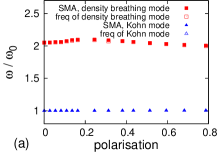
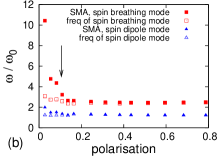
Figure 5: (Colour online) Calculation of the accuracy of the SMA using $\omega_{1,-1}$. (a): breathing modes and (b): spin modes. These plots are for $\gamma=1.2$ and different polarisations. For the density modes (a) the single mode approximation is very accurate. For the spin modes (b) the single mode approximation becomes inaccurate at small polarisations. The arrow indicates the point where the outside of the cloud goes from being fully paired ($p\lesssim 0.1$) to being fully polarised ($p\gtrsim 0.1$)

.

IV.2 Collective mode signature of the FFLO phase

As described in signature_of_fflo_first_paper_jonathan_nigel at $T=0$ we find a dramatic signature of the FFLO phase of a trapped Fermi gas when the spin-dipole mode is excited by a short-wavelength potential. When perturbing with potentials of the form (10) we find a large response of the spin dipole mode when the wavelength of the perturbing potential becomes $\lambda_{\Delta}/2$ . This response is independent of whether the ground state configuration is of type (a) or (b), that is whether the outside is fully paired or fully polarised. This response for these two types of system is shown in Figs. 6 and 7.

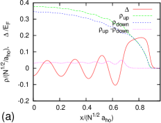
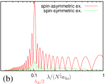
Figure 6: (Colour online.) Configuration with fully paired phase towards the edge of the trap. (a): densities and the value of the superfluid gap $\Delta$. (b): response of the spin-dipole mode to excitations of different wavelengths (arbitrary units). Here $p=0.048$, $\gamma=0.93$ (measured in centre), number of particles $N=290$, lattice spacing $a=3.3\cdot 10^{-3}N^{\frac{1}{2}}a_{ho}$ with $a_{ho}=\sqrt{\frac{\hbar}{m\omega_{0}}}$. The perturbing potential has a fixed amplitude, while the wavelength is varied.

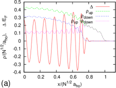
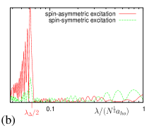
Figure 7: (Colour online.) Configuration with fully polarised phase towards the edge. Here $p=0.25$, $\gamma=1.5$, $a/(N^{\frac{1}{2}}a_{ho})=4.7\cdot 10^{-3}$, $N=143$ . Otherwise the same as Fig. 6.

This response can be understood in terms of coupling to the gapless modes at $k=\frac{4\pi}{\lambda_{\Delta}}=k^{*}$ of the homogeneous system (see Fig.2 and Sec. III.2). A small deviation from $k^{*}$ (of the order the inverse system size) allows mixing of this mode to the spin-dipole mode, causing the response at $k^{*}$ to be apparent in the dipolar motion of the atomic cloud.

As in the untrapped system, at very low temperatures the system behaves in the same way as for $T=0$. With increasing temperature the oscillating gap $\Delta$ disappears. Along with it the sharp response at the wavelength $\lambda_{\Delta}/2$ disappears, see Fig. 8. There are a few additional noteworthy points. As the temperature is increased the number of modes which can be excited increases. This can lead to the splitting of, for example, the spin dipole mode into two near degenerate sub modes. For yet higher temperature further fractionalisation of the modes occurs, see Fig. 8. At intermediate temperatures (Fig. 8) an oscillating gap can still be made out but the peak in the response of the spin dipole mode is strongly attenuated, which may increase the difficulty of finding the FFLO phase. An example of a system which at $T=0$ is fully paired towards the outside is given in Fig. 8, but the case where the outside is fully polarised at $T=0$ is qualitatively similar.

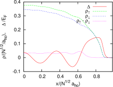
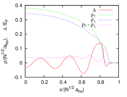
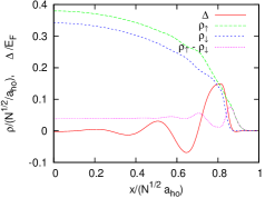
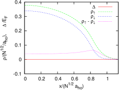
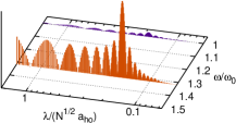
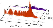
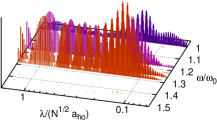
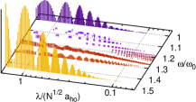
Figure 8: (Colour online) Response of a system (for which at $T=0$ the outside is fully paired) to a periodic potential of wavelength $\lambda$ and freqency $\omega$. There are 173 particles, $\gamma=0.93$, $p$ varies from 0.05 to 0.09. The temperature is $T=0.0005T_{F}$, $T=0.005T_{F}$, $T=0.02T_{F}$ and $T=.106T_{F}$. For the lowest temperature the spin-dipole frequency is $\omega=1.31\omega_{0}$. The sharp peak at the spin-dipole frequency at $\lambda/(N^{1/2}a_{ho})\approx 0.2$ is the signature of the FFLO phase. At higher temperatures, this sharp response disappears and additional excitations emerge. The case where the outside is fully polarised towards the edge at $T=0$ is qualitatively the same.

As in the homogeneous case discussed in Sec. III.2 our calculation is performed in the collisionless regime. Using eq. (16) and the LDA by taking the system size to be roughly the size of the cloud we find that the collisionless regime should be valid up to a temperature of $T/T_{F}\approx 0.03$. This is slightly lower than in Sec. III.4 since the system size is larger. Nevertheless, the three configurations in Fig. 8 with an FFLO phase are still in the collisionless regime.

Most results presented in this paper are for values of $\gamma\approx 1-1.6$ where the mean-field theory we use is expected to be accurate. (For the groundstate, this is confirmed by comparisons with exact results liu_drummond_07 .) We have performed calculations with larger $\gamma$, in the range of $\gamma=2.2-3.8$, and find qualitatively the same results. While we cannot trust the quantitative results of mean-field theory in regimes of strong interactions, particularly at unitarity, we believe that the qualitative results remain valid. In particular, the key signature of the FFLO phase that we predict relies only on the commensurability between the wavelength of the perturbing potential and the intrinsic periodicity of the FFLO phase, and is expected to be robust.

IV.3 Experimental considerations

Recently experiments have produced true 1D ultracold Fermi gases as an array of 1D tubes spin_imbalance_in_a_1d_FG-Liao_Hulet_2009 . By changing the coupling between the tubes it is possible to tune continuously between a 3D system and a true 1D system. The experimental results show evidence for the appearance of a partially polarised phase in a regime of parameters consistent with the theoretical expectations for the phase associated with the FFLO state. Probing the collective modes in the manner described in this paper would lead to direct evidence of the intrinsic modulation of the FFLO phase.

Observing the signature of the FFLO phase in experiments in this way requires the ability to create a variable wavelength optical lattice. This can be done using the technique used by Ref. ex_spectrum_of_bec_steinhauer_davidson02 . Although the signal appears for a spin-symmetric perturbation, the signal is clearer for spin-asymmetric perturbations. Thus, any spin-dependence of the optical lattice will enhance the ability to distinguish the peaks associated with the oscillation of $\Delta$ from the background peaks. For Bosons (⁸⁷Rb) potentials with spin-dependence have been created by Ref. cohenrent_transp_of_neut_atoms_in_spin_dep_opt_latt_mandel_bloch03 , and would be ideally suited to this purpose. There are additional complications associated with applying spin-dependent potentials to ⁶Li due to increased loss rates resulting from the application of the potentials bragg_scattering_and_spin_struc_fac_in_2cmpt_gases-carusotto2006 . As discussed in Ref. bragg_scattering_and_spin_struc_fac_in_2cmpt_gases-carusotto2006 it is nevertheless in principle possible to set up these potentials. There are two natural ways to find the response of the spin-dipole mode. One way is to follow the approach of the calculation precisely, and make the strength of the optical lattice time dependent, as in Ref. transitino_from_strongly_int_1d_sf_to_MI_stoferle_Kohl_Esslinger04 . The spin-dipole mode can then be selectively excited by bringing the temporal oscillation of the lattice in resonance with the spin-dipole mode. Alternatively a static periodic potential can be applied to the system and the system allowed to equilibrate. Subsequently this potential is abruptly switched off (similar to the approach used in Ref. altmeyer07 ). This will excite collective modes of many frequencies from which the response of the spin-dipole mode can be obtained by Fourier transform.

In quasi_1d_pol_fermi_SFs-parish-huse07 it is maintained that in order to see the FFLO phase by in situ imaging it is advantageous to induce coupling between the different 1D tubes in order to align the phases of the FFLO state between the different tubes. However, for the method we are considering this should not be necessary. The response of the system depends on the wavelength with which the system is excited and on $\lambda_{\Delta}$. Only one laser is used to create the optical lattice with which the system is excited which implies that the wavelength with which the system is excited is the same for all tubes. Therefore, as long as the wavelength of the FFLO phase is approximately the same between different tubes, the response will be be small or large for the same excitation wavelengths. As a result it should be possible just to work with very weakly coupled or uncoupled 1D tubes and still see this effect.

One experimental difficulty in detecting the FFLO phase in systems of the type studied in Ref. spin_imbalance_in_a_1d_FG-Liao_Hulet_2009 – which is shared by all probes of the intrinsic periodicity of the FFLO phase – is the inhomogeneity across the many 1D tubes. Due to the different positions of the tubes in the atomic trap, different tubes will have different chemical potentials. In general this will lead to different values of $\lambda_{\Delta}$ in different tubes. Since the large response occurs for perturbations with $\lambda=\lambda_{\Delta}/2$ only those tubes which meet the condition on $\lambda_{\Delta}$ will show a strong response. If all the tubes can only be imaged as a whole it is therefore desirable to work in a regime where $\lambda_{\Delta}$ varies minimally between different tubes. As pointed out by Ref. quasi_1d_pol_fermi_SFs-parish-huse07 it is possible to choose a point in the phase diagram where $\frac{\,\mathrm{d}{\lambda_{\Delta}}}{\,\mathrm{d}{\mu}}=\frac{\,\mathrm{d}^{2}{\lambda_{\Delta}}}{\,\mathrm{d}{\mu}^{2}}=0$. At this point the value of $\lambda_{\Delta}$ should be the same over a large range of tubes in the centre of the system.

Our method provides a very elegant way to overcome the effects of inhomogeneity, if in situ imaging can allow individual or a small collection of 1D tubes to be resolved. This will allow one to relax the condition of having any intertube tunneling and being at a special point in the phase diagram. By exciting the whole system with a given wavelength $\lambda$, only those tubes with $\lambda_{\Delta}\simeq 2\lambda$ will have their spin-dipole oscillations excited. Tubes with the same value for $\lambda_{\Delta}$ lie on concentric cylinders around the trap centre. Thus, if imaging of the cloud has sufficient resolution to identify which tubes are oscillating, one should see response from tubes that lie on a cylindrical region around the axis of the trap. Changing the wavelength $\lambda$ will change the radius of this cylindrical region. In this way the FFLO wavelength could be studied as a function of the position of the 1D tube in the trap. This approach is only limited by the power to resolve the 1D tubes.

IV.4 Modulation of the coupling constant

We have investigated the response of the one-dimensional Fermi gas to a modulation of the coupling constant. This is an interesting perturbation to consider, since using Feshbach resonances it is relatively easy to implement a uniform modulation of the coupling constant experimentally. Recently it was also found, that in a lattice system parametric modulation can be achieved by modulating the lattice depth parametric_resonance_in_1d_fermionic_sys-graf-mariani .

Modulations of the coupling constant couple to density differences. The FFLO state has a density difference that shows quasi-periodic spatial oscillations, as explained above. Hence it is interesting to ask if the response of the system is sensitive to the appearance of the ordering characteristic of the FFLO phase.

Within linear response the modulation of the coupling constant of the form $U=U_{0}+\delta U(t)$ leads to a perturbation of the form

$$\delta W_{i,\sigma}(t) =\frac{\delta U(t)}{U_{0}}V^{int}_{i,\sigma}$$ (22)

$$\delta\Delta_{i}(t) =\frac{\delta U(t)}{U_{0}}\Delta_{i}$$ (23)

and hence the response to a modulation of the coupling constant is amenable to our RPA calculation.

We have studied the response of the trapped gas to modulations of the coupling constant, focusing on the regime of low frequencies. Since a modulation of the coupling constant does not break reflection symmetry about the centre of the trap it can only excite trap modes of even parity. As a result the lowest frequency modes which can be excited are the breathing modes.

We find that the nature of the response of the system depends strongly on whether the system is in the configuration (a), which is fully paired toward the edge and exhibits an FFLO phase in the centre, or in the configuration (b), which is fully polarised towards the edge. When the outside is fully polarised the majority of the response weight is at the lower frequency density breathing mode and there is little or no response at the higher frequency spin breathing mode. On the other hand, in the case where the outside is fully paired and there is an FFLO phase in the centre the situation is reversed. Most of the weight of the responses on the high-frequency spin breathing mode. See Fig. 9.

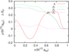
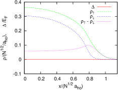
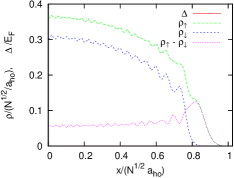
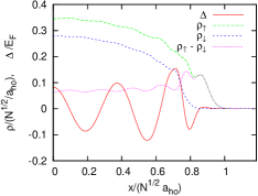
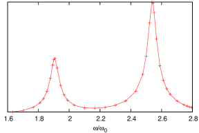
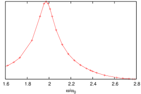
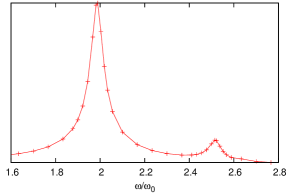
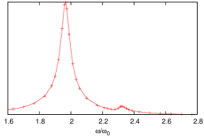
Figure 9: (Colour online) Response of a trapped system to a modulation of the coupling constant. Whenever the outside is fully paired the weight of the response of the spin breathing mode (the higher frequency mode) is larger than that of the density breathing mode (lower frequency). All are for $\gamma=1.2$. From left to right we have a system at $T=0$ which is fully paired towards the edge (73 particles), a high-temperature system ($T=0.1$ , 74 particles), a system where the order parameter $\Delta$ was set to 0 (74 particles) and a system with FFLO phase but which is fully polarised at the edge (67 particles). The bottom row shows the respective responses.

While the nature of the response is senstive to the global distribution of particles, whether or not an FFLO phase is present makes little difference to the response spectrum. We must therefore conclude that there is no clear signal of the presence of the FFLO phase in the collective mode spectrum excited by a modulation of the coupling constant. On the other hand the collective mode spectrum appears to be sensitive to whether the outside region of the cloud is fully paired or fully polarised.

V conclusion

To conclude, we have investigated the collective mode spectrum of the imbalanced Fermi gas. The FFLO phase can be detected due to the formation of a characteristic periodicity of the densities. This makes it possible to use short wavelength perturbations which couple to the intrinsic periodicity of the FFLO phase in order to excite long wavelength responses which are easy to measure in experiment. This signal in the collective mode spectrum persists up to the temperature where the FFLO phase disappears. We also investigated the accuracy of the single mode approximation. We found that it works very well for density modes, but not as well for spin modes. Finally, we found that a modulation of the coupling constant results in a collective mode spectrum which allows us to distinguish long wavelength characteristics of the density profile but not short wavelength characteristics, as are associated with the FFLO phase.

- (1) I. Bloch, J. Dalibard, and W. Zwerger, Rev. Mod. Phys. 80, 885 (2008).
- (2) S. Giorgini, L. P. Pitaevskii, and S. Stringari, Rev. Mod. Phys. 80, 1215 (2008).
- (3) G. Partridge et al., Science 311, 503 (2006).
- (4) M. Zwierlein, A. Schirotzek, C. Schunck, and W. Ketterle, Science 311, 492 (2006).
- (5) A. Larkin and Y. Ovchinnikov, Zh. Eksp. Teor. fiz. 47, 1136 (1964), [Sov. Phys. JETP 20, 762 (1965)].
- (6) P. Fulde and R. A. Ferrell, Phys. Rev. 135, A550 (1964).
- (7) E. Lifshitz and L. Pitaevskii, Statistical Physics Part 2 (Pergamon Press, Oxford, 1980).
- (8) D. E. Sheehy and L. Radzihovsky, Annals of Physics 322, 1790 (2007).
- (9) G. Orso, Phys. Rev. Lett. 98, 070402 (2007).
- (10) H. Hu, X.-J. Liu, and P. D. Drummond, Phys. Rev. Lett. 98, 070403 (2007).
- (11) A. E. Feiguin and F. Heidrich-Meisner, Phys. Rev. B 76, 220508(R) (2007).
- (12) M. M. Parish, S. K. Baur, E. J. Mueller, and D. A. Huse, Phys. Rev. Lett. 99, 250403 (2007).
- (13) G. G. Batrouni, M. H. Huntley, V. G. Rousseau, and R. T. Scalettar, Phys. Rev. Lett. 100, 116405 (2008).
- (14) A. Lüscher, R. M. Noack, and A. M. Läuchli, Phys. Rev. A 78, 013637 (2008).
- (15) Y. Liao et al., Spin-Imbalance in a One-Dimensional Fermi Gas, arXiv:0912.0092v1, 2009.
- (16) M. R. Bakhtiari, M. J. Leskinen, and P. Törmä, Phys. Rev. Lett. 101, 120404 (2008).
- (17) J. M. Edge and N. R. Cooper, Physical Review Letters 103, 065301 (2009).
- (18) C. Lobo, A. Recati, S. Giorgini, and S. Stringari, Phys. Rev. Lett. 97, 200403 (2006).
- (19) S. Nascimbène et al., Phys. Rev. Lett. 103, 170402 (2009).
- (20) A. Lazarides and B. Van Schaeybroeck, Phys. Rev. A 77, 041602(R) (2008).
- (21) B. Van Schaeybroeck, J. Tempere, and A. Lazarides, Trapped Two-Dimensional Fermi Gases with Population Imbalance, arXiv:0911.0984v1, 2009.
- (22) X. W. Guan, M. T. Batchelor, C. Lee, and M. Bortz, Phys. Rev. B 76, 085120 (2007).
- (23) T. Iida and M. Wadati, Journal of the Physical Society of Japan 77, 024006 (2008).
- (24) J.-S. He, A. Foerster, X. W. Guan, and M. T. Batchelor, New Journal of Physics 11, 073009 (17pp) (2009).
- (25) E. Zhao et al., Phys. Rev. Lett. 103, 140404 (2009).
- (26) C. N. Yang, Phys. Rev. Lett. 19, 1312 (1967).
- (27) M. Gaudin, Phys. Lett. A 24, 55 (1967).
- (28) M. Takahashi, Thermodynamics of One-Dimensional Solvable Models (Cambridge University Press, Cambridge, UK, 1999).
- (29) X.-J. Liu, H. Hu, and P. D. Drummond, Phys. Rev. A 76, 043605 (2007).
- (30) G. M. Bruun and B. R. Mottelson, Phys. Rev. Lett. 87, 270403 (2001).
- (31) K. Yang, Phys. Rev. B 63, 140511(R) (2001).
- (32) T. Mizushima, M. Ichioka, and K. Machida, Journal of the Physical Society of Japan 76, 104006 (2007).
- (33) X.-J. Liu, H. Hu, and P. D. Drummond, Phys. Rev. A 78, 023601 (2008).
- (34) T. Koponen, J.-P. Martikainen, J. Kinnunen, and P. Törmä, Physical Review A (Atomic, Molecular, and Optical Physics) 73, 033620 (2006).
- (35) D. Forster, Hydrodynamic Fluctuations, Broken Symmetry, and Correlation Functions (W. A. Benjamin, Reading, Mass., 1975).
- (36) M. Rizzi et al., Phys. Rev. B 77, 245105 (2008).
- (37) F. D. M. Haldane, Journal of Physics C: Solid State Physics 14, 2585 (1981).
- (38) P. Nozières and D. Pines, The theory of quantum liquids (Perseus Books, New York, 1966).
- (39) T. Giamarchi, Quantum Physics in One Dimension (Oxford University Press, Oxford, 2004).
- (40) G. M. Bruun et al., Phys. Rev. Lett. 100, 240406 (2008).
- (41) E. Lipparini and S. Stringari, Physics Reports 175, 103 (1989).
- (42) J. Steinhauer, R. Ozeri, N. Katz, and N. Davidson, Phys. Rev. Lett. 88, 120407 (2002).
- (43) O. Mandel et al., Phys. Rev. Lett. 91, 010407 (2003).
- (44) I. Carusotto, Journal of Physics B: Atomic, Molecular and Optical Physics 39, S211 (2006).
- (45) T. Stöferle et al., Phys. Rev. Lett. 92, 130403 (2004).
- (46) A. Altmeyer et al., Phys. Rev. A 76, 033610 (2007).
- (47) C. D. Graf, G. Weick, and E. Mariani, Parametric resonance and spin-charge separation in 1D fermionic systems, arXiv:0910.4123v2, 2009.