Chapter 1 Lattice QCD in Collision
Shoji Hashimoto^1,2
(1) KEK Theory Center, Institute of Particle and Nuclear Studies, High Energy Accelerator Research Organization (KEK), Tsukuba 305-0801, Japan
(2) School of High Energy Accelerator Science, the Graduate University for Advanced Studies (Sokendai), Tsukuba 305-0801, Japan

Abstract

In this talk, I present my personal view on the status of lattice QCD calculations. I emphasize the role played by the chiral perturbation theory ($\chi$PT) in analyzing the lattice data of various physical quantities, including chiral condensate, topological susceptibility, and pion mass and decay constant. I then discuss on the status of determination of fundamental parameters and other quantities of phenomenological interest.

1. Introduction

It was already more than 30 years ago that Quantum Chromodynamics (QCD) was proposed as the fundamental theory of strong interaction. Since then, there have been an enormous number of experimental data that support QCD including its quantum effects. Those experiments are essentially measuring perturbative aspects of QCD at high energy, while the non-perturbative dynamics at low energy still remains as a difficult problem. Solving QCD is difficult mainly because its vacuum is so complicated. There is no single dominant gauge field configuration; it is not completely random either. Since hadrons are floating on this vacuum, an understanding of the QCD vacuum is a prerequisite to calculate hadron properties starting from first principles.

Lattice QCD is one of the methods to regularize ultraviolet divergences in QCD. Unlike the commonly used dimensional regularization, whose definition involves perturbation theory, lattice QCD is valid in both ultraviolet and infrared regimes. As the regulated theory is mathematically well-defined, direct numerical calculation of the path integral that defines QCD is possible. Thus, lattice QCD provides a powerful method for first-principles calculation of QCD including its non-perturbative dynamics at low energy. It requires huge computational resources, especially to incorporate the fermion loop effects in the path integral. Since 1980s, lattice QCD has been using the high-end supercomputers available at the time. It is remarkable that researchers of lattice QCD have even developed machines that lead the entire supercomputing.

The state-of-the-art of lattice QCD simulations could be summarized as follows: “Realistic simulation of QCD to study the static properties of hadrons is now feasible”. It means that the inclusion of up, down and strange sea quarks has become a standard at small enough lattice spacing ($a\lesssim$ 0.1 fm) on large enough volume ($L\gtrsim$ 2.5 fm) to hold a single hadron. The low-energy hadron spectrum, for instance, has been well reproduced by several lattice groups.

Although the recent progress of lattice QCD is so impressive, it still has many limitations. One of those is the multi-scale problems. The scales that may enter in the QCD phenomena are widely ranged: up and down quark masses ($\sim$ 5 MeV), strange quark mass ($\sim$ 100 MeV), the QCD scale ($\sim$ 300 MeV), charm quark mass ($\sim$ 1.5 GeV), and bottom quark mass ($\sim$ 4.5 GeV). Treating light quarks requires more computational costs that grows as $1/m_{q}^{2-3}$ with $m_{q}$ the light quark mass; reducing the lattice spacing to treat heavy quarks needs more resources that typically scales as $1/a^{7}$ with $a$ the lattice spacing. Therefore, the best strategy for practical applications is to use “effective theories” such as the chiral perturbation theory ($\chi$PT) for light quarks and the heavy quark effective theory (HQET) for heavy quarks. The light and heavy quark masses for which these effective theories are valid have to be carefully investigated using lattice QCD calculations.

This talk is not a comprehensive review of the field. Rather, I would like to present my personal view of the status of lattice QCD. I start the discussion from a study of the fundamental property of the QCD vacuum in Section 2. Then I summarize the calculations of some interesting phenomenological quantities of light hadrons with special emphasis on the convergence property of the chiral expansion (Section 3). Determination of the fundamental parameters of QCD, such as the strong coupling constant and quark masses is of particular importance, that I discuss in Section 4. My discussion on heavy flavor physics is brief (Section 5). My summary and perspective are in the last section.

2. Chiral symmetry breaking

2.1. Chiral symmetry and lattice QCD

One of the fundamental properties on the QCD vacuum is the spontaneous breaking of chiral symmetry. Even before QCD, many important properties of low-energy hadrons, such as the GMOR relation and other soft pion theorems, were discovered based on the PCAC relation and current algebra. From the modern perspective, they are derived from the chiral effective theory, which is constructed assuming the spontaneous chiral symmetry breaking. For the thorough understanding of strong interaction, it is therefore a crucial step to establish a link between QCD and chiral effective theory.

Chiral symmetry of course plays a key role in the understanding of chiral symmetry breaking. In the flavor non-singlet sector of chiral symmetry, pions arise as the Nambu-Goldstone boson associated with the spontaneous symmetry breaking, while in the flavor-singlet sector the chiral symmetry is violated by the axial anomaly and is related to the topology of non-Abelian gauge theory. There are near-zero modes of quarks associated with the topological excitations; their accumulation in the vacuum leads to the symmetry breaking in the flavor non-singlet sector as indicated by the Banks-Casher relation [1]. Therefore, the initial setup to study the chiral symmetry breaking should preserve the flavor singlet and non-singlet chiral symmetries.

There is a problem in realizing the chiral symmetry on the lattice. The conventional Wilson-type fermions violate the chiral symmetry at the action level, and the discrimination between the physical effect of symmetry breaking and the lattice artifact is not clear. On the other hand, the staggered fermions have a chiral symmetry but break the flavor symmetry. With these lattice fermions, the continuum limit has to be taken before analyzing the data using the continuum chiral effective theory.

The domain-wall [2, 3, 4] and overlap [5, 6] fermions solve this problem in a theoretically clean manner. Since they satisfy a modified version of chiral symmetry at finite lattice spacing [7], the continuum-like axial-Ward-Takahashi identities are hold on the lattice. (The chiral symmetry is exact for the overlap fermion; for the domain-wall fermion the chiral symmetry is restored in the limit of infinite size of the fifth dimension, but small violation remains in practical simulations.) This means that the soft-pion theorems are all satisfied on the lattice just as in the continuum theory, as far as the chiral symmetry is spontaneously broken. The use of $\chi$PT is therefore justified at any finite lattice spacing $a$. (For the Wilson and staggered fermions, one has to include the terms that represent the violation of chiral symmetry.) Although the numerical cost is substantially high compared to the Wilson or staggered fermions, these fermion formulation should therefore be used when the chiral symmetry is crucial.

The spontaneous chiral symmetry breaking is probed by the chiral condensate $\langle\bar{q}q\rangle$. Its lattice calculation is challenging because the scalar density operator $\bar{q}q$ has a power divergence of the form $m_{q}/a^{2}$ as the cutoff $1/a$ goes to infinity. The massless limit has to be taken to obtain physical result. (When the chiral symmetry is violated from the outset as in the Wilson-type fermions, the divergence is even stronger $\sim 1/a^{3}$.) On the other hand, the condensate vanishes in the massless limit, when the space-time volume is kept finite. Therefore, the proper order of the limits is to take the infinite volume limit first and then the massless limit, which is called the thermodynamical limit.

2.2. Spectral density and chiral condensate

The problem of the ultraviolet divergence can be avoided by focusing on low-lying eigenmode spectrum of the Dirac operator. As indicated by the Banks-Casher relation [1], the chiral symmetry breaking is induced by an accumulation of low-lying eigenstates of quark-antiquark pair

$$\lim_{m\to 0}\lim_{V\to\infty}\rho(\lambda=0)=\frac{\Sigma}{\pi},$$ (1)

where $\rho(\lambda)$ denotes the eigenvalue density of the Dirac operator, $\rho(\lambda)\equiv(1/V)\sum_{k}\langle\delta(\lambda-\lambda_{k})\rangle$. The expectation value $\langle\cdots\rangle$ represents an ensemble average and $k$ labels the eigenvalues of the Dirac operator on a given gauge field background. On the right hand side of (1), $\Sigma$ is the chiral condensate, $\Sigma=-\langle\bar{q}q\rangle$, evaluated in the massless quark limit. In the free theory, we expect a scaling $\rho(\lambda)\sim\lambda^{3}$ for a dimensional reason and thus $\rho(0)=0$. The relation (1) implies that the spontaneous chiral symmetry breaking characterized by non-zero $\Sigma$ is related to the number of near-zero modes in a given volume.

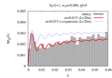
Fig. 1: Spectral density of the Dirac operator calculated by the JLQCD collaboration (histogram). The curve represents a next-to-leading order $\chi$PT calculation [11]. The pion mass is around 300 MeV and the system in the $p$-regime.

Based on $\chi$PT, more detailed forms of $\rho(\lambda)$ at finite $\lambda$, $V$ and $m$ have been obtained. This provides a theoretical basis to control the scaling under the change of these parameters. A recent simulation of the JLQCD collaboration gave the spectral density with 2+1 flavors of dynamical overlap fermions [8]. (An earlier analysis is in [9, 10]). One of the results is shown in Figure 1, which is obtained at lattice spacing $\sim$ 0.11 fm and lattice volume $\sim$ (1.8 fm)${}^{3}\times$(5.4 fm). The plot compares the result with a $\chi$PT calculation at the next-to-leading order [11]. The shape of the spectrum is nicely reproduced, and the height determines the chiral condensate at the given quark mass.

A similar analysis is attempted using the Wilson fermion in [12]. Due to the explicit violation of chiral symmetry, the spectrum of the near-zero modes is distorted. Relatively larger eigenvalues are, therefore, mainly used in the comparison with $\chi$PT.

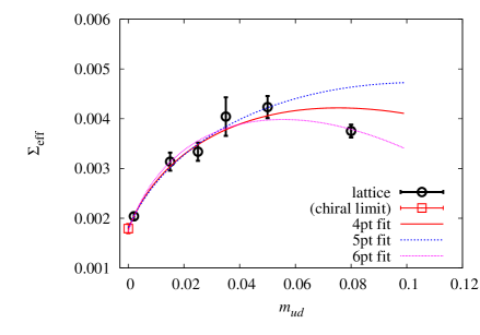
Fig. 2: Chiral condensate as a function of sea quark mass. Results from the JLQCD collaboration.

An extrapolation of the chiral condensate $\Sigma(m_{ud},m_{s})$ to the chiral limit of up and down quark masses is shown in Figure 2. The lattice data of the JLQCD collaboration show a curvature, which is essentially a pion-loop effect as predicted by $\chi$PT [13]

$$\Sigma(m_{ud},m_{s})=\Sigma(0,m_{s})\times$$ (2)

$$\left[1-\frac{3M_{\pi}^{2}}{32\pi^{2}F^{2}}\ln\frac{M_{\pi}^{2}}{\mu^{2}}+\frac{32L_{6}M_{\pi}^{2}}{F^{2}}\right].$$

The data point close to the chiral limit, which is in the so-called $\epsilon$-regime, is helpful to identify this curvature. A preliminary result in the chiral limit of up and down quarks is $\Sigma^{\overline{\mathrm{MS}}}(0,m_{s};\mathrm{2~{}GeV})=[243(4)(^{+16}_{-\ 0})\mathrm{~{}MeV}]^{3}$.

2.3. Topological susceptibility

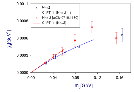
Fig. 3: Topological susceptibility $\chi_{t}$ as a function of sea quark mass. Lattice data are from [15, 16].

The topology of gauge field configuration plays a key role in the accumulation of the near-zero modes. The amount of topological excitations is measured by the topological susceptibility $\chi_{t}=\langle Q^{2}\rangle/V$, where $Q$ is the global topological charge in a given volume $V$. An expectation from $\chi$PT is that $\chi_{t}$ behaves as $\chi_{t}=m\Sigma/N_{f}$ with $m$ the quark mass of $N_{f}$ degenerate flavors [14]. (There is also a formula for non-degenerate quark masses.) A lattice result by the JLQCD and TWQCD collaboration [15, 16] obtained with the overlap fermion is shown in Figure 3. The results from two-flavor and 2+1-flavor QCD are well described by $\chi$PT. This precise calculation was made possible by a new method to calculate $\chi_{t}$ through a topological charge density correlation on gauge configurations at fixed global topological charge [17].

Through these studies, the spontaneous breaking of chiral symmetry is well established using the first-principles calculation of lattice QCD. The exact chiral symmetry provided by the overlap fermion played a crucial role there. The $\chi$PT is confirmed to be valid near the chiral limit for fundamental quantities such as the chiral condensate and topological susceptibility. The next question would be how much the region of $\chi$PT is extended towards wider applications and larger values of pion masses/momenta.

3. Light hadron phenomenology

3.1. Convergence of chiral expansion

At Lattice 2002, the annual conference on lattice field theory, there was a panel discussion on the issue of chiral extrapolation of lattice data [18]. The problem at that time was that the curvature due to the chiral logarithm of the form $m_{\pi}^{2}\ln m_{\pi}^{2}$ was not visible in lattice data for any physical quantity. This was mainly because the quark mass in the dynamical fermion simulations at that time was too large that pion mass was above 500 MeV, which is presumably out of the range of $\chi$PT. This lead to a large systematic error in the chiral extrapolation.

Since then, by the development of algorithms and machines, the pion mass in the lattice simulations has been reduced down to 200–300 MeV. For a summary of recent large-scale simulations, see the plenary talk by Scholz at Lattice 2009 [19]. Now, it is therefore the time to investigate the convergence property of the chiral expansion.

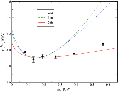
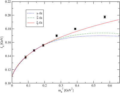
Fig. 4: Comparison of chiral expansion in terms of $x$, $\hat{x}$ and $\xi$. The plots represent $m_{\pi}^{2}/m_{q}$ (left) and $f_{\pi}$ (right). Fits of the three lightest data points with the NLO ChPT formulae (3) and (4) are shown. Results are from [20].

The $\chi$PT provides a systematic expansion in terms of small $m_{\pi}^{2}$ and $p^{2}$, but the region of convergence of this chiral expansion is not known a priori. With the exact chiral symmetry, the test is conceptually cleanest, since no additional terms to describe the violation of chiral symmetry has to be introduced. (With other fermion formulations, this is not the case as already noticed. The unknown correction terms are often simply ignored.)

For the pion mass $m_{\pi}$ and decay constant $f_{\pi}$ the expansion is given as

$$\frac{m_{\pi}^{2}}{m_{q}} = 2B\left[1+\frac{1}{2}x\ln x+c_{3}x+O(x^{2})\right],$$ (3)

$$f_{\pi} = f\left[1-x\ln x+c_{4}x+O(x^{2})\right],$$ (4)

where $m_{\pi}$ and $f_{\pi}$ denote the quantities after the corrections while $m$ and $f$ are those at the leading order. The expansions (3) and (4) may be written in terms of either $x\equiv 2m^{2}/(4\pi f)^{2}$, $\hat{x}\equiv 2m_{\pi}^{2}/(4\pi f)^{2}$, or $\xi\equiv 2m_{\pi}^{2}/(4\pi f_{\pi})^{2}$ (we use a notation of $f_{\pi}$ = 131 MeV). They all give an equivalent description at this order, while the convergence behavior may depend on the expansion parameter.

Among other works, I use our own data (by the JLQCD and TWQCD collaborations) for a discussion here. Figure 4 shows the comparison of different expansion parameters in two-flavor QCD [20]. The fit curves are obtained by fitting three lightest data points with the three expansion parameters, which provide equally precise description of the data in the region of the fit. If we look at the heavier quark mass region, however, it is clear that only the $\xi$-expansion gives a reasonable function and others miss the data points largely. This clearly demonstrates that at least for these quantities the convergence of the chiral expansion is much better with the $\xi$-parameter than with the other conventional choices. This is understood as an effect of resummation of the chiral expansion by the use of the “renormalized” quantities $m_{\pi}^{2}$ and $f_{\pi}$. In fact, only with the $\xi$-expansion we could fit the data including the kaon mass region with the next-to-next-to-leading order (NNLO) formulae [20].

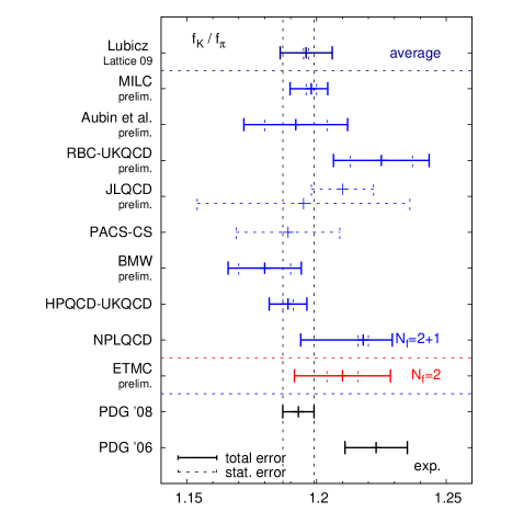
Fig. 5: $f_{K}/f_{\pi}$ from various lattice groups. A plot from E. Scholz [19]. References for individual data can be found there. In the plot, PDG’08 is from the experimental data of leptonic kaon decay, assuming $|V_{us}|=0.2255(19)$.

With the NLO formulae (like those in (3) or (4)), the convergence of the chiral expansion is marginal in the kaon mass regime. In fact, some groups concluded not to use the SU(3) $\chi$PT for the kaon sector but use the SU(2) formula with the strange quark treated as a heavy particle. This corresponds to an expansion in terms of $m_{ud}/m_{s}$ and is a theoretically consistent treatment, though the predictive power of $\chi$PT is lost to some extent. A summary of the results for $f_{K}/f_{\pi}$ from a review talk at Lattice 2009 by Scholz [19] is shown in Figure 5. Different groups take different strategies on the treatment of strange quark in the chiral fit, i.e. SU(2) or SU(3), NLO or NNLO. At the level of the error of order $\pm$0.02, the results are in agreement.

3.2. Kaon semi-leptonic form factor

Whether the strange quark can be treated within the SU(3) $\chi$PT is an important issue, since the main sources of phenomenological information for kaon physics relies on $\chi$PT. For instance, the determination of a CKM matrix element $|V_{us}|$ uses the semileptonic decays $K\to\pi\ell\nu$. It is made precise because the relevant form factor $f^{+}(q^{2})$ is normalized to 1 at $q^{2}=0$ in the degenerate SU(3) limit. The deviation from there is estimated using the SU(3) $\chi$PT [21]. Even the lattice calculations use its formula as a guide to fit the data. The recent result by the RBC-UKQCD collaboration with 2+1 flavors of domain-wall fermions [22] is $f^{+}(0)=0.964(5)$, which is consistent with 0.961(8) of the early phenomenological work [21].

3.3. Neutral kaon mixing

Results for $B_{K}$, the bag parameter to characterize the $K^{0}-\bar{K}^{0}$ mixing, has been made very precise and stable by recent lattice calculations. The recent results in 2+1-flavor QCD are: $\hat{B}_{K}$ = 0.720(13)(37) with 2+1 flavors of domain-wall fermions [23], 0.724(8)(28) with domain-wall valence quarks over 2+1 flavors of staggered sea quarks [24]. Even including two-flavor calculations using overlap [25] and twisted-mass [26] fermions, all the dynamical lattice calculations give consistent results. The average given by Lubicz at Lattice 2009 [27] is $\hat{B}_{K}=0.731(7)(35)$.

With the 5% error, $B_{K}$ is no longer the dominant uncertainty in drawing the constraint on the CKM unitarity triangle from the indirect CP violation parameter $|\epsilon_{K}|$. Since $|\epsilon_{K}|$ is related to the $(\rho,\eta)$ parameters of the CKM unitary triangle as $|\epsilon_{K}|\propto B_{K}A^{2}\eta(c_{1}+c_{2}A^{2}(1-\rho))$ ($c_{1}$ and $c_{2}$ are known constants), the uncertainty in $|V_{cb}|\equiv A\lambda^{2}$ is now more important, as emphasized in [28].

For the lattice calculations related to the kaon physics, I also refer the readers to a recent comprehensive review by Boyle at the Kaon09 conference [29].

4. Fundamental parameters

Next, I discuss the recent determinations of fundamental parameters in QCD, i.e. the strong coupling constant and quark masses.

4.1. Strong coupling constant

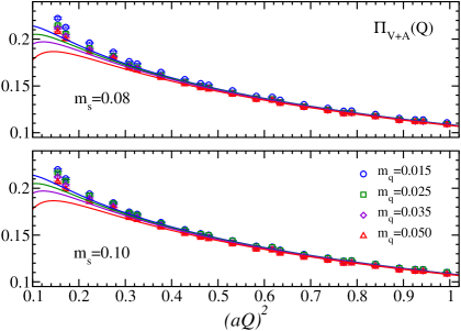
Fig. 6: Fit of the vacuum polarization function on the lattice with continuum perturbative calculation. Data from the JLQCD collaboration with 2+1 flavors of dynamical overlap fermions [33].

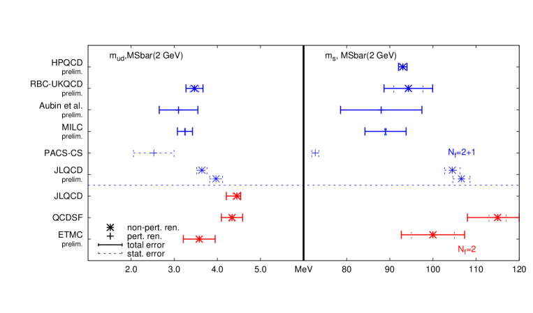
Fig. 7: Summary of the quark mass determinations from the lattice. A plot from Scholz [19]. References for individual data can be found there. Results with perturbative and non-perturbative renormalization factors are distinguished by pluses and starts, respectively.

The determination of the strong coupling constant is equivalent to an input of the lattice scale $1/a$. This is because, for a given lattice with a bare coupling constant $\alpha_{s}^{\mathrm{lat}}$, it gives the running of the coupling constant $\alpha_{s}^{\mathrm{lat}}(a^{-1})$. But, in order to obtain the value in more familiar definitions, such as the one in the $\overline{\mathrm{MS}}$ scheme, one has to convert the result using perturbation theory as $\alpha_{s}^{\overline{\mathrm{MS}}}(\mu)=Z(\mu a)\alpha_{s}^{\mathrm{lat}}(a^{-1})$. Therefore, precise determination requires a good control of systematic errors in the perturbative matching factor $Z(\mu a)$. This is the reason that the previous lattice calculation by the HPQCD collaboration [30, 31] employed an automated perturbative calculation methods to calculate two-loop contributions on the lattice.

Recently, new methods have been proposed. They are based on a physical quantity which is sufficiently short-distance and is calculable in both continuum and lattice theories. A well-known example is the Adler function, which is a derivative of the vacuum polarization function $D(Q^{2})\equiv-Q^{2}d\Pi_{V}(Q^{2})/dQ^{2}$. Since this quantity does not have an ultraviolet divergence, the perturbative calculation in the continuum theory using the dimensional regularization can be applied for the lattice data without modifications except for possible discretization effects. Therefore, one may fit the lattice data using the continuum formula known to three-loops (or even four-loops for the leading term) supplemented by an operator product expansion in $1/Q^{2}$. Then, one can directly determine $\alpha_{s}^{\overline{\mathrm{MS}}}(\mu)$ [32]. The fit of lattice data in 2+1-flavor QCD is shown in Figure 6 for different light quark masses. A preliminary result $\alpha_{s}(M_{Z})=0.1181(8)(^{+4}_{-2})(^{+5}_{-6})$ has an error which is comparable to the previous best lattice calculation, 0.1183(8) [30, 31].

A closely related method is the use of the charmonium two-point function. By taking an appropriate moment in the coordinate space, the ultraviolet divergence is removed and the lattice data can be directly fitted with a corresponding continuum calculation. The result is $\alpha_{s}(M_{Z})=0.1174(12)$ [34]. With this method, one can also determine the charm quark mass at the same time [34].

Overall, the lattice calculation now provides the most precise determination of the strong coupling constant. Along the lines of the recent calculations, further improvement is expected.

4.2. Quark masses

Light quark masses can be extracted with pion and kaon masses as inputs. Therefore, the results depend on the fit functions (SU(2) or SU(3), NLO or NNLO) and the mass range used in the analysis of pion and kaon masses. Since the pole mass of quarks is not well defined due to confinement, one has to use a renormalization scheme given at short distances such as the $\overline{\mathrm{MS}}$ scheme. Conversion from the lattice bare quark mass is done using perturbation theory or partially using some non-perturbative methods. The errors with purely perturbative method could be significantly underestimated, as the coefficients of higher order terms are not known a priori. The results summarized in Figure 7 (from the review by Scholz [19] at Lattice 2009) should be viewed with these caveats in mind. Since many results appeared only recently, the understanding of these systematics will be achieved in the coming years. I expect that the error is reduced to 2–5% in the near future.

The isospin breaking, or the up and down quark mass ratio, cannot be determined solely from the QCD calculation, as the electromagnetic effect gives a substantial contribution. For instance, the charged and neutral mass difference of pion is dominated by the QED effect, which has to be subtracted to determine $m_{u}-m_{d}$. There is an attempt to identify the QED effect using the Weinberg-type sum rule [35]: $m_{\pi^{\pm}}^{2}-m_{\pi^{0}}^{2}\propto\alpha_{EM}\int_{0}^{\infty}dQ^{2}Q^{2}[\Pi_{V}(Q^{2})-\Pi_{A}(Q^{2})]$. Here, the difference of the vacuum polarization functions in the vector and axial-vector channels is involved, which means that this mass difference is triggered by the spontaneous chiral symmetry breaking. With exact chiral symmetry, lattice calculation of $\Pi_{V}(Q^{2})-\Pi_{A}(Q^{2})$ is possible [36]. Another interesting method to calculate the QED effect is a simulation of the whole QCD+QED system [37, 38]. Then one can also calculate the charged and neutral kaon mass difference, which is useful to study the amount of the violation of the Dashen’s theorem $m_{K^{\pm}}^{2}-m_{K^{0}}^{2}=m_{\pi^{\pm}}^{2}-m_{\pi^{2}}^{2}$ [39]. More striking application would be the mass difference between proton and neutron, as it is related to a big question of why the matters in Nature are stable. For a recent analysis, see [38].

5. Heavy flavors

The biggest motivation to consider the heavy quark flavors is to put constraints on the CKM unitarity triangle. Since the experiments of $B$ meson decays have been dramatically improved over the last several years, the required precision for the lattice calculation has become high. Namely, to be interesting, the lattice calculation for the decay constants, bag parameters, and form factors has to be typically as precise as 5% or even better, which is a challenge for the lattice QCD community.

For instance, determination of the CKM matrix elements $|V_{cb}|$ and $|V_{ub}|$ can be done through inclusive or exclusive decay modes. The inclusive determination uses perturbative calculation relying on the quark-hadron duality assumption, while the exclusive determination requires the lattice calculation of the form factors. So far, the precision of the inclusive determination is slightly better for both $|V_{cb}|$ and $|V_{ub}|$, as far as the error is taken as a face value. See a summary plot in Figure 8 made by Van de Water [28]. More importantly, the inclusive and exclusive determinations are inconsistent with each other at around 2$\sigma$ level. In order to understand this discrepancy, more precise calculations and experiments are required.

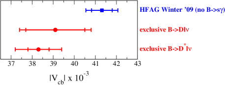
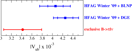
Fig. 8: Inclusive and exclusive determinations of $|V_{cb}|$ (top panel) and $|V_{ub}|$ (bottom panel). Plats are taken from Van de Water [28]. The lattice data are those in [40].

Since the Compton wavelength of heavy quarks is too short to treat on the lattice that is available with present computational power, one has to use some effective theory. The idea is to factor out a trivial heavy quark mass dependence $e^{-im_{Q}t}$ from physical amplitudes; remaining terms are organized as an expansion in terms of $1/m_{Q}$. The effective theories realize this in a language of effective lagrangians, and it is also possible to construct a lattice version. The problem is that the effective theory has many parameters that have to be determined so that it reproduces the original QCD. In many cases, the matching of these parameters is done by perturbation theory, with which neglected higher order corrections become a source of systematic error. Non-perturbative parameter matching has also be attempted [41], but is not common as it required dedicated study for each choice of lattice gauge and fermion actions. (For an introductory article on heavy quarks on the lattice, see [42]).

On the other hand, as the available computational resources increase, it has also become possible to directly simulate heavy quarks with the lattice spacing kept as small as possible. It is feasible only in the charm quark mass region, and an extrapolation is necessary toward bottom quark mass. In particular a variant of the staggered fermion (the HISQ action) [43] has been found to be useful to minimize discretization effects. Because the staggered fermion has a chiral symmetry (at a price of broken flavor symmetry), the order of discretization effect is limited to $O(a^{2})$, $O(a^{4})$, …; the HISQ action is designed to remove the leading $O(a^{2})$ effect so that the remaining error is $O(a^{4})$ at the tree level. Other non-chiral fermions have the errors of $O(a)$, $O(a^{2})$, …; the removal of the lowest order effect leaves the $O(a^{2})$ effect, which is still substantial.

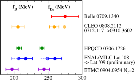
Fig. 9: $D_{(s)}$ meson decay constant. Experimental data and lattice calculations are compared. A plot from Van de Water [28]. CLEO and FNAL/MILC data have been updated in 2009; the solid lines are the latest results.

In order to demonstrate how precision is crucial in heavy flavor phenomenology, I show a summary plot of the calculation of $D_{(s)}$ meson decay constant $f_{D_{(s)}}$ in Figure 9. Although there are three recent lattice calculations, the result of the HPQCD collaboration [44] using the HISQ action has an order of magnitude smaller error quoted and thus dominates the lattice calculations. If it is compared with experiments, one may conclude that there is a significant discrepancy in $f_{D_{s}}$, which triggered theorists to consider some new physics models that may explain this [45, 46]. Therefore, it is very important to have other calculations that reach this level of precision with different lattice fermion formulations. This needs two or three more years in my opinion.

6. Summary and perspective

The development of supercomputers was initiated in 1980s, and an exponential growth of the computational power has been continued since then. The rate is about a factor of 10 in 5 years over the last 25–30 years, and still no trend of speed-down is observed. This, of course, has driven the rapid improvement of lattice calculations. Until 1990s, only the quenched calculations were possible, and the results were subject of uncontrolled systematic errors. Large-scale dynamical fermion simulations were started at around late 90s, and with lots of efforts to improve algorithms and techniques the simulations in a realistic setup have become feasible recently. This means that the lattice calculation can now produce real predictions from QCD for many interesting quantities.

Theoretically, the biggest achievement in the last 10–20 years in lattice field theory is the formulation of lattice fermions with chiral symmetry. It removed a large class of limitations of lattice calculations. Indeed, spontaneous chiral symmetry breaking and related phenomena can now be directly simulated in lattice QCD.

These facts promise a wider range of applications of lattice QCD. The coverage of this talk has been limited, but lattice QCD may be useful in many other areas of particle and nuclear physics. They include nucleon structure, spin physics, exotic hadrons, muon $g-2$, flavor ($B$, $D$, and $K$) physics, heavy ion physics, and even dark matter search or neutrino interactions — nearly all the subjects that were covered by the Physics in Collision conference. Lattice QCD is your friend!

Acknowledgements

I would like to thank Enno Scholz and Ruth Van de Water for allowing me to use the plots they prepared for their Lattice 2009 plenary talks. I also thank the members of JLQCD/TWQCD for fruitful collaborations. The author is supported in part by Grant-in-aid for Scientific Research (No. 21674002).

Bibliography

- [1] T. Banks and A. Casher, Nucl. Phys. B 169, 103 (1980).
- [2] D. B. Kaplan, Phys. Lett. B 288, 342 (1992) [arXiv:hep-lat/9206013].
- [3] Y. Shamir, Nucl. Phys. B 406, 90 (1993) [arXiv:hep-lat/9303005].
- [4] V. Furman and Y. Shamir, Nucl. Phys. B 439, 54 (1995) [arXiv:hep-lat/9405004].
- [5] H. Neuberger, Phys. Lett. B 417, 141 (1998) [arXiv:hep-lat/9707022].
- [6] H. Neuberger, Phys. Lett. B 427, 353 (1998) [arXiv:hep-lat/9801031].
- [7] M. Luscher, Phys. Lett. B 428, 342 (1998) [arXiv:hep-lat/9802011].
- [8] H. Fukaya et al. [JLQCD collaboration], arXiv:0911.5555 [hep-lat].
- [9] H. Fukaya et al. [JLQCD Collaboration], Phys. Rev. Lett. 98, 172001 (2007) [arXiv:hep-lat/0702003].
- [10] H. Fukaya et al., Phys. Rev. D 76, 054503 (2007) [arXiv:0705.3322 [hep-lat]].
- [11] P. H. Damgaard and H. Fukaya, JHEP 0901, 052 (2009) [arXiv:0812.2797 [hep-lat]].
- [12] L. Giusti and M. Luscher, JHEP 0903, 013 (2009) [arXiv:0812.3638 [hep-lat]].
- [13] J. Gasser and H. Leutwyler, Annals Phys. 158, 142 (1984);
- [14] H. Leutwyler and A. V. Smilga, Phys. Rev. D 46 (1992) 5607.
- [15] S. Aoki et al. [JLQCD and TWQCD Collaborations], Phys. Lett. B 665, 294 (2008) [arXiv:0710.1130 [hep-lat]].
- [16] T. W. Chiu et al. [JLQCD and TWQCD Collaborations], PoS LAT2008 (2008) 072; arXiv:0810.0085 [hep-lat].
- [17] S. Aoki, H. Fukaya, S. Hashimoto and T. Onogi, Phys. Rev. D 76, 054508 (2007) [arXiv:0707.0396 [hep-lat]].
- [18] C. Bernard, S. Hashimoto, D. B. Leinweber, P. Lepage, E. Pallante, S. R. Sharpe and H. Wittig, Nucl. Phys. Proc. Suppl. 119, 170 (2003) [arXiv:hep-lat/0209086].
- [19] E. E. Scholz, arXiv:0911.2191 [hep-lat].
- [20] J. Noaki et al. [JLQCD and TWQCD Collaborations], Phys. Rev. Lett. 101, 202004 (2008) [arXiv:0806.0894 [hep-lat]].
- [21] H. Leutwyler and M. Roos, Z. Phys. C 25, 91 (1984).
- [22] P. A. Boyle et al., Phys. Rev. Lett. 100, 141601 (2008) [arXiv:0710.5136 [hep-lat]].
- [23] D. J. Antonio et al. [RBC Collaboration and UKQCD Collaboration], Phys. Rev. Lett. 100, 032001 (2008) [arXiv:hep-ph/0702042].
- [24] C. Aubin, J. Laiho and R. S. Van de Water, arXiv:0905.3947 [hep-lat].
- [25] S. Aoki et al. [JLQCD Collaboration], Phys. Rev. D 77, 094503 (2008) [arXiv:0801.4186 [hep-lat]].
- [26] P. Dimopoulos et al., PoS LATTICE2008, 271 (2008) [arXiv:0810.2443 [hep-lat]].
- [27] V. Lubicz, plenary talk at Lattice 2009.
- [28] R. S. Van de Water, arXiv:0911.3127 [hep-lat].
- [29] P. A. Boyle, arXiv:0911.4317 [hep-ph].
- [30] Q. Mason et al. [HPQCD Collaboration and UKQCD Collaboration], Phys. Rev. Lett. 95, 052002 (2005) [arXiv:hep-lat/0503005].
- [31] C. T. H. Davies, K. Hornbostel, I. D. Kendall, G. P. Lepage, C. McNeile, J. Shigemitsu and H. Trottier [HPQCD Collaboration], Phys. Rev. D 78, 114507 (2008) [arXiv:0807.1687 [hep-lat]].
- [32] E. Shintani et al. [JLQCD Collaboration and TWQCD Collaboration], Phys. Rev. D 79, 074510 (2009) [arXiv:0807.0556 [hep-lat]].
- [33] T. Onogi et al. [JLQCD Collaboration], in PoS LATTICE2009 (2009).
- [34] I. Allison et al. [HPQCD Collaboration], Phys. Rev. D 78, 054513 (2008) [arXiv:0805.2999 [hep-lat]].
- [35] T. Das, G. S. Guralnik, V. S. Mathur, F. E. Low and J. E. Young, Phys. Rev. Lett. 18 (1967) 759.
- [36] E. Shintani et al. [JLQCD Collaboration], Phys. Rev. Lett. 101, 242001 (2008) [arXiv:0806.4222 [hep-lat]].
- [37] R. Zhou, T. Blum, T. Doi, M. Hayakawa, T. Izubuchi and N. Yamada, arXiv:0810.1302 [hep-lat].
- [38] T. Izubuchi, PoS (KAON09) 034.
- [39] R. F. Dashen, Phys. Rev. 183, 1245 (1969).
- [40] C. Bernard et al., Phys. Rev. D 79, 014506 (2009) [arXiv:0808.2519 [hep-lat]].
- [41] J. Heitger and R. Sommer [ALPHA Collaboration], JHEP 0402, 022 (2004) [arXiv:hep-lat/0310035].
- [42] S. Hashimoto and T. Onogi, Ann. Rev. Nucl. Part. Sci. 54, 451 (2004) [arXiv:hep-ph/0407221].
- [43] E. Follana et al. [HPQCD Collaboration and UKQCD Collaboration], Phys. Rev. D 75, 054502 (2007) [arXiv:hep-lat/0610092].
- [44] E. Follana, C. T. H. Davies, G. P. Lepage and J. Shigemitsu [HPQCD Collaboration and UKQCD Collaboration], Phys. Rev. Lett. 100, 062002 (2008) [arXiv:0706.1726 [hep-lat]].
- [45] B. A. Dobrescu and A. S. Kronfeld, Phys. Rev. Lett. 100, 241802 (2008) [arXiv:0803.0512 [hep-ph]].
- [46] A. S. Kronfeld, arXiv:0912.0543 [hep-ph].