Direct Measurement of Kirkwood-Rihaczek distribution for spatial properties of coherent light beam

Abstract

We present direct measurement of Kirkwood-Rihaczek (KR)distribution for spatial properties of coherent light beam in terms of position and momentum (angle) coordinates. We employ a two-local oscillator (LO) balanced heterodyne detection (BHD) to simultaneously extract distribution of transverse position and momentum of a light beam. The two-LO BHD could measure KR distribution for any complex wave field (including quantum mechanical wave function) without applying tomography methods (inverse Radon transformation). Transformation of KR distribution to Wigner, Glauber Sudarshan P- and Husimi or Q- distributions in spatial coordinates are illustrated through experimental data. The direct measurement of KR distribution could provide local information of wave field, which is suitable for studying particle properties of a quantum system. While Wigner function is suitable for studying wave properties such as interference, and hence provides nonlocal information of the wave field. The method developed here can be used for exploring spatial quantum state for quantum mapping and computing, optical phase space imaging for biomedical applications.

I Introduction

Optical phase-space tomography kim99 ; wax96 ; wax01 ; Reil05 ; walmsley96 ; cheng99 ; smith05 ; mukamel03 is an optical method for characterizing spatial properties of light fields/photons. The Kirkwood (K(x,p)) kirkwood33 and Wigner (W(x,p)) wigner32 distribution functions were originally proposed in the studies of quantum statistics and thermodynamic for almost classical ensembles. The Kirkwood distribution ($\psi(x)\psi^{*}(p)e^{-ixp}$)has been rediscovered by Rihaczek rihaczek68 for use in the theory of time-frequency analysis of classical signals. The Wigner function is more popular than the KR function because it has some unique properties such as negative values, real and symmetry. It can be obtained through tomograph methods and applicable to problems in phase space transport equation such as Liouville equation sjohn96 . The Wigner function was first introduced in optical light field by Bastiaans bastiaans78 ; bastiaans97 to analysis spatial properties of an optical Gaussian beam. In quantum optics, the quantum mechanical wave function cannot be measured in principle. The wave function or quantum state of a physical system can be best represented by the Wigner function. Vogel and Risken vogel89 had theoretically proposed how quadrature amplitudes of nonclassical light fields can be represented in Wigner distribution by tomograph methods. Raymer smithey93 ; lvovsky09 ; raymer94 ; mcalister95 ; beck93 has pioneered the tomography measurement of Wigner function for quadrature amplitudes of squeezed light, spatial properties and time-frequency properties of coherent light (coherent state with large mean photon number).

In most quantum information experiment, a single spatial mode of electromagnetic field is generally used and considered kolobov06 ; kolobov99 . Quantum fluctuations of light at different spatial points in the transverse plane of the light beam have to be taken into account. Kolobov and Sokolov kolobov86 ; kolobov89 ; kolobov89b ; kolobov89c ; kolobov91 have studied in detail the possibility of local squeezing in a spatial mode of light beam. Multimode spatial modes would cause information processing and computing errors. The property of multimode squeezed light which allows us to increase the sensitivity beyond the shot-noise limit, could create many interesting new applications in optical imaging, high-precision optical measurements, optical communications and optical information processing. However, one has to employ a dense array of photodetectors to observe multimode squeezed states.

The phase space distributions from the Glauber Cahill s-parameterized class of quasi-distributions cahil69 that contain the Wigner function, the Glauber Sudarshan P-representation sudarshan63 , and the Husimi husimi40 or the Q-representation, have been widely used as powerful phase space tools. However, most of tomograph methods are not involving direct measurement of these quasi-quantum distribution functions. These distributions are usually reconstructed from the raw data, where numerical and mathematical transformation discrepancies may have made these distributions doubtfully representing the true states. The direct measurement of these distributions are desirable to represent the true quantum state. It is well understood that tomograph methods developed for these distributions can be used for any complex wave fields regardless of classical or quantum origin smith07 ; lvovsky09 . In this perspective, we use wave field to represent quantum mechanical wave function and coherent light field.

The KR distribution for any quantum state in a generalized form has been introduced wodkiewicz03b . The hydrogen atom has been investigated using the Kirkwood$-$Rihaczek phase space representation wodkiewicz03 . It has been pointed out that the KR distribution may not suitable for a ”rotated state”. The Wigner function for a rotated state is just simply the rotated Wigner function. This is the basis property in tomography method applied in reconstruction of Wigner function. However, this simple relation does not hold for KR function. Tomograph methods (Radon Transform) are not suitable for KR function. It is worth noting that position and momentum distributions of wave field can be obtained through the KR distribution such as $\int K(x,p)dp=|\psi(x)|^{2}$ and $\int K(x,p)dx=|\psi(p)|^{2}$, respectively. These properties are similar to Wigner function. Moreover, the complex conjugated KR can be directly measured through a two-LO technique kim99 , not like Wigner function which is reconstructed from experimental data using quantum tomographic methods. Phase-space distribution functions especially Wigner function can unravel unique quantum properties such as entanglement of correlated systems schleich06 ; wodkiewicz99 , negative parts of phase-space plots schleich01 , and the phase space sub-Planck structures of quantum interference zurek06 ; zurek01 . The KR is relatively unexplored for quantum fields.

Spatial coherence of light sources is necessary for achieving efficient coupling into fiber systems for quantum communication, and also for biomedical imaging in image-guide intervention brezinski08 . From a quantum-mechanical perspective, spatial degree of freedom of a photon is another optical quantum realization for encoding information such as spatial qubits kolobov06 . Full characterization of arbitrary, continuous spatial states of photons is important for understanding the concept of the photon wave function smith07 . Wigner function for an ensemble of identically prepared photons in the transverse spatial modes can be completely used to characterize the transverse spatial state of the ensemble. The KR distributions are relatively unexplored for spatial properties of wave fields. In the second quantization of quantum mechanics, electric field is written as operator in term of harmonic oscillator basis, that is, position and momentum operators. The spatial property of the electric field perpendicular to the propagation direction is described by mode functions. The mode function in x or p coordinate is a description of probability amplitude to find a photon at transverse position x or transverse momentum p, respectively. The field operator $\hat{a}(x)$ corresponding to the mode function will provide mean field $\langle\hat{a}(x)\rangle$ and quantum noise $\triangle\hat{a}(x)$ in an optical detection scheme. In this work, distribution of x and p of a coherent wave field is measured by using a two-LO balanced heterodyne detection. Mean value measurement of the wave field $\langle\hat{a}(x)\rangle$ at a configuration space will provide classical-like feature regardless the origin (classical or quantum light) of the measured field. Variance measurement of the wave field $\triangle\hat{a}(x)$ will provide quantum feature of the light field. For coherent state with low mean photon number or large mean photon number, the variance for the quantum noise of wave field is constant loudon00 , that is, position or momentum independence. Therefore, the measurement method we have developed for coherent light is also applicable to coherent state, making them a useful testing ground for quantum imaging and mapping for information processing and quantum communication. Recently, EPR entanglement in spatial coordinate has been demonstrated by mixing an optical coherent light beam with squeezed light pklam08 . However, their measurements had involved displacement and ’tilt’ (momentum or angular) of a whole optical beam, not the transverse amplitude and phase structure of the optical beam. There is no approach in continuous variable quantum mechanics to measure the Wigner function or density matrix of spatial properties of EPR entangled beams. The optical technique and procedure presented in this paper could provide detail studies of phase-space physics in quantum metrology through sub-Planck phase-space structures in the Wigner function, and also discrete Wigner function for quantum mapping.

Phase-space distributions are used to represent quantum-mechanical operators in exploring phase-space quantum effects and quantum-classical correspondence. Quantum algorithms for measuring KR and Wigner distributions have been developed saraceno04 ; saraceno02 . Discrete phase space distribution has been suggested to show potential advantages in quantum computing especially quantum mapping. Quantum algorithm can be simply thought of as a quantum map acting in a Hilbert space of finite dimensionality. Specifically, algorithms become interesting in the large N limit  i.e., when operating on many qubits!. For a quantum map, this is the semiclassical limit where regularities may arise in connection with its classical behavior. These semiclassical properties may provide hints to develop new algorithms and ideas for novel physics simulations.

In this paper, we demonstrate direct measurement of the KR distribution for a wave field with Gaussian mode function of $TEM_{oo}$. Linear transformation from KR distribution to Wigner, P and Q-distribution are also plotted to show the fundamental differences in theirs respective. Second, a superposition of two spatially separated coherent light beams is used for discussing the phase-space interferences in these distributions. We show that complex conjugated KR distributions for spatial properties of wave fields can be determined by use of a novel two-LO balanced heterodyne detection scheme kim99 . The technique measures $\mathcal{K}^{*}(x,p)=<\mathcal{E}^{*}(x)\mathcal{E}(p)>e^{ixp}$, which can be written as $S_{R}+iS_{I}$. A lock-in-amplifier is used to measure the $S_{R}$ and $S_{I}$ with respect to relative phase setting of a reference signal at $0^{\circ}$ and $90^{\circ}$, respectively. By changing the lock-in-amplifier reference phases such as $0^{\circ}$ and $-90^{\circ}$, the system will measure $\mathcal{K}(x,p)$. However, we keep the lock-in-amplifier with reference phases at $0^{\circ}$ and $90^{\circ}$ for all measurements in this paper. There is no different in physics implied by wave field in KR or complex conjugated KR representation. The two-LO heterodyne technique was originally designed for biomedical imaging, that is for optical phase space coherence tomography of the light transmitted through or reflected from biological tissue. Now, we use this measurement to explore the properties of one particle wave mechanics or wave field through KR, Wigner, P- and Q- distributions. The technique can be used to measure any complex spatial wave fronts such as divergence and convergence, and phase-conjugated properties of wave field wax01 ; Reil05 . The $\mathcal{K}^{*}(x,p)$ can be easily transformed to Wigner function by using a linear transformation where the Radon transform is not required. The advantage of KR is it contains local information of the wave field. If there is no wave field presents at a configuration space (x,p), then there will be no distribution at the (x,p). It serves better for optical imaging in biomedical application such as to characterize the cell structure. We will illustrate this spatial property of KR distribution and compare it with Wigner function, P- and Q- distributions. In the two-LO balanced heterodyne detection, we use a local oscillator (LO) field comprising a coherent superposition of a tightly focused LO Gaussian beam of $TEM_{oo}$ and a highly collimated LO Gaussian beam of $TEM_{oo}$. This scheme permits independent control of the $x$ and $p$ resolution, permitting concurrent localization of $x$ and $p$ with a variance product that surpasses the minimum uncertainty limit associated with Fourier-transform pairs. Quantum mechanics did not allow simultaneously measurement of x and p of a wave field. However, simultaneous measurement in distribution of x and p for a wave field is allowed.

II Characteristic Function Approach

In this section, the characteristic function method will be used to transform the characteristic function of KR distribution to Wigner, P- and Q- distributions. The characteristic functions in term of harmonic oscillator basis will be used through out this paper because it is more revelent to spatial properties of coherent wave fields. Since we directly measure the complex conjugated of KR distribution, we will discuss how the measured results can be used to obtain Wigner, P- and Q- distributions. We start with the characteristic function for the complex conjugated of the KR distribution in term of coherent state representation, as given by,

$$\mathcal{M}_{KR}(\beta,\beta^{*})=Tr(\rho e^{-|\beta^{2}-\beta^{*2}|/4}e^{i\beta\hat{a}^{{\dagger}}+i\beta^{*}\hat{a}}).$$ (1)

where ($\beta$, $\beta^{*}$) are the Fourier conjugate pairs for ($\alpha$, $\alpha^{*}$)the eigenvalues of $\hat{a}$ and $\hat{a}^{*}$, respectively. The interesting feature of this characteristic function in the Fourier plane $M_{KR}(\beta,\beta^{*})$ is the trace of displacement operator $\mathcal{\hat{D}}(\beta)$ followed by squeezing operator $\mathcal{S}(1/2)$. The absolute of $|\beta^{2}-\beta^{*2}|/4$ just to avoid the confusion of other forms of definition that are, $\beta\rightarrow i\beta$ and $\beta^{*}\rightarrow-i\beta^{*}$. The complex conjugated of KR distribution in the $(\alpha,\alpha^{*})$ plane can be obtained through,

$$\mathcal{K}^{*}(\alpha,\alpha^{*})=\frac{1}{\pi^{2}}\int d^{2}\beta e^{-i\beta\alpha^{*}-i\beta^{*}\alpha}\mathcal{M}_{KR}(\beta,\beta^{*}).$$ (2)

The $\mathcal{K}^{*}(\alpha,\alpha^{*})$ can be transformed to Wigner, P- and Q- distributions in term of $(\alpha,\alpha^{*})$ through the relationships of the characteristic functions, such that,

$$\mathcal{M}_{KR}(\beta,\beta^{*})=e^{-|\beta^{2}-\beta^{*2}|/4}\mathcal{M}_{W}(\beta,\beta^{*})$$ (3)

where,

$$\mathcal{M}_{W}(\beta,\beta^{*})=e^{-|\beta|^{2}/2}\mathcal{M}_{P}(\beta,\beta^{*})=e^{|\beta|^{2}/2}\mathcal{M}_{Q}.$$ (4)

The characteristic function for Wigner function is given by,

$$\mathcal{M}_{W}(\beta,\beta^{*})=Tr(\rho e^{i\beta\hat{a}^{{\dagger}}+i\beta^{*}\hat{a}}).$$ (5)

The P- and Q- representations are related to the characteristic function of Wigner function through normal ordering and anti-normal ordering of $(\hat{a},\hat{a}^{*})$.

In our experiment, we measure spatial properties of a wave field in term of position and momentum coordinates (x,p). The $\mathcal{K}^{*}(x,p)$ can be obtained from Eq. (1) and Eq. (2) using the variables,

$$\hat{a}=\frac{1}{\sqrt{2}}(\hat{x}+i\hat{p});\hat{a}^{{\dagger}}=\frac{1}{\sqrt{2}}(\hat{x}-i\hat{p})$$

$$\beta=\frac{1}{\sqrt{2}}(\sigma+i\tau);\beta^{*}=\frac{1}{\sqrt{2}}(\sigma-i\tau)$$

$$\sigma=\frac{1}{\sqrt{2}}(x+ip);\sigma^{*}=\frac{1}{\sqrt{2}}(x-ip).$$ (6)

Then, the following terms,

$$e^{i\beta\hat{a}^{{\dagger}}+i\beta^{*}\hat{a}}=e^{i\sigma\hat{x}+i\tau\hat{p}};$$

$$e^{-|\beta^{2}-\beta^{*2}|/4}=e^{-i\sigma\tau/2};$$

$$e^{-i\beta\sigma^{*}-i\beta^{*}\sigma}=e^{-i\sigma x-i\tau p},$$ (7)

are obtained. The $\mathcal{K}^{*}(x,p)$ can be written as,

$$\mathcal{K}^{*}(x,p)=\int d\sigma d\tau e^{-i\sigma x-i\tau p}Tr(\rho e^{i\sigma\hat{x}+i\tau\hat{p}}e^{i\sigma\tau}).$$ (8)

By using the identity $\int dx|x\rangle\langle x|=\hat{1}$ and $\hat{\rho}=|\psi\rangle\langle\psi|$, we obtain,

$$\mathcal{K}^{*}(x,p)=\frac{2}{\pi}\psi^{*}(x)\int e^{-i\tau p}\psi(x+\tau)d\tau.$$ (9)

By changing the variable $\xi=x+\tau$, $d\xi=d\tau$, we obtain,

$$\mathcal{K}^{*}(x,p)=\frac{2}{\pi}\psi^{*}(x)\psi(p)e^{ixp}.$$ (10)

which is the complex conjugated of KR distribution. In order to write the characteristic functions of Wigner, P- and Q-distributions in term of spatial properties of coherent light beam such as beam waist $\sigma$, position and momentum coordinates (x,p), we use the variables,

$$\beta=\frac{1}{\sqrt{2}}(p^{\prime}\sigma-ix^{\prime}/\sigma);\beta^{*}=\frac{1}{\sqrt{2}}(p^{\prime}\sigma+ix^{\prime}/\sigma),\\$$

so that the characteristic functions for KR, Wigner, P- and Q- distributions are related to each other as given by,

$$\mathcal{M}_{KR}(x,p)=e^{-ix^{\prime}p^{\prime}/2}\mathcal{M}_{W}(x^{\prime},p^{\prime})$$ (11)

and,

$$\mathcal{M}_{W}(x,p)=e^{-\frac{1}{4}(\sigma^{2}p^{\prime 2}+x^{\prime 2}/\sigma^{2})}\mathcal{M}_{P}(x^{\prime},p^{\prime})=e^{\frac{1}{4}(\sigma^{2}p^{\prime 2}+x^{\prime 2}/\sigma^{2})}\mathcal{M}_{Q}(x^{\prime},p^{\prime}).$$ (12)

Since our experiment measures the $\mathcal{K}^{*}(x,p)$, its characteristic function is obtained through transformation as given,

$$\mathcal{M}_{KR}(x^{\prime}p^{\prime})=\int dxdp\mathcal{K}^{*}(x,p)e^{ixp^{\prime}+ipx^{\prime}}.$$ (13)

Then, the Wigner function is obtained through,

$$W(x,p)=\int dx^{\prime}dp^{\prime}e^{ix^{\prime}p^{\prime}/2}\mathcal{M}_{KR}(x^{\prime},p^{\prime})e^{-ixp^{\prime}-ipx^{\prime}}$$ (14)

or in the simplifying form as in the Ref  kim99 , i.e.

$$W(x,p)=\frac{1}{\pi}\int dx^{\prime}dp^{\prime}e^{-2i(x^{\prime}-x)(p^{\prime}-p)}\mathcal{K}^{*}(x,p).$$ (15)

Similarly, the P- and Q- distributions can be obtained through,

$$P(x,p)=\int e^{ix^{\prime}p^{\prime}/2}\mathcal{M}_{KR}(x^{\prime},p^{\prime})e^{\frac{1}{4}(\sigma^{2}p^{\prime 2}+x^{\prime 2}/\sigma^{2})}e^{-ixp^{\prime}-ipx^{\prime}}dx^{\prime}dp^{\prime},$$ (16)

and,

$$Q(x,p)=\int e^{ix^{\prime}p^{\prime}/2}\mathcal{M}_{KR}(x^{\prime},p^{\prime})e^{-\frac{1}{4}(\sigma^{2}p^{\prime 2}+x^{\prime 2}/\sigma^{2})}e^{-ixp^{\prime}-ipx^{\prime}}dx^{\prime}dp^{\prime},$$ (17)

respectively.

The similarity of KR and Wigner function is when they are integrated over momentum/position, the two functions will provide the same result for the probability in position/momentum i.e. $\int\mathcal{K}^{*}(x,p)dx=\int W(x,p)dx=|\psi(p)|^{2}$ and $\int\mathcal{K}^{*}(x,p)dp=\int W(x,p)dp=|\psi(x)|^{2}$. It should be noted that because of the uncertainty principle, neither function has a physical meaning until it is integrated over either momentum space or configuration space.

III Experiment Details

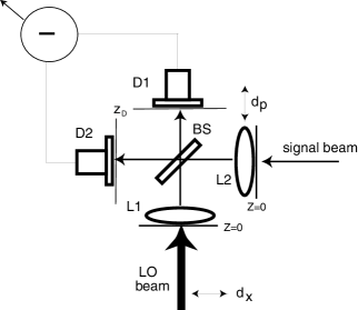
Figure 1: A balanced heterodyne optical imaging scheme.

Since tomography methods developed for spatial properties of photon wave function can be applied to classical field (coherent state with large mean photon number), we use electric field notation $\mathcal{E}(x)$ to represent the wave field $\psi(x)$ in the following Sections.

We use a balanced heterodyne detection scheme as shown in Fig. 1. The beat amplitude $V_{B}$ is determined by the spatial overlap of the local oscillator $(LO)$ and signal $(S)$ fields in the plane of the detector at $Z=Z_{D}$ as,

$$V_{B}=\int dx^{\prime}\mathcal{E}^{*}_{LO}(x^{\prime},z_{D})\mathcal{E}_{S}(x^{\prime},z_{D})$$ (18)

where $x^{\prime}$ denotes the transverse position in the detector plane. When the LO beam is moved by a distance $d_{x}$, the $V_{B}$ becomes,

$$V_{B}(d_{x})=\int dx^{\prime}\mathcal{E}^{*}_{LO}(x^{\prime}-d_{x},z_{D})\mathcal{E}_{S}(x^{\prime},z_{D}).$$ (19)

The fields in the detector plane are related to the fields in the source planes $(z=0)$ of lenses L1 and L2, which have equal focal lengths f = 6 cm. The LO and signal fields at $z=0$ after the lenses, L1 and L2, are given by

$$\mathcal{E}^{\prime}_{LO}(x_{1}-d_{x},z=0) = \exp[-i\frac{k}{2f}x_{1}^{2}]\mathcal{E}_{LO}(x_{1}-d_{x},z=0)$$

$$\mathcal{E}^{\prime}_{S}(x_{2},z=0) = \exp[-i\frac{k}{2f}x_{2}^{2}]\mathcal{E}_{S}(x_{2},z=0)$$

When the lens L2 is scanned by a distance $d_{p}$, the signal field (LABEL:eq:20) is altered as

$$\mathcal{E}^{\prime}_{S}(x_{2},z=0)=\exp[-i\frac{k}{2f}(x_{2}-d_{p})^{2}]\mathcal{E}_{S}(x_{2},z=0)\\$$

The fields propagating a distance $d=f$ to the planes of the detectors can be obtained by using Fresnel’s diffraction integrals as,

$$\mathcal{E}_{LO}(x^{\prime}-d_{x},z_{D}) = \sqrt{\frac{k}{i2\pi f}}\int dx_{1}\,\exp[i\frac{k}{2f}(x_{1}-x^{\prime})^{2}]$$

$$\times \exp[-i\frac{k}{2f}x_{1}^{2}]\,\mathcal{E}_{LO}(x_{1}-d_{x},z=0)$$

$$\mathcal{E}_{S}(x^{\prime},z_{D}) = \sqrt{\frac{k}{i2\pi f}}\int dx_{2}\,\exp[i\frac{k}{2f}(x_{2}-x^{\prime})^{2}]$$ (21)

$$\times \exp[-i\frac{k}{2f}(x_{2}-d_{p})^{2}]\,\mathcal{E}_{S}(x_{2},z=0)$$

By substituting the above equations into Eq. (19), the quadratic phases in $x^{\prime}$ cancel and the quadratic phases that depend on $x_{1,2}^{2}$ cancel in these expressions because the detector plane is in the focal plane of the lenses, L1 and L2. One obtains

$$V_{B}(d_{x},d_{p}) = \frac{k}{f}\,\exp[i\frac{k}{2f}d_{p}^{2}]\int dx_{2}\,\exp[-i\frac{k}{f}x_{2}d_{p}]\,\mathcal{E}_{S}(x_{2},z=0)$$ (22)

$$\times \int dx_{1}\,\mathcal{E}_{LO}^{*}(x_{1}-d_{x},z=0)\delta(x_{1}-x_{2})$$

Integrating over $x_{1}$ and by replacing $x_{2}$ by $x$ and dropping the term $z=0$, the mean square beat amplitude is then given by

$$|V_{B}(d_{x},d_{p})|^{2}\propto\left|\int dx\,\mathcal{E}_{LO}^{*}(x-d_{x})\mathcal{E}_{S}(x)\,\exp(-ik\frac{d_{p}}{f}x)\right|^{2}\\$$

or

$$|V_{B}(d_{x},d_{p})|^{2} \propto \int dx\,\mathcal{E}_{LO}^{*}(x-d_{x})\mathcal{E}_{S}(x)\,\exp(-ik\frac{d_{p}}{f}x)$$ (23)

$$\times \int dx^{\prime}\,\mathcal{E}_{LO}(x^{\prime}-d_{x})\mathcal{E}_{S}^{*}(x^{\prime})\,\exp(ik\frac{d_{p}}{f}x^{\prime}).$$

This can be rewritten using the variable transformations $x=x_{o}+\eta/2$; $x^{\prime}=x_{o}-\eta/2$ where the Jacobian of this transformation is 1. Then, by using the definition of the Wigner distribution,

$$W(x,p)=\int\frac{d\epsilon}{2\pi}\,\exp(i\epsilon p)\langle\,\mathcal{E}^{*}(x+\epsilon/2)\mathcal{E}(x-\epsilon/2)\rangle$$ (24)

and its inverse transform is given by,

$$\mathcal{E}^{*}(x+\epsilon/2)\mathcal{E}(x-\epsilon/2)=\int dp\,\exp(-i\epsilon p)W(x,p),$$ (25)

the beat signal in Eq. (23) becomes

$$|V_{B}(d_{x},d_{p})|^{2} \propto \int dx_{o}\int d\eta\,\mathcal{E}_{LO}^{*}(x_{o}+\eta/2-d_{x})\mathcal{E}_{LO}(x_{o}-\eta/2-d_{x})$$ (26)

$$\times \int dp\,\exp(-ik\frac{d_{p}}{f}\eta)\,\exp(-i\eta p)W_{S}(x,p).$$

Since the Wigner distribution of the LO field is

$$W_{LO}(x_{\circ}-d_{x},p+k\frac{d_{p}}{f}) = \int\frac{d\eta}{2\pi}\,\exp[-i\eta(p+k\frac{d_{p}}{f})]$$ (27)

$$\times \mathcal{E}_{LO}^{*}(x_{o}+\eta/2-d_{x})\mathcal{E}_{LO}(x_{o}-\eta/2-d_{x})$$

then the LO fields in Eq. (26) can be replaced by the Wigner function in Eq. (27). Finally, the mean square heterodyne beat signal $|V_{B}|^{2}$ can now be written as

$$|V_{B}(d_{x},d_{p})|^{2}\propto\int dxdp\,W_{LO}(x-d_{x},p+\frac{k}{d_{p}})W_{S}(x,p)$$ (28)

where $W_{S}(x,p)$ is the Wigner distribution of the signal field in the plane of L2 (z =0) and $W_{LO}(x,p)$ is the LO Wigner distribution in the plane of L1 (z = 0). We include a detail description of two-window heterodyne measurement of KR distribution as shown in Fig. 2. The variables $d_{x}$ and $d_{p}$ respectively indicate the positions of a mirror M1 and a lens L2 as in Fig. 2. Eq. (28) shows that the mean-square beat signal yields a phase-space contour plot of $W_{S}(x,p)$ with phase space resolution determined by $W_{LO}(x,p)$. By using a two-LO heterodyne detection scheme as discussed below, the $|V_{B}(d_{x},d_{p})|^{2}$ is found to be proportional to $\mathcal{K}^{*}(x,p)$.

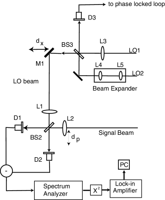
Figure 2: Experimental setup for measuring the KR distribution using two-LO balanced heterodyne detection. $X^{2}$; squarer, D; photodiode detector, BS; beam splitter.

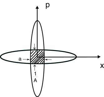
Figure 3: The overlapping area is the position and momentum resolutions of the combined LO beams. The uncertainty is proportional to $\frac{a}{A}$ less than 1.

To obtain independent control of the $x$ and $p$ resolution in heterodyne measurement, we employ a slowly varying LO field containing a focused and a collimated field with a well defined relative phase $\theta$

$$\mathcal{E}_{LO}(x)=\mathcal{E}_{\circ}[\,\exp(-\frac{x^{2}}{2a^{2}})+\alpha\,\exp(-\frac{x^{2}}{2A^{2}})\,\exp(i\theta)]$$ (29)

Here $a$ is chosen to be small compared with the distance scales of interest and $1/A$ is chosen to be small compared with the momentum scales of interest in the signal field. The schematic picture of the overlapping of the LO beam with the spatial width $a$ and another LO beam with the spatial width $A$ is shown in Fig. 3. One can see that the overlapping area is determined by the position and momentum resolutions for the LO fields in Eq. (29). The focussed LO gaussian beam extracts the position information of the signal field and the collimated LO gaussian beam extracts momentum information of the signal field. The Wigner function for the LO field is obtained by substituting Eq. (29) into Eq. (24). We take $A^{2}$$\gg$$a^{2}$. In this case the phase-($\theta$-) dependent part of the Wigner function for the LO takes the form

$$W_{LO}(x,p) \propto exp(-\frac{2x^{2}}{A^{2}}-2a^{2}p^{2})\cos(2xp+\theta)$$ (30)

$$\simeq \cos(2xp+\theta),$$

where the last form assumes that the range of the momentum and position integration in relation (28) is limited by the signal field.

The measurement of phase space distributions is accomplished by translation of optical elements. These elements are all mounted on translation stages driven by computer controlled linear actuators. The system scans the LO position over a distance $d_{x}$ = $\pm 1$ cm by translating mirror M1 in the LO path. The LO momentum is scanned over $\pm 0.3\,k$, where $k=2\pi/\lambda$ is an optical wave vector, by translation of the signal-beam input lens L2 (focal length $f$ = 6 cm) by a distance $d_{p}$.

In the experiments, as illustrated in Fig. 2, the LO beam is obtained by combination of two fields that differ in frequency by 5 kHz, so that $\theta$ =$(2\pi\times 5kHz)t$. Lens L3 focuses beam LO1 to a waist of width $a$, and lenses L4 and L5 expand beam LO2 to width $A$. We combine these two components at beam splitter BS3 to obtain an LO field of the form given in Eq. (29). We monitor one output of the beam splitter with detector $D_{3}$ to phase lock the 5 kHz beat signal to the reference channel of the lock-in amplifier. Each component of the LO beam is shaped so that it is at a beam waist at the input plane of the heterodyne imaging system (lens L1). The focussed gaussian LO beam is frequency shifted at 110 MHz and the collimated gaussian LO beam is frequency shifted at 110 MHz plus 5 kHz. These two LO beams are overlapped with each other and phase locked at 5 kHz. The signal beam is frequency shifted at 120 MHz. Two imaging lenses L1 and L2 are used to overlap the dual LO beam with the signal beam at two detectors. The interference beat signal between the signal beam and the dual LO beam is obtained at detectors 1 and 2 and consists of 10 MHz and 10 MHz plus 5 kHz components. These signals are sent to a spectrum analyzer. The spectrum analyzer bandwidth, 100 kHz, is chosen to be large compared with 5 kHz difference frequency. The output of the analyzer is then squared by using an analog multiplier. The mean square signal has components at 5 kHz. A lock-in amplifier is used to measure the in- and out-of phase components of the multiplier output at 5 kHz. The lock-in outputs for in- and out-of-phase quadratures then directly determine the real and the imaginary parts of the $\mathcal{K}^{*}(x,p)$ function

$$|V_{B}(d_{x},d_{p})|^{2}=\mathcal{K}^{*}(x_{\circ},p_{\circ}) = \int\frac{dx^{\prime}dp^{\prime}}{\pi}\,\exp[2i(x^{\prime}-x_{\circ})\times(p^{\prime}-p_{\circ})]W_{S}(x^{\prime},p^{\prime})$$ (31)

$$= \langle\mathcal{E}^{*}(x_{\circ})\mathcal{E}(p_{\circ})\rangle\,\exp(ix_{\circ}p_{\circ})=S_{R}+iS_{I},$$

where the $W_{LO}(x,p)$ in Eq. (30) is replaced by $e^{i(2xp+\theta)}$ in Eq. (28) yielding the in-phase and out-of-phase contributions from $\theta$. Here $x_{\circ}$ = $d_{x}$ is the center position of the LO fields and $p_{\circ}$ = $-kd_{p}/f$ is the center momentum. The $S_{R}$ and $S_{I}$ components are related to heterodyne beat signal of $E^{*}_{LO1}E_{S}$ and $E^{*}_{LO2}E_{S}$ or intensity correlation of $E^{*}_{LO1}E_{S}$ and $E^{*}_{LO2}E_{S}$. In the balanced heterodyne detection, the output voltage $V_{B}(t)$=$V_{1}(t)-V_{2}(t)$ before being fed into the spectrum analyzer is given by,

$$V_{B}(t)=2E_{S}^{*}E_{LO1}e^{-i(\Omega_{LO1}-\Omega_{S})t}+2E_{S}^{*}E_{LO2}e^{-i(\Omega_{LO2}-\Omega_{S})t}+cc$$ (32)

In spectrum analyzer, the power spectrum of the $V_{B}$ is measured as

$$|V_{B}(\Omega)|^{2}=\int_{-\infty}^{\infty}\frac{d\tau}{2\pi}\,e^{i\Omega\tau}\,\langle V_{B}(t)V_{B}(t+\tau)\rangle.$$ (33)

As mentioned previously, it is squared by using a squarer to recover the beat signal $|V_{B}(\Omega)|^{2}$. From Eq. (33), the power spectrum can be calculated by keeping the slowly varying term $(\Omega_{LO1}-\Omega_{LO2})$ in time $t$ and other terms that depend on $\tau$, that is,

$$\langle V_{B}(t)V_{B}(t+\tau)\rangle = \frac{1}{T}\int_{-T/2}^{T/2}dt\,V_{B}(t)V_{B}(t+\tau)$$

$$\propto E_{S}^{*}E_{LO1}E_{S}E_{LO1}^{*}e^{-i(\Omega_{S}-\Omega_{LO1})\tau}+E_{S}^{*}E_{LO2}E_{S}E_{LO2}^{*}e^{-i(\Omega_{S}-\Omega_{LO2})\tau}$$

$$+ E_{S}^{*}E_{LO1}E_{S}E_{LO2}^{*}e^{-i(\Omega_{LO1}-\Omega_{LO2})t}e^{-i(\Omega_{S}-\Omega_{LO2})\tau}$$

$$+ E_{S}^{*}E_{LO2}E_{S}E_{LO1}^{*}e^{i(\Omega_{LO1}-\Omega_{LO2})t}e^{-i(\Omega_{S}-\Omega_{LO1})\tau}$$

$$+ (\textrm{: the negative frequency contributions from the above terms:})$$

Here, $\Omega_{S}$=120 MHz, $\Omega_{LO1}$=110 MHz + 5 kHz and $\Omega_{LO2}$=110 MHz. Now, by substituting Eq. (LABEL:eq:33) into Eq. (33) to obtain the power spectrum for the beat $V_{B}$ and setting the analyzer at 10 MHz with the bandwidth of 100 kHz, the $|V_{\circ}(t)|^{2}$ at 5 kHz after the recovery by the squarer is

$$|V_{\circ}(t)|^{2}\propto E_{S}^{*}E_{LO1}E_{S}E_{LO2}^{*}e^{-i(\Omega_{LO1}-\Omega_{LO2})t}+cc$$ (35)

Here $\Omega_{LO1}-\Omega_{LO2}$ = 5 kHz. The in-phase and out-of-phase components of the $|V_{\circ}(t)|^{2}$ at 5 kHz correspond to $S_{R}$ and $S_{I}$ in Eq. (31). Note that $E_{S}^{*}E_{LO1}$ is integrated over the transverse plane as is $E_{S}E^{*}_{LO2}$. It is worth noting that the component $E_{S}^{*}E_{LO1}$ of Eq. (35) is corresponding to the measurement of the position distribution in $K^{*}(x_{\circ},p_{\circ})$ of Eq. (31) by the tightly focussed LO1 beam. Similarly, the component $E_{S}E_{LO2}^{*}$ of Eq. (35) indicates the measurement of the momentum distribution in $K^{*}(x_{\circ},p_{\circ})$ of Eq. (31) by the collimated LO2 beam.

As the position of mirror M1 is scanned a distance $d_{x}$, the optical path lengths of the LO fields change. For the current experiments, the HeNe laser is a source, the change in path lengths is small compared with the Rayleigh length and the coherence length of the beams, so translating M1 simply changes the center position of the LO fields.

IV Results

IV.1 Measurement of an Optical Gaussian beam

IV.1.1 Gaussian Beam

As an initial demonstration of the capability of this system, we measure the $\mathcal{K}^{*}(x,p)$ function for an ordinary gaussian beam. A one dimensional wave field for an Gaussian beam of $TEM_{00}$ and radii of curvature, R, is given by,

$$\mathcal{E}(x) \propto \exp({-\frac{x^{2}}{2\sigma^{2}}+i\frac{kx^{2}}{2R}})$$ (36)

$$\propto \mathcal{A}+i\mathcal{B}$$

where the x is the transverse position and $\sigma$ is the waist of signal beam. The Fourier transform of $\mathcal{E}(x)$ is,

$$\mathcal{E}(p) \propto \exp({-\frac{p^{2}}{8\sigma^{2}(\frac{1}{2\sigma^{2}})^{2}+(\frac{k}{2R})^{2}}}{-i\frac{kp^{2}}{8R(\frac{1}{2\sigma^{2}})^{2}+(\frac{k}{2R})^{2}}})$$ (37)

$$\propto \mathcal{C}+i\mathcal{D}$$

The complex conjugated KR distribution for this wave field can be written as,

$$\mathcal{K}^{*}(x,p) = (\mathcal{AC+BD})\cos(xp)+(\mathcal{BC-AD})\sin(xp)$$ (38)

$$+ i((\mathcal{AD-BC})\cos(xp)+(\mathcal{AC-BD})sin(xp))$$

The characteristic function, $\mathcal{M_{KR}}(x,p)$, is obtained from Eq. (11), where the characteristic function for Wigner function for this wave field is given by,

$$\mathcal{M_{W}}(x^{\prime},p^{\prime}) = \int\mathcal{E}^{*}(\eta-\frac{x^{\prime}}{2})\mathcal{E}(\eta+\frac{x^{\prime}}{2})e^{ip^{\prime}\eta}d\eta$$ (39)

$$= \int\mathcal{E}^{*}(\eta+\frac{p^{\prime}}{2})\mathcal{E}(\eta-\frac{p^{\prime}}{2})e^{ix^{\prime}\eta}d\eta$$

$$= \exp(-\frac{x^{\prime}}{4\sigma^{2}}-\frac{\sigma^{2}}{4}(\frac{kx^{\prime}}{R}+p^{\prime})^{2})$$

Then, the Wigner, P- and Q-distributions are obtained from Eq. (14), Eq. (16) and Eq. (17), respectively. The Wigner function for the wave field is given by,

$$W(x,p)=\frac{1}{\pi}\exp(-\frac{x^{2}}{\sigma^{2}}-\sigma^{2}(\frac{kx}{R}+p)^{2})$$ (40)

The P- and Q-distributions for the wave field are given in the integral form as,

$$P(x,p) = \int\exp(-\frac{\sigma^{2}k^{2}x^{\prime 2}}{4R^{2}}-\frac{\sigma^{2}kx^{\prime}p^{\prime}}{2R})exp(-ixp^{\prime}-ipx^{\prime})dx^{\prime}dp^{\prime}$$

$$Q(x,p) = \int\exp(-\frac{x^{\prime 2}}{2\sigma^{2}}-\frac{\sigma^{2}p^{\prime 2}}{2}-\frac{\sigma^{2}k^{2}x^{\prime 2}}{4R^{2}}-\frac{\sigma^{2}kx^{\prime}p^{\prime}}{2R})\exp(-ixp^{\prime}-ipx^{\prime})dx^{\prime}dp^{\prime}$$

For simplicity, the signal Gaussian beam is shaped by a telescope so that its waist coincides with input plane L2 of the heterodyne imaging system. For a gaussian beam at its waist, $R=\infty$, Eq. (38) gives the complex conjugated KR distribution as,

$$\mathcal{K}^{*}(x,p)=\mathcal{AC}\cos(xp)+i\mathcal{AC}\sin(xp)$$ (42)

where $\mathcal{A}=\exp(-\frac{x^{2}}{2\sigma^{2}})$, $\mathcal{C}=\exp(-\frac{p^{2}\sigma^{2}}{2})$, and $\sigma$=0.85 mm is the $1/e$-intensity width. The $\mathcal{K}^{*}(x,p)$ function for the signal field is measured by use of the dual LO beam of the form given by Eq. (29) with $a$ =81 $\mu$m, $A$ = 2.6 mm, and $\alpha$ =1. The measurement result for a gaussian beam is shown in Fig. 4. The top row is our experimental results and the bottom row is a theoretical prediction obtained by using Eq. (42). The real and the imaginary parts of the detected signal, Eq. (31), are shown in Fig. 4(a) and (b). Our observation is similar to the theoretical prediction by Wodkiewicz wodkiewicz03b for a coherent state.

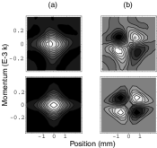
Figure 4: The Wigner function for a gaussian beam. Top row is experimental results and bottom row is theoretical prediction for a gaussian beam. (a) is in-phase component of $\mathcal{K}^{*}(x_{\circ},p_{\circ})$ and (b) is out-of-phase component of $\mathcal{K}^{*}(x_{\circ},p_{\circ})$

.

Position (momentum) distributions of this field can be obtained through the summation of momentum (position) coordinate of real and the imaginary parts of the measured $\mathcal{K}^{*}(x,p)$. The position and momentum distributions are shown in Fig. 5 and Fig. 6, respectively. The imaginary part of position and momentum distribution are around zero as theoretically predicted by $\int\mathcal{K}^{*}(x,p)dp=|\mathcal{E}(x)|^{2}$ and $\int\mathcal{K}^{*}(x,p)dx=|\mathcal{E}(p)|^{2}$, respectively, which are the real physical quantities (no complex values). From here, the position and momentum distributions are fitted with Gaussian function. We obtain the beam waist of $\sigma$ = 0.86 from position distribution and $\sigma$=0.87 from momentum distribution. Both results are in excellent agreement with the measured width $\sigma$=0.85 mm obtained by use of a diode array, demonstrating that high position and momentum resolution can be jointly obtained.

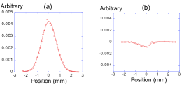
Figure 5: (a) Real part and (b) imaginary part of position distribution of a Gaussian field. Imaginary part is around zero.

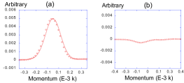
Figure 6: a) Real part and (b) imaginary part of momentum distribution of a Gaussian field. Imaginary part is around zero.

Wigner distribution is obtained by using simple linear transformation as discussion in Eq. (14) or Eq. (15) as shown in Fig. 7(a). We $\chi^{2}$ fit the width of the measured in-phase signal in position for $p$ = 0 to obtain a spatial width $\sigma$ =0.87 mm, whereas the corresponding momentum distribution for $x$ = 0 yields $\sigma$ =0.83 mm.

The characteristic function $\mathcal{M}_{KR}(x^{\prime},p^{\prime})$ is obtained by using numerical integration of the measured $\mathcal{K}^{*}(x.p)$ as in Eq. (13). The P- and Q- distributions for this signal gaussian beam are then obtained through the Eq. (16) and Eq. (17), as shown in Fig. 7(b) and Fig. 7 (c), respectively. The P-distribution has a narrower peak in phase-space compared to other distributions. This is predicted for the signal beam with $R=\infty$ in P-distribution of Eq. (LABEL:eq:40), which we should have $\delta(x)\delta(p)$ in phase-space. The Q-distribution has a broad peak in phase-space compared to other distributions. The Q-distribution for this signal beam can be evaluated from Eq. (LABEL:eq:40) with $R=\infty$, as given by,

$$Q(x,p)\propto\exp(-\frac{p^{2}\sigma^{2}}{2}-\frac{x^{2}}{2\sigma^{2}}).$$ (43)

The position width of the Q-distribution at p=0 is about $\sqrt{2}$ larger than the position width of Wigner distribution at p=0 as from Eq. (40). Hence, the beam waist for the signal beam obtained from the Q-distribution is $\sqrt{2}$ larger than the exact value.

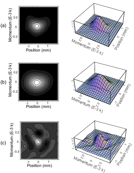
Figure 7: (a) The reconstructed Wigner distribution, (b) Husimi or Q-distribution, and (c) Glauber Sudarshan P-distribution for an optical Gaussian beam. 2D-plot(left);3D-plot(right).

IV.1.2 Measurement of superposition of two slightly displaced coherent beams

As a fundamental feature in the process of quantum measurement, we cannot observe physical properties of a quantum objects directly because the overall backaction of any observation cannot be made less than Planck’s constant h. Instead, we observe the wave or the particle aspects of the physical objects. The $\mathcal{K}^{*}(x,p)$ distribution for a coherent field is more likely representing particle picture of the field because it contains local information of the coherent field. While the Wigner function is more likely representing wave behavior of the field because it exhibits phase-space interference. Based on these properties, the $\mathcal{K}^{*}(x,p)$ and Wigner distributions are very useful to characterize a wave field or an physical object through phase-space imaging in many applications such as quantum imaging, metrology, and biomedical imaging. To illustrate the particle picture of $\mathcal{K}^{*}(x,p)$ and the wave picture of Wigner function, we use the same signal gaussian beam obscured by a wire with diameter of 1 mm. Then, the electric field $\mathcal{E}_{s}(x)$ as a function of position is shown in Fig. 8. It didn’t involve convolution integration because the wire is placed close to the imaging lens L2. It shows the superposition of two slightly displaced coherent beams. It is analogous to a Schrödinger cat state. In this case, the slowly varying field is gaussian as before but multiplied by a slit function that sets the field equal to zero for $|x|\leq 0.5$ mm. Fig. 9 shows contour plots of the real and the imaginary parts of the detected signal of $\mathcal{K}^{*}(x,p)$.

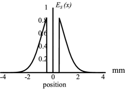
Figure 8: The wave field $\mathcal{E}(x)$ of a Gaussian beam obscured by a wire.

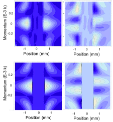
Figure 9: Top row shows experimental results and bottom row shows theoretical predictions for a gaussian beam blocked by a wire. (a) in-phase component of the $\mathcal{K}^{*}(x_{\circ},p_{\circ})$ and (b) out-of-phase component of the $\mathcal{K}^{*}(x_{\circ},p_{\circ})$.

The top row is our experimental results. The bottom row is theoretical prediction. The theoretical plots are first obtained by numerically generating the signal function $\mathcal{E}_{S}(x)$ and its Fourier transform $\mathcal{E}_{S}(p)$. The real and imaginary parts of $\mathcal{K}^{*}(x,p)$ in Eq. (10) are then theoretically plotted. The real and imaginary parts are not showing phase-space interferences of two slightly displaced coherent beams. These plots show local information of the signal field, i.e., zero(nonzero) field is corresponding to zero(nonzero) $\mathcal{K}^{*}(x,p)$ phase-space distribution. This locality property exhibits particle picture if an atomic wave function/single photon function is used. The position and momentum distributions are then retrieved $\int\mathcal{K}^{*}(x,p)dp$ and $\int\mathcal{K}^{*}(x,p)dx$ as shown in Fig. 10 and Fig. 11, respectively. The momentum distribution contains the interference features of two spatially separated wave packets of $\mathcal{E}_{S}(x)$ as shown in Fig. 11. The imaginary part of these distributions are around zero as expected.

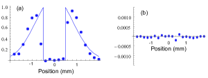
Figure 10: (a) The real part, (b) the imaginary part of the position distribution of a wire function obtained by integrating the measured KR distribution over momentum. Imaginary part is around zero.

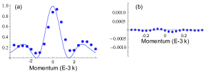
Figure 11: (a) The real part, (b) the imaginary part of the momentum distribution of a wire function obtained by integrating the measured KR distribution over position. Imaginary part is around zero.

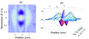
Figure 12: The reconstructed Wigner distribution for a wire function (a) two-, (c) three- dimensional plot.

The Wigner function as shown in Fig. 12 is reconstructed by using the linear transformation of the measured $\mathcal{K}^{*}(x,p)$. The coherence between these two wave packets in the signal field leads to an phase-space interference pattern in the momentum distribution. The signature of this coherence in the Wigner distribution is the oscillating positive and negative values between the main lobes. An interesting feature of this Wigner distribution is the oscillation in momentum at the position $x$ =0 of the wire. We observe the negative values which is analogous to quantum interference in phase space. This feature can be seen in Fig. 12, in which the reconstructed Wigner function is shown as a three dimensional plot. The negative values highlight the impossibility of a particle simultaneously having a precise position and momentum. It also makes sure that the sum over momentum along x = 0 in the reconstructed Wigner distribution has zero intensity at the center. The negative and positive parts of the Wigner phase space distribution are important features to obtain full information about the field. Our observation of the negative values of Wigner function for this coherent field did not claim that the negative values exhibited by a quantum field is not a quantum feature. We believe that classical or quantum features of an experiment are based on classical or quantum field involved in the experiment.

From the obtained Wigner function, one can obtain the position and momentum distribution of the $\mathcal{E}_{s}(x)$ by using the formulas $|\mathcal{E}_{S}(p)|^{2}$=$\int_{-\infty}^{\infty}W_{S}(x,p)\,dx$ and $|\mathcal{E}_{S}(x)|^{2}$=$\int_{-\infty}^{\infty}W_{S}(x,p)\,dp$ as shown in Fig. 13(b) and (d) respectively. The resolution of these plots is better than Fig. 10 and Fig. 11 because we numerically generate more data points from the reconstructed Wigner function. The measurements are in agreement with the theoretical predictions as shown in Fig. 13(a) and (c) respectively.

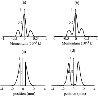
Figure 13: The momentum and position distribution for the Schrödinger cat state. (a) and (c) are theoretical prediction of momentum and position distributions of the cat state. (b) and (d) are the corresponding experimental results of momentum and position distribution of the cat state obtained by integrating the measured Wigner distribution over $p$ and $x$ respectively.

As discussed before, we first obtain the characteristic function $\mathcal{M}_{KR}(x^{\prime},p^{\prime})$ and then the P- and Q- distributions for this signal field. These distributions are plotted in Fig. 14 (a) and (b), respectively. The Q-distribution exhibits the broadening or low resolution of phase-space features compared to Wigner function. While the P-distribution is not a well behaved function for this field as it is expected for P-distribution.

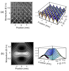
Figure 14: The reconstructed (a) P- and (b) Q-distributions for a slightly displaced coherent beams. 2D-plot(left); 3D-plot(right).

V Discussion and Conclusions

Spatial properties of photon wave mechanics approach smith07 for a single photon have been studied in detail. The approach can be applied to both single photon state and coherent field. As a consequence, the coherent field is the best testing ground for developing tomography method for quantum information processing. In the similar efforts, coherent fields have played an important role in quantum communication and computing such as search algorithm lloyd00 ; spreeuw02 ; spreeuw01 ; kim09 and factorization of numbers schleich08 . Optical wave mechanics implementations kim04 ; kim02 of entanglement and superposition with coherent fields (coherent state with large photon numbers) have been demonstrated. This implementation has been used to study entanglement swapping and tests of non-locality. However, photon wave mechanic approach for two- and multi-photon spatial qubits haven’t been relatively explored. The two-LO technique developed in this paper will provide another tomography tools to explore spatial qubits because it could provide the particle picture through KR distribution and wave picture through Wigner distribution.

We would like to discuss KR and Wigner distribution separately because the particle and wave picture of wave field can provide independent useful information for quantum and coherent information processing including biomedical imaging brezinski08 .

Particle picture or local information of a wave field represented by KR distribution has advantages in positioning or angle (momentum) resolving to extract local activities of an target. The method can directly locate the field or structure of an object without applying any raw data transformation. This will be particularly useful in cell tissue characterization such as prostate cancer cell detection. The KR distribution can be used to study Goos-Hanchen (GH) shifts saleh98 occur in near field optics and photonic waveguide. GH shifts in position and momentum can be used to identify the loss due to photonic crystal waveguide fabrication.

Wave picture or nonlocal information of a wave field is best represented by Wigner function. We observe the non-positive properties of the Wigner function for a superposition of two spatially separated gaussian field $\mathcal{E}(x)$ analogous to a Schrödinger cat state in spatial coordinate. We have demonstrated the similarities in phase space interference between spatial properties of quantum and coherent fields via the measurement of the Wigner function. We also show that an interesting analogy exists between our choice of LO field and that employed in the quantum-teleportation experiment furusawa98 . In the x-p representation, the small and the large beams of our two-LO can be viewed as superposition of the position (in-phase) and the momentum (out-of-phase) squeezed fields. A $\mathcal{E}(x)$ spatial gaussian field of $TEM_{00}$ is the lowest mode and is similar to a coherent state in phase-space picture. Gaussian beams of smaller (larger) size than the lowest mode correspond to position (momentum) squeezed states. The two-LO technique here can only be used if we know the nominal size of the signal beam. The focussed and collimated LO beams must be chosen to achieve sufficient $x-$ and $p-$ resolution for the given signal beam. These are the similar problems encountered in our experiments and in the quantum teleportation experiments which teleport an arbitrary state as a Wigner function via EPR beams furusawa98 .

In a complex multi-particle system or large N-biological system, we believe KR and Wigner distributions are very useful to study the local and nonlocal information of a macroscopic wave field such as the mechanisms of decoherence due to neighbor particles, quantum mapping of N-particle system or semiclassical system, and macroscopic entanglement between two macroscopic mirrors.

In conclusion, we have demonstrated the direct measurement of KR distribution using two-LO balanced heterodyne detection technique. The characteristic function of KR is related to Wigner, P and Q- distributions. Then, the Wigner, P and Q- distribution are plotted by using raw data from the KR distribution. The physical properties of a wave field such as local and nonlocal phase space information are illustrated through KR and Wigner functions, respectively. This two-LO technique can be used in information processing including quantum information for quantum mapping and optical imaging for biomedical applications.

References

- (1) K. F. Lee, F. Reil, S. Bali, A. Wax, and J. E. Thomas, Opt. Lett. 24, 1370-2 (1999).
- (2) A. Wax, and J. E. Thomas, Opt. Lett. 21,1427(1996).
- (3) A. Wax, S. Bali, and J. E. Thomas, Phys. Rev. Lett.85, 66(2001).
- (4) F. Reil, and J. E. Thomas, Phys. Rev. Lett. 95, 143903(2005).
- (5) C. Iaconis, and I. A. Walmsley, Opt. Lett. 21, 1783(1996).
- (6) C. C. Cheng, and M. G. Raymer, Phys. Rev. Lett. 82, 4807 (1999).
- (7) Smith, B. J., B. Killett, M. G. Raymer, I. A. Walmsley, and K. Banaszek, Opt. Lett. 30, 3365 (2005).
- (8) Mukamel, E., K. Banaszek, I. A. Walmsley, and C. Dorrer, Opt. Lett. 28, 1317(2003).
- (9) J. G. Kirkwood, Phys. Rev. 44, 31-37 (1933).
- (10) E. P. Wigner, Phys. Rev. 40, 749-759(1932).
- (11) A. N. Rihaczek, IEEE Trans. Inf. Theory. 14, 369 374 (1968).
- (12) S. John, G. Pang, and Y. Yang, J. Biomed. Opt. 1, 180 (1996).
- (13) M. J. Bastiaans, Opt. Commun. 25, 26 (1978).
- (14) M. J. Bastiaans, The Wigner Distribution-Theory and Applications in Signal Processing, W. Mecklenbrauker and F. Hlawatsch, eds. (Elsevier), 375-426 (1997).
- (15) K. Vogel, and H. Risken, Phys. Rev. A 40, 2847 (1989).
- (16) D. T. Smithey, M. Beck, M. G. Raymer, and A. Faridani, Phys. Rev. Lett. 70, 1244 (1993).
- (17) A. I. Lvovsky and M. G. Raymer, Rev. Mod. Phys. 81, 299 (2009).
- (18) M. G. Raymer, M. Beck, and D.F. McAlister, Phys. Rev. Lett. 72, 1137 (1994).
- (19) D.F. McAlister, M. Beck, L. Clarke, A. Meyer, and M.G. Raymer, Opt. Lett. 20, 1181 (1995).
- (20) M. Beck, M.G. Raymer, I.A. Walmsley and V. Wong, Opt. Lett. 18, 2041 (1993).
- (21) Mikhail I. Kolobov, Quantum Imaging, Springer; 1 edition (2006).
- (22) M. I. Kolobov, Rev. Mod. Phys. 71, 1539-1589 (1999).
- (23) Kolobov, M. I., and I. V. Sokolov, Sov. Phys. JETP 63, 1105 (1986).
- (24) Kolobov, M. I., and I. V. Sokolov, Sov. Phys. JETP 69, 1097 (1989).
- (25) Kolobov, M. I., and I. V. Sokolov, Phys. Lett. A 140, 101(1989).
- (26) Kolobov, M. I., and I. V. Sokolov, Opt. Spectrosc. 66, 440 (1989).
- (27) Kolobov, M. I., and I. V. Sokolov, Europhys. Lett. 15, 271(1991).
- (28) K. E. Cahil and R.J.Glauber, Phys. Rev. 177, 1882-1902 (1969).
- (29) E. C. G. Sudarshan, Phys. Rev. Lett. 10, 277 279 (1963).
- (30) K. Husimi, Proc. Phys. Math. Soc. Jpn. 22, 264 314 (1940).
- (31) Smith, B. J., and M. G. Raymer, New J. Phys. 9, 414 (2007).
- (32) L. Praxmeyer and K. W dkiewicz, Phys. Rev. A 67, 054502 (2003).
- (33) L. Praxmeyer and K. W dkiewicz, Opt. Commun. 223, 349 365 (2003).
- (34) J. P. Dahl, H. Mack, A. Wolf, and W. P. Schleich, Phys. Rev. A 74, 042323(2006).
- (35) K. Banaszek and K. Wodkiewicz, Phys. Rev. Lett. 82, 2009-2013(1999).
- (36) W. P. Schleich, Quantum Optics in Phase Space (Wiley-VCH, 2001).
- (37) F. Toscano, D.A.R. Dalvit, L. Davidovich, and W. H. Zurek, Phys. Rev. A 73, 023803 (2006).
- (38) W. H. Zurek, Nature 412, 712 (2001).
- (39) M. E. Brezinski and B. Liu, Phys. Rev. A 78, 063824(2008).
- (40) R. Loudon, The Quantum Theory of Light, Oxford University Press, USA; 3 edition (2000)
- (41) K. Wagner, J. Janousek, V. Delaubert, H. Zou, C. Hard, N. Treps, J. F. Morizur, . P. K. Lam, and H. A. Bachor, Science 321, 541(2008).
- (42) J. P. Paz, A. J. Roncaglia, and M. Saraceno, Phys. Rev. A 69, 032312 (2004).
- (43) C. Miquel, J. P. Paz, and M. Saraceno, Phys. Rev. A 65, 062309 (2002).
- (44) Seth Lloyd, Phys. Rev. A 61, 010301 (2000).
- (45) N. Bhattacharya, H. B. van Linden, Van den Heuvell, and R. J. Spreeuw, Phys. Rev. Lett. 88, 137901 (2002).
- (46) R. J. Spreeuw, Phys. Rev. A. 63, 062302 (2001).
- (47) K. F. Lee, Opt. Lett. 34, 1099 (2009).
- (48) Damien Bigourd, B. Chatel, W. P. Schleich, and B. Girard, Phys. Rev. Lett. 100, 030202 (2008).
- (49) K. F. Lee and J. E. Thomas, Phys. Rev. A. 69, 052311 (2004).
- (50) K. F. Lee and J. E. Thomas, Phys. Rev. Lett., 88, 097902 (2002).
- (51) Bradley M. Jost, Abdul-Azeez R. Al-Rashed, and Bahaa E. A. Saleh, Phys. Rev. Lett. 81, 2233 (1998).
- (52) A. Furusawa, J. L. Sorensen, S. L. Braunstein, C. A. Fuchs, H. J. Kimble, and E. S. Polzik, Science 282, 706-709 (1998).