Gravitational energy as dark energy: Average observational quantities∗
Abstract
In the timescape scenario cosmic acceleration is understand as an apparent effect, due to gravitational energy gradients that grow when spatial curvature gradients become significant with the nonlinear growth of cosmic structure. This affects the calibratation of local geometry to the solutions of the volume–average evolution equations corrected by backreaction. In this paper I discuss recent work on defining observational tests for average geometric quantities which can distinguish the timescape model from a cosmological constant or other models of dark energy.
Keywords:
dark energy, theoretical cosmology, observational cosmology:
98.80.-k 98.80.Es 95.36.+x 98.80.Jk1 Introduction
I will discuss some recent results on observational tests obs of a model cosmology, which represents a new approach to understanding the phenomenology of dark energy as a consequence of the effect of the growth of inhomogeneous structures. The basic idea, outlined in a nontechnical manner in ref. dark07 , is that as inhomogeneities grow one must consider not only their backreaction on average cosmic evolution – as discussed by other contributors to this volume – but also the variance in the geometry as it affects the calibration of clocks and rods of ideal observers. Dark energy is then effectively realised as a misidentification of gravitational energy gradients.
Although the standard Lambda Cold Dark Matter (CDM) model provides a good fit to many tests, there are tensions between some tests, and also a number of puzzles and anomalies. Furthermore, at the present epoch the observed universe is only statistically homogeneous once one samples on scales of 150–300 Mpc. Below such scales it displays a web–like structure, dominated in volume by voids. Some 40%–50% of the volume of the present epoch universe is in voids with on scales of 30 Mpc HV , where is the dimensionless parameter related to the Hubble constant by . Once one also accounts for numerous minivoids, and perhaps also a few larger voids, then it appears that the present epoch universe is void-dominated. Clusters of galaxies are spread in sheets that surround these voids, and in thin filaments that thread them.
One particular consequence of a matter distribution that is only statistically homogeneous, rather than exactly homogeneous, is that when the Einstein equations are averaged they do not evolve as a smooth Friedmann–Lemaître–Robertson–Walker (FLRW) geometry. Instead the Friedmann equations are supplemented by additional backreaction terms buch00 . Whether or not one can fully explain the expansion history of the universe as a consequence of the growth of inhomogeneities and backreaction, without a fluid–like dark energy, is the subject of ongoing debate buch08 .
Elsewhere in this volume, Peebles Peebles provides some of the arguments that have been presented against backreaction. His line of reasoning is that of a plausibility argument: if we assume a FLRW geometry with small perturbations, and estimate the magnitude of the perturbations from the typical rotational and peculiar velocities of galaxies, then the corrections of inhomogeneities are consistently small. This would be a powerful argument, were it not for the fact that at the present epoch galaxies are not homogeneously distributed. The Hubble Deep Field reveals that galaxies were close to being homogeneous distributed at early epochs, but following the growth voids at redshifts that is no longer the case today. Therefore galaxies cannot be consistently treated as randomly distributed gas particles on the 30 Mpc scales HV that dominate present cosmic structure below the scale of statistical homogeneity.
Over the past few years I have developed a new physical interpretation of cosmological solutions within the Buchert averaging scheme clocks ; sol ; equiv . I start by noting that in the presence of strong spatial curvature gradients, not only should the average evolution equations be replaced by equations with terms involving backreaction, but the physical interpretation of average quantities must also account for the differences between the local geometry and the average geometry. In other words, geometric variance can be just as important as geometric averaging when it comes to the physical interpretation of the expansion history of the universe.
I proceed from the fact that structure formation provides a natural division of scales in the observed universe. As observers in galaxies, we and the objects we observe in other galaxies are necessarily in bound structures, which formed from density perturbations that were greater than critical density. If we consider the evidence of the large scale structure surveys on the other hand, then the average location by volume in the present epoch universe is in a void, which is negatively curved. We can expect systematic differences in spatial curvature between the average mass environment, in bound structures, and the volume-average environment, in voids.
Spatial curvature gradients will in general give rise to gravitational energy gradients. Physically this can be understood in terms of a relative deceleration of expanding regions of different densities. Those in the denser region decelerate more and age less. Since we are dealing with weak fields the relative deceleration of the background is small. Nonetheless even if the relative deceleration is typically of order ms-2, cumulatively over the age of the universe it leads to significant clock rate variances equiv . I proceed from an ansatz that the variance in gravitational energy is correlated with the average spatial curvature in such a way as to implicitly solve the Sandage–de Vaucouleurs paradox that a statistically quiet, broadly isotropic, Hubble flow is observed deep below the scale of statistical homogeneity. In particular, galaxy peculiar velocities have a small magnitude with respect to a local regional volume expansion. Expanding regions of different densities are patched together so that the regionally measured expansion remains uniform. Such regional expansion refers to the variation of the regional proper length, , with respect to proper time of isotropic observers (those who see an isotropic mean CMB). Although voids open up faster, so that their proper volume increases more quickly, on account of gravitational energy gradients the local clocks will also tick faster in a compensating manner.
Details of the fitting of local observables to average quantities for solutions to the Buchert formalism are described in detail in refs. clocks ; sol . Negatively curved voids, and spatially flat expanding wall regions within which galaxy clusters are located, are combined in a Buchert average
| (1) |
where is the wall volume fraction and is the void volume fraction, being the present horizon volume, and , and initial values at last scattering. The time parameter, , is the volume–average time parameter of the Buchert formalism, but does not coincide with that of local measurements in galaxies. In trying to fit a FLRW solution to the universe we attempt to match our local spatially flat wall geometry
| (2) |
to the whole universe, when in reality the rods and clocks of ideal isotropic observers vary with gradients in spatial curvature and gravitational energy. By conformally matching radial null geodesics with those of the Buchert average solutions, the geometry (2) may be extended to cosmological scales as the dressed geometry
| (3) |
where , is the relative lapse function between wall clocks and volume–average ones, , and , where is given by integrating along null geodesics.
In addition to the bare cosmological parameters which describe the Buchert equations, one obtains dressed parameters relative to the geometry (3). For example, the dressed matter density parameter is , where is the bare matter density parameter. The dressed parameters take numerical values close to the ones inferred in standard FLRW models.
2 Apparent acceleration and Hubble flow variance
The gradient in gravitational energy and cumulative differences of clock rates between wall observers and volume average ones has important physical consequences. Using the exact solution obtained in ref. sol , one finds that a volume average observer would infer an effective deceleration parameter , which is always positive since there is no global acceleration. However, a wall observer infers a dressed deceleration parameter
| (4) |
where the dressed Hubble parameter is given by
| (5) |
At early times when the dressed and bare deceleration parameter both take the Einstein–de Sitter value . However, unlike the bare parameter which monotonically decreases to zero, the dressed parameter becomes negative when and at late times. For the best-fit parameters LNW the apparent acceleration begins at a redshift .
Cosmic acceleration is thus revealed as an apparent effect which arises due to the cumulative clock rate variance of wall observers relative to volume–average observers. It becomes significant only when the voids begin to dominate the universe by volume. Since the epoch of onset of apparent acceleration is directly related to the void fraction, , this solves one cosmic coincidence problem.
In addition to apparent cosmic acceleration, a second important apparent effect will arise if one considers scales below that of statistical homogeneity. By any one set of clocks it will appear that voids expand faster than wall regions. Thus a wall observer will see galaxies on the far side of a dominant void of diameter Mpc recede at a rate greater than the dressed global average , while galaxies within an ideal wall will recede at a rate less than . Since the uniform bare rate would also be the local value within an ideal wall, eq. (5) gives a measure of the variance in the apparent Hubble flow. The best-fit parameters LNW give a dressed Hubble constant , and a bare Hubble constant . The present epoch variance is 17–22%.
Since voids dominate the universe by volume at the present epoch, any observer in a galaxy in a typical wall region will measure locally higher values of the Hubble constant, with peak values of order at the Mpc scale of the dominant voids. Over larger distances, as the line of sight intersects more walls as well as voids, a radial spherically symmetric average will give an average Hubble constant whose value decreases from the maximum at the Mpc scale to the dressed global average value, as the scale of homogeneity is approached at roughly the baryon acoustic oscillation (BAO) scale of Mpc. This predicted effect could account for the Hubble bubble JRK and more detailed studies of the scale dependence of the local Hubble flow LS .
In fact, the variance of the local Hubble flow below the scale of homogeneity should correlate strongly to observed structures in a manner which has no equivalent prediction in FLRW models.
3 Future observational tests
There are two types of potential cosmological tests that can be developed; those relating to scales below that of statistical homogeneity as discussed above, and those that relate to averages on our past light cone on scales much greater than the scale of statistical homogeneity. The second class of tests includes equivalents to all the standard cosmological tests of the standard FLRW model with Newtonian perturbations. This second class of tests can be further divided into tests which just deal with the bulk cosmological averages (luminosity and angular diameter distances etc), and those that deal with the variance from the growth of structures (late epoch integrated Sachs–Wolfe effect, cosmic shear, redshift space distortions etc). Here I will concentrate solely on the simplest tests which are directly related to luminosity and angular diameter distance measures.
In the timescape cosmology we have an effective dressed luminosity distance
| (6) |
where , and
| (7) |
We can also define an effective angular diameter distance, , and an effective comoving distance, , to a redshift in the standard fashion
| (8) |
A direct method of comparing the distance measures with those of homogeneous models with dark energy, is to observe that for a standard spatially flat cosmology with dark energy obeying an equation of state , the quantity
| (9) |
does not depend on the value of the Hubble constant, , but only directly on . Since the best-fit values of are potentially different for the different scenarios, a comparison of curves as a function of redshift for the timescape model versus the CDM model gives a good indication of where the largest differences can be expected, independently of the value of . Such a comparison is made in Fig. 1.
(a)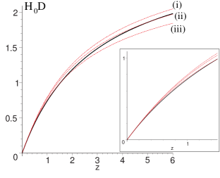 (b)
(b)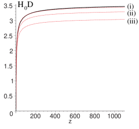
We see that as redshift increases the timescape model interpolates between CDM models with different values of . For redshifts is very close to for the parameter values (model (iii)) which best–fit the Riess07 supernovae (SneIa) data Riess07 only, by our own analysis. For very large redshifts that approach the surface of last scattering, , on the other hand, very closely matches for the parameter values (model (i)) which best–fit WMAP5 only wmap5 . Over redshifts , at which scales independent tests are conceivable, makes a transition over corresponding curves of with intermediate values of . The curve for joint best-fit parameters to SneIa, BAO measurements and WMAP5 wmap5 , is best–matched over the range , for example.
The difference of from any single curve is perhaps most pronounced in the range , which may be an optimal regime to probe in future experiments. Gamma–ray bursters (GRBs) now probe distances to redshifts , and could be very useful. A considerable amount work of work has already been done on Hubble diagrams for GRBs. (See, e.g., GRB .) Much more work is needed to nail down systematic uncertainties, but GRBs may eventually provide a definitive test in future. An analysis of the timescape model Hubble diagram using 69 GRBs has just been performed by Schaefer Schaefer , who finds that it fits the data better than the concordance CDM model, but not yet by a huge margin. As more data is accumulated, it should become possible to distinguish the models if the issues with the standardization of GRBs can be ironed out.
3.1 The effective “equation of state”
It should be noted that the shape of the curves depicted in Fig. 1 represent the observable quantity one is actually measuring when some researchers loosely talk about “measuring the equation of state”. For spatially flat dark energy models, with given by (9), one finds that the function appearing in the fluid equation of state is related to the first and second derivatives of (9) by
| (10) |
where prime denotes a derivative with respect to . Such a relation can be applied to observed distance measurements, regardless of whether the underlying cosmology has dark energy or not. Since it involves first and second derivatives of the observed quantities, it is actually much more difficult to determine observationally than directly fitting .
The equivalent of the “equation of state”, , for the timescape model is plotted in Fig. 2. The fact that is undefined at a particular redshift and changes sign through simply reflects the fact that in (10) we are dividing by a quantity which goes to zero for the timescape model, even though the underlying curve of Fig. 1 is smooth. Since one is not dealing with a dark energy fluid in the present case, simply has no physical meaning. Nonetheless, phenomenologically the results do agree with the usual inferences about for fits of standard dark energy cosmologies to SneIa data. For the canonical model of Fig. 2(a) one finds that the average value of on the range , while the average value of if the range of redshifts is extended to higher values. The “phantom divide” is crossed at for . One recent study ZZ finds mild 95% evidence for an equation of state that crosses the phantom divide from to in the range in accord with the timescape expectation. By contrast, another study SCHMPS at redshifts draws different conclusions about dynamical dark energy, but for the given uncertainties in the data is consistent with Fig. 1(a) as well as with a cosmological constant obs .
The fact that is a different sign to the dark energy case for is another way of viewing our statement above that the redshift range may be optimal for discriminating model differences.
(a) (b)
(b)
3.2 The measure
Further observational diagnostics can be devised if the expansion rate can be observationally determined as a function of redshift. Recently such a determination of at and has been made using redshift space distortions of the BAO scale in the CDM model GCH . This technique is of course model dependent, and the Kaiser effect would have to be re-examined in the timescape model before a direct comparison of observational results could be made. A model–independent measure of , the redshift time drift test, is discussed below.
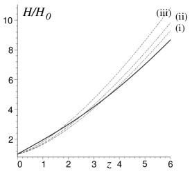
In Fig. 3 we compare for the timescape model to spatially flat CDM models with the same parameters chosen in Fig. 1. The most notable feature is that the slope of is less than in the CDM case, as is to be expected for a model whose (dressed) deceleration parameter varies more slowly than for CDM.
3.3 The measure
Recently a number of authors GCC ; SSS ; ZC have discussed various roughly equivalent diagnostics of dark energy. For example, Sahni, Shafieloo and Starobinsky SSS , have proposed a diagnostic function
| (11) |
on account of the fact that it is equal to the constant present epoch matter density parameter, , at all redshifts for a spatially flat FLRW model with pressureless dust and a cosmological constant. However, it is not constant if the cosmological constant is replaced by other forms of dark energy. For general FLRW models, , which only involves a single derivatives of . Thus the diagnostic (11) is easier to reconstruct observationally than the equation of state parameter, .
(a) (b)
(b)
The quantity is readily calculated for the timescape model, and the result is displayed in Fig. 4. What is striking about Fig. 4, as compared to the curves for quintessence and phantom dark energy models as plotted in ref. SSS , is that the initial value
| (12) |
is substantially larger than in the spatially flat dark energy models. Furthermore, for the timescape model does not asymptote to the dressed density parameter in any redshift range. For quintessence models , while for phantom models , and in both cases as . In the timescape model, for , while for . It thus behaves more like a quintessence model for low , in accordance with Fig. 2. However, the steeper slope and the different large behaviour mean the diagnostic is generally very different to that of typical dark energy models. For large , , if .
Interestingly enough, a recent analysis of SneIa, BAO and CMB data SSS2 for dark energy models with two different empirical fitting functions for gives an intercept which is larger than expected for typical quintessence or phantom energy models, and in the better fit of the two models the intercept (see Fig. 3 of ref. SSS2 ) is close to the value expected for the timescape model, which is tightly constrained to the range if .
3.4 The Alcock–Paczyński test and baryon acoustic oscillations
Some time ago Alcock and Paczyński devised a test AP which relies on comparing the radial and transverse proper length scales of spherical standard volumes comoving with the Hubble flow. This test, which determines the function
| (13) |
was originally conceived to distinguish FLRW models with a cosmological constant from those without a term. The test is free from many evolutionary effects, but relies on one being able to remove systematic distortions due to peculiar velocities.
Current detections of the BAO scale in galaxy clustering statistics bao ; Percival can in fact be viewed as a variant of the Alcock–Paczyński test, as they make use of both the transverse and radial dilations of the fiducial comoving BAO scale to present a measure
| (14) |
(a)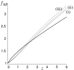 (b)
(b)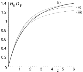
In Fig. 5 the Alcock–Paczyński test function (13) and BAO scale measure (14) of the timescape model are compared to those of the spatially flat CDM model with different values of (,). Over the range of redshifts studied currently with galaxy clustering statistics, the curve distinguishes the timescape model from the CDM models much more strongly than the test function. In particular, the timescape has a distinctly different shape to that of the CDM model, being convex. The primary reason for use of the integral measure (14) has been a lack of data. Future measurements with enough data to separate the radial and angular BAO scales are a potentially powerful way of distinguishing the timescape model from CDM.
Recently Gaztañaga, Cabré and Hui GCH have made the first efforts to separate the radial and angular BAO scales in different redshift slices. Although they have not yet published separate values for the radial and angular scales, their results are interesting when compared to the expectations of the timescape model. Their study yields best-fit values of the present total matter and baryonic matter density parameters, and , which are in tension with WMAP5 parameters fit to the CDM model. In particular, the ratio of non-baryonic cold dark matter to baryonic matter has a best-fit value of 3.7 in the sample, 2.6 in the sample, and 3.6 in the whole sample, as compared to the expected value of 6.1 from WMAP5. The analysis of the 3–point correlation function yields similar conclusions, with a best fit GCCCF , . By comparison, the parameter fit to the timescape model of ref. LNW yields dressed parameters , , and a ratio . Since other forms of dark energy are not generally expected to give rise to a renormalization of the ratio of non-baryonic to baryonic matter, this is encouraging for the timescape model.
3.5 Test of (in)homogeneity
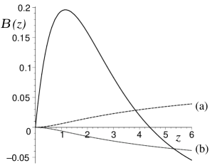
Recently Clarkson, Bassett and Lu CBL have constructed what they call a “test of the Copernican principle” based on the observation that for homogeneous, isotropic models which obey the Friedmann equation, the present epoch curvature parameter, a constant, may be written as
| (15) |
for all , irrespective of the dark energy model or any other model parameters. Consequently, taking a further derivative, the quantity
| (16) |
must be zero for all redshifts for any FLRW geometry.
A deviation of from zero, or of (15) from a constant value, would therefore mean that the assumption of homogeneity is violated. Although this only constitutes a test of the assumption of the Friedmann equation, i.e., of the Cosmological Principle rather than the broader Copernican Principle adopted in ref. clocks , the average inhomogeneity will give a clear and distinct prediction of a non-zero for the timescape model.
(a)
 (b)
(b)

The functions (15) and (16) are computed in ref. obs . Observationally it is more feasible to fit (15) which involves one derivative less of redshift. In Fig. 6 we exhibit both , and also the function from the numerator of (15) for the timescape model, as compared to two CDM models with a small amount of spatial curvature. A spatially flat FLRW model would have . In other FLRW cases is always a monotonic function whose sign is determined by that of . An open universe with the same would have a monotonic function very much greater than that of the timescape model.
3.6 Time drift of cosmological redshifts
For the purpose of the and (in)homogeneity tests considered in the last section, must be observationally determined, and this is difficult to achieve in a model independent way. There is one way of achieving this, however, namely by measuring the time variation of the redshifts of different sources over a sufficiently long time interval SML , as has been discussed recently by Uzan, Clarkson and Ellis UCE . Although the measurement is extremely challenging, it may be feasible over a 20 year period by precision measurements of the Lyman- forest in the redshift range with the next generation of Extremely Large Telescopes ELT .
In ref. obs an analytic expression for is determined, the derivative being with respect to wall time for observers in galaxies. The resulting function is displayed in Fig. 7 for the best-fit timescape model with , where it is compared to the equivalent function for three different spatially flat CDM models. What is notable is that the curve for the timescape model is considerably flatter than those of the CDM models. This may be understood to arise from the fact that the magnitude of the apparent acceleration is considerably smaller in the timescape model, as compared to the magnitude of the acceleration in CDM models. For models in which there is no apparent acceleration whatsoever, one finds that is always negative. If there is cosmic acceleration, real or apparent, at late epochs then will become positive at low redshifts, though at a somewhat larger redshift than that at which acceleration is deemed to have begun.
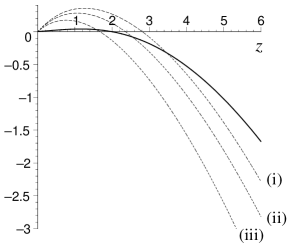
Fig. 7 demonstrates that a very clear signal of differences in the redshift time drift between the timescape model and CDM models might be determined at low redshifts when should be positive. In particular, the magnitude of is considerably smaller for the timescape model as compared to CDM models. Observationally, however, it is expected that measurements will be best determined for sources in the Lyman forest in the range, . At such redshifts the magnitude of the drift is somewhat more pronounced in the case of the CDM models. For a source at , over a period of years we would have for the timescape model with and . By comparison, for a spatially flat CDM model with a source at would over ten years give for , and for .
4 Discussion
The tests outlined here demonstrate several lines of investigation to distinguish the timescape model from models of homogeneous dark energy. The (in)homogeneity test of Bassett, Clarkson and Lu is definitive, since it tests the validity of the Friedmann equation directly.
In performing these tests, however, one must be very careful to ensure that data has not been reduced with built–in assumptions that use the Friedmann equation. For example, current estimates of the BAO scale such as that of Percival et al. Percival do not determine directly from redshift and angular diameter measures, but first perform a Fourier space transformation to a power spectrum, assuming a FLRW cosmology. Redoing such analyses for the timescape model may involve a recalibration of relevant transfer functions.
In the case of supernovae, one must also take care as compilations such as the Union union and Constitution Hicken datasets use the SALT method to calibrate light curves. In this approach empirical light curve parameters and cosmological parameters – assuming the Friedmann equation – are simultaneously fit by analytic marginalisation before the raw apparent magnitudes are recalibrated. As Hicken et al. discuss Hicken , a number of systematic discrepancies exist between data reduced by the SALT, SALT2, MLCS31 and MLCS17 techniques even within the CDM model. In the case of the timescape model, we find considerable differences between the different approaches SW . In principle, at present there appear to be enough supernovae to decide between the CDM and timescape models on Bayesian evidence, but one is led to different conclusions depending on how the data is reduced. It is therefore important that the systematic issues are unravelled.
The value of the dressed Hubble constant is also an observable quantity of considerable interest. A recent determination of by Riess et al. shoes poses a challenge for the timescape model. However, it is a feature of the timescape model that a 17–22% variance in the apparent Hubble flow will exist on local scales below the scale of statistical homogeneity, and this may potentially complicate calibration of the cosmic distance ladder. Further quantification of the variance in the apparent Hubble flow in relationship to local cosmic structures would provide an interesting possibility for tests of the timescape cosmology for which there are no counterparts in the standard cosmology.
References
- (1) D.L. Wiltshire, Phys. Rev. D 80, 123512 (2009).
- (2) D.L. Wiltshire, in Dark Matter in Astroparticle and Particle Physics: Proc. of the 6th International Heidelberg Conference, eds H.V. Klapdor–Kleingrothaus and G.F. Lewis, (World Scientific, Singapore, 2008) pp. 565-596 [arXiv:0712.3984].
- (3) F. Hoyle and M.S. Vogeley, Astrophys. J. 566, 641 (2002); Astrophys. J. 607, 751 (2004).
- (4) T. Buchert, Gen. Relativ. Grav. 32, 105 (2000); Gen. Relativ. Grav. 33, 1381 (2001).
- (5) T. Buchert, Gen. Relativ. Grav. 40, 467 (2008).
- (6) P.J.E. Peebles, in this volume; arXiv:0910.5142.
- (7) D.L. Wiltshire, New J. Phys. 9, 377 (2007).
- (8) D.L. Wiltshire, Phys. Rev. Lett. 99, 251101 (2007).
- (9) D.L. Wiltshire, Phys. Rev. D 78, 084032 (2008).
- (10) B.M. Leith, S.C.C. Ng and D.L. Wiltshire, Astrophys. J. 672, L91 (2008).
- (11) S. Jha, A.G. Riess and R.P. Kirshner, Astrophys. J. 659, 122 (2007).
- (12) N. Li and D.J. Schwarz, Phys. Rev. D78, 083531 (2008).
- (13) E. Komatsu et al., Astrophys. J. Suppl. 180, 330 (2009).
- (14) A.G. Riess et al., Astrophys. J. 659, 98 (2007).
- (15) B.E. Schaefer, Astrophys. J. 660, 16 (2007); N. Liang, W. K. Xiao, Y. Liu and S.N. Zhang, Astrophys. J. 685, 354 (2008). L. Amati, C. Guidorzi, F. Frontera, M. Della Valle, F. Finelli, R. Landi and E. Montanari, Mon. Not. R. Astr. Soc. 391, 577 (2008); R. Tsutsui, T. Nakamura, D. Yonetoku, T. Murakami, Y. Kodama and K. Takahashi, JCAP 08 (2009) 015.
- (16) B.E. Schaefer, in preparation.
- (17) G.B. Zhao and X. Zhang, arXiv:0908.1568.
- (18) P. Serra, A. Cooray, D.E. Holz, A. Melchiorri, S. Pandolfi and D. Sarkar, arXiv:0908.3186.
- (19) E. Gaztañaga, A. Cabre and L. Hui, Mon. Not. R. Astr. Soc. 399, 1663 (2009).
- (20) J.A. Gu, C.W. Chen and P. Chen, New J. Phys. 11, 073029 (2009).
- (21) V. Sahni, A. Shafieloo and A. A. Starobinsky, Phys. Rev. D 78, 103502 (2008).
- (22) C. Zunckel and C. Clarkson, Phys. Rev. Lett. 101, 181301 (2008).
- (23) A. Shafieloo, V. Sahni and A.A. Starobinsky, Phys. Rev. D 80, 101301 (2009).
- (24) C. Alcock and B. Paczyński, Nature 281, 358 (1979).
- (25) D.J. Eisenstein et al., Astrophys. J. 633 (2005) 560; S. Cole et al., Mon. Not. R. Astr. Soc. 362 (2005) 505.
- (26) W.J. Percival et al., Mon. Not. R. Astr. Soc. 381, 1053 (2007); W.J. Percival et al., arXiv:0907.1660.
- (27) E. Gaztañaga, A. Cabré, F. Castander, M. Crocce and P. Fosalba, Mon. Not. R. Astr. Soc. 399, 801 (2009).
- (28) C. Clarkson, B. Bassett and T.C. Lu, Phys. Rev. Lett. 101, 011301 (2008).
- (29) A. Sandage, Astrophys. J. 136, 319 (1962); G.C. McVittie, Astrophys. J. 136, 334 (1962); A. Loeb, Astrophys. J. 499, L111 (1998).
- (30) J.P. Uzan, C. Clarkson and G.F.R. Ellis, Phys. Rev. Lett. 100, 191303 (2008).
- (31) P.S. Corasaniti, D. Huterer and A. Melchiorri, Phys. Rev. D75, 062001 (2007); J. Liske et al., Mon. Not. R. Astr. Soc. 386, 1192 (2008).
- (32) M. Kowalski et al., Astrophys. J. 686, 749 (2008).
- (33) M. Hicken et al., Astrophys. J. 700, 1097 (2009).
- (34) P.R. Smale and D.L. Wiltshire, in preparation.
- (35) A.G. Riess et al., Astrophys. J. 699, 539 (2009).