Holographic description of quantum field theory

Abstract

We propose that general $D$-dimensional quantum field theories are dual to $(D+1)$-dimensional local quantum theories which in general include objects with spin two or higher. Using a general prescription, we construct a $(D+1)$-dimensional theory which is holographically dual to the $D$-dimensional $O(N)$ vector model. From the holographic theory, the phase transition and critical properties of the model in dimensions $D>2$ are described.

I Introduction

Quantum field theory is a universal language that describes long wavelength fluctuations in quantum systems made of many degrees of freedom. Although strongly coupled quantum field theories commonly arise in nature, it is notoriously difficult to find a systematic way of understanding strongly coupled quantum field theories.

The anti-de Sitter space/conformal field theory correspondenceMALDACENA ; GUBSER ; WITTEN opened the door to understand a class of strongly coupled quantum field theories. According to the duality, certain strongly coupled quantum field theories in $D$ dimensions can be mapped into weakly coupled gravitational theories in $(D+1)$ dimensions in large $N$ limits. Although the original correspondence has been conjectured based on the superstring theory, it is possible that the underlying principle is more general and a wider class of quantum field theories can be understood through holographic descriptionsKLEBANOV ; DAS ; Gopakumar:2004qb ; POLCHINSKI09 , which may have different UV completion than the string theory.

In this paper, we provide a prescription to construct holographic theories for general quantum field theories. As a demonstration of the method, we explicitly construct a dual theory for the $D$-dimensional $O(N)$ vector model, and reproduce the phase transition and critical behaviors of the model using the holographic description.

The paper is organized in the following way. In Sec. II, we will convey the main idea behind the holographic description by constructing a dual theory for a toy model. In Sec. III A, using the general idea presented in Sec. II, we will explicitly construct a holographic theory dual to the $D$-dimensional $O(N)$ vector model. In Sec. III B, we will consider a large $N$ limit where the theory becomes classical for $O(N)$ singlet fields in the bulk. In Sec. III C, the phase transition and critical properties of the $O(N)$ model will be discussed using the holographic theory.

II Toy-model : $0$-dimensional scalar theory

In this section, we will construct a holographic theory for one of the simplest models : $0$-dimensional scalar theory. In zero dimension, the partition function is given by an ordinary integration,

$$Z[{\cal J}] = \int d\Phi~{}e^{-S[\Phi]}.$$ (1)

We consider an action $S[\Phi]=S_{M}[\Phi]+S_{\cal J}[\Phi]$ with

$$S_{M}[\Phi] = M^{2}\Phi^{2},$$

$$S_{\cal J}[\Phi] = \sum_{n=1}^{\infty}{\cal J}_{n}\Phi^{n}.$$ (2)

Here $S_{M}$ is the bare action with ‘mass’ $M$. $S_{\cal J}$ is a deformation with sources ${\cal J}_{n}$. The values of ${\cal J}_{n}$’s are not necessarily small. In the following, we will consider deformations upto quartic order : ${\cal J}_{n}=0$ for $n>4$. However, the following discussion can be straightforwardly generalized to more general cases.

For a given set of sources ${\cal J}_{n}$, quantum fluctuations are controlled by the bare mass $M$. One useful way of organizing quantum fluctuations is to separate high energy modes and low energy modes, and include high energy fluctuations through an effective action for the low energy modes. Although there is only one scalar variable in this case, this can be done through the Polchinski’s renormalization group schemePOLCHINSKI84 . First, an auxiliary field $\tilde{\Phi}$ with mass $\mu$ is introduced,

$$Z[{\cal J}] = \mu\int d\Phi d\tilde{\Phi}~{}e^{-(S[\Phi]+\mu^{2}\tilde{\Phi}^{2})}.$$ (3)

At this stage, $\tilde{\Phi}$ is a pure auxiliary field without any physical significance. Then, we find a new basis $\phi$ and $\tilde{\phi}$

$$\Phi = \phi+\tilde{\phi},$$

$$\tilde{\Phi} = A\phi+B\tilde{\phi},$$ (4)

in such a way that the ‘low energy field’ $\phi$ has a mass $M^{{}^{\prime}}$ which is slightly larger than the original mass $M$. As a result, quantum fluctuations for $\phi$ become slightly smaller than the original field $\Phi$. The missing quantum fluctuations are compensated by the ‘high energy field’ $\tilde{\phi}$ with mass $m^{{}^{\prime}}$. If we choose the mass of the low energy field $\phi$ as

$$M^{{}^{\prime}2} = M^{2}e^{2\alpha dz}$$ (5)

with $dz$ being an infinitesimally small parameter and $\alpha$ being a positive constant, we have to choose

$$A=-\frac{MM^{{}^{\prime}}}{m^{{}^{\prime}}\mu},~{}~{}B=\frac{m^{{}^{\prime}}M}{M^{{}^{\prime}}\mu},$$ (6)

where

$$m^{{}^{\prime}2} = M^{2}\frac{e^{2\alpha dz}}{e^{2\alpha dz}-1}=\frac{M^{2}}{2\alpha dz}.$$ (7)

Note that $m^{{}^{\prime}2}$ is very large, proportional to $1/dz$. This is because $\tilde{\phi}$ carries away only infinitesimally small quantum fluctuations of the original field $\Phi$. Moreover, $m^{{}^{\prime}}$ is independent of the arbitrary mass $\mu$ because $\tilde{\phi}$ is physical.

In terms of the new variables, the partition function is written as

$$Z[{\cal J}] = \left(\frac{Mm^{{}^{\prime}}}{M^{{}^{\prime}}}+\frac{MM^{{}^{\prime}}}{m^{{}^{\prime}}}\right)\int d\phi d\tilde{\phi}~{}e^{-(S_{\cal J}[\phi+\tilde{\phi}]+M^{{}^{\prime}2}\phi^{2}+m^{{}^{\prime}2}\tilde{\phi}^{2})}.$$ (8)

If we rescale the fields,

$$\phi\rightarrow e^{-\alpha dz}\phi,~{}~{}~{}~{}\tilde{\phi}\rightarrow e^{-\alpha dz}\tilde{\phi},$$ (9)

the quadratic action for low energy field $\phi$ can be brought into the form which is the same as the original bare action,

$$Z[{\cal J}] = m\int d\phi d\tilde{\phi}~{}e^{-(S_{j}[\phi+\tilde{\phi}]+M^{2}\phi^{2}+m^{2}\tilde{\phi}^{2})},$$ (10)

where

$$S_{j}[\phi+\tilde{\phi}] = \sum_{n=1}^{4}j_{n}(\phi+\tilde{\phi})^{n},$$ (11)

with $j_{n}={\cal J}_{n}e^{-n\alpha dz}$ and $m=m^{{}^{\prime}}e^{-\alpha dz}$. Note that $j_{n}$’s become smaller than the original sources ${\cal J}_{n}$, which is a manifestation of reduced quantum fluctuations for the low energy field $\phi$. The new action can be expanded in power of the low energy field,

$$S_{j}[\phi+\tilde{\phi}] = S_{j}[\tilde{\phi}]+(j_{1}+2j_{2}\tilde{\phi}+3j_{3}\tilde{\phi}^{2}+4j_{4}\tilde{\phi}^{3})\phi$$ (12)

$$+(j_{2}+3j_{3}\tilde{\phi}+6j_{4}\tilde{\phi}^{2})\phi^{2}+(j_{3}+4j_{4}\tilde{\phi})\phi^{3}+j_{4}\phi^{4}.$$

In the standard renormalization group (RG) procedurePOLCHINSKI84 ; POLONYI , one integrates out the high energy field to obtain an effective action for the low energy field with renormalized coupling constants. Here we take an alternative view and interpret the high energy field $\tilde{\phi}$ as fluctuating sources for the low energy field. This means that the sources for the low energy field can be regarded as dynamical fields instead of fixed coupling constants. To make this more explicit, we decouple the high energy field and the low energy field by introducing Hubbard-Stratonovich fields $J_{n}$ and $P_{n}$,

$$Z[{\cal J}] = m\int d\phi d\tilde{\phi}\Pi_{n=1}^{4}(dJ_{n}dP_{n})~{}e^{-(S_{j}^{{}^{\prime}}+M^{2}\phi^{2}+m^{2}\tilde{\phi}^{2})},$$ (13)

where

$$S_{j}^{{}^{\prime}} = S_{j}[\tilde{\phi}]$$ (14)

$$+iP_{1}J_{1}-iP_{1}(j_{1}+2j_{2}\tilde{\phi}+3j_{3}\tilde{\phi}^{2}+4j_{4}\tilde{\phi}^{3})+J_{1}\phi$$

$$+iP_{2}J_{2}-iP_{2}(j_{2}+3j_{3}\tilde{\phi}+6j_{4}\tilde{\phi}^{2})+J_{2}\phi^{2}$$

$$+iP_{3}J_{3}-iP_{3}(j_{3}+4j_{4}\tilde{\phi})+J_{3}\phi^{3}$$

$$+iP_{4}J_{4}-iP_{4}j_{4}+J_{4}\phi^{4}.$$

Now we integrate out $\tilde{\phi}$ to obtain an effective action for the source fields. The mass $m^{2}$ for the high energy field is proportional to $1/dz$ and only terms that are linear in $dz$ contribute to the effective action (for the derivation, see the Appendix A),

$$Z[{\cal J}] = \int d\phi\Pi_{n=1}^{4}(dJ_{n}dP_{n})~{}e^{-(S_{J}[\phi]+M^{2}\phi^{2}+S^{(1)}[J,P])},$$ (15)

where

$$S^{(1)}[J,P] = \sum_{n=1}^{4}i(J_{n}-{\cal J}_{n}+n\alpha dz{\cal J}_{n})P_{n}$$ (16)

$$+\frac{\alpha dz}{2M^{2}}(i\tilde{\cal J}_{1}+2P_{1}\tilde{\cal J}_{2}+3P_{2}\tilde{\cal J}_{3}+4P_{3}\tilde{\cal J}_{4})^{2}$$

with $\tilde{\cal J}_{n}=({\cal J}_{n}+J_{n})/2$.

After repeating the steps from Eqs. (3) to (15) $R$ times, one obtains a path integral for the partition function

$$Z[{\cal J}] = \int\Pi_{k=1}^{R}\Pi_{n=1}^{4}(DJ_{n}^{(k+1)}DP_{n}^{(k)})e^{-S^{(R)}[J^{(k)},P^{(k)}]}Z[J^{(R+1)}],$$ (17)

where

$$S^{(R)}[J^{(k)},P^{(k)}] = \sum_{k=1}^{R}\Bigl{[}\sum_{n=1}^{4}i(J_{n}^{(k+1)}-J_{n}^{(k)}+n\alpha dzJ_{n}^{(k)})P_{n}^{(k)}$$ (18)

$$+\frac{\alpha dz}{2M^{2}}(i\tilde{J}_{1}^{(k)}+2P_{1}^{(k)}\tilde{J}_{2}^{(k)}+3P_{2}^{(k)}\tilde{J}_{3}^{(k)}+4P_{3}^{(k)}\tilde{J}_{4}^{(k)})^{2}\Bigr{]}$$

with $\tilde{J}_{n}^{(k)}=(J_{n}^{(k+1)}+J_{n}^{(k)})/2$ and $J_{n}^{(1)}={\cal J}_{n}$. The non-trivial solution for Eq. (17) is given by

$$Z[{\cal J}] = \int\Pi_{n=1}^{4}(DJ_{n}DP_{n})~{}e^{-S[J,P]},$$ (19)

where

$$S[J,P] = \int_{0}^{\infty}dz\Bigl{[}i(\partial_{z}J_{n}+n\alpha J_{n})P_{n}$$ (20)

$$+\frac{\alpha}{2M^{2}}(iJ_{1}+2P_{1}J_{2}+3P_{2}J_{3}+4P_{3}J_{4})^{2}\Bigr{]}.$$

Here $DJ_{n}DP_{n}$ represent functional integrations over one dimensional fields $J_{n}(z),P_{n}(z)$ which are defined on the semi-infinite line $[0,\infty)$. The boundary value of $J_{n}(z)$ is fixed by the coupling constants of the original theory, $J_{n}(0)={\cal J}_{n}$. $P_{n}(z)$ is the conjugate field of $J_{n}(z)$. The physical meaning of $P_{n}$ becomes clear from the equation of motion for the corresponding source field. By taking derivative of Eq. (14) with respect to $J_{n}$, one obtains

$$<\phi^{n}>=-i<P_{n}>.$$ (21)

Therefore, $P_{n}$ describes physical fluctuations of the operator $\phi^{n}$, and an expectation value of $P_{n}$ along the imaginary axis gives an expectation value of the operator.

The theory given by Eqs. (19) and (20), which is exactly dual to the original theory, is an one-dimensional local quantum theory. The emergent dimension $z$ corresponds to logarithmic energy scaleVERLINDE . The parameter $\alpha$ determines the rate the energy scale is changed. Despite the apparent similarity with the standard RG theory, there is an important difference. In the usual RG approach, quantum fluctuations of high energy modes modify coupling constants for low energy modes and generated new terms in the effective action. In the present approach, new terms are not generated and the structure of the bare theory is maintained at each level. In particular, the highest order coupling ($J_{4}$ in this case) obeys the strict constraint,

$$\partial_{z}J_{4}+4\alpha J_{4}=0$$ (22)

which is nothing but the classical scaling. This is because there is no dynamics for the conjugate field $P_{4}$ for the highest order coupling. Instead, other couplings acquire non-trivial dynamics and some of them become propagating modes in the bulk. Fluctuations of those dynamical coupling fields embody quantum fluctuations in this approach.

In quantum field theory, there is a redundancy as to what energy scale one should use to define theory. This makes the reparametrization of the RG flow to be a gauge symmetry. Because of this redundancy, the partition function in Eq. (19) does not depend on the rate high energy modes are eliminated as far as all modes are eventually eliminated. Moreover, at each step of mode elimination, one could have chosen $\alpha$ differently. Therefore, $\alpha$ can be regarded as a function of $z$. If one interprets $z$ as ‘time’, it is natural to identify $\alpha(z)$ as the ‘lapse function’, that is, $\alpha(z)=\sqrt{g_{zz}(z)}$, where $g_{zz}(z)$ is the metric. Then one can view Eqs. (19) and (20) as an one-dimensional gravitational theory with matter fields $J_{n}$. This becomes more clear if we write the Lagrangian as

$$L=P_{n}\partial_{z}J_{n}-\alpha H,$$ (23)

where $H$ is the Hamiltonian (the reason why $H$ is not Hermitian in this case is that we started from the Euclidean field theory). However, there is one important difference from the usual gravitational theory. In the Hamiltonian formalism of gravityADM , the lapse function is a Lagrangian multiplier which imposes the constraint $H=0$. However, in Eq. (19), $\alpha$ is not integrated over and the Hamiltonian constraint is not imposed. This is due to the presence of the boundary at $z=0$ which explicitly breaks the reparametrization symmetry. In particular, the ‘proper time’ from $z=0$ to $z=\infty$ given by

$$l=\int_{0}^{\infty}\alpha(z)dz$$ (24)

is a quantity of physical significance which measures the total warping factor. To reproduce the original partition function in Eq. (1) from Eq. (19), one has to make sure that $l=\infty$ to include all modes in the infrared limit. Therefore, $l$ should be fixed to be infinite. As a result, one should not integrate over all possible $\alpha(z)$ some of which give different $l$. This is the physical reason why the Hamiltonian constraint is not imposed in the present theory. This theory is a gravitational theory with the fixed size along the $z$ direction. Nonetheless, the partition function does not depend on a specific choice of $\alpha(z)$ as far as $l$ is fixed. If one wants to make this gauge symmetry more explicit, one could integrate in the gauge degree of freedom by summing over different $\alpha(z)$ with fixed $l$. For example, we can integrate over $\kappa_{z_{1},z_{2}}$ parametrizing $l$-preserving fluctuations of $\alpha$ as

$$\alpha(z)=\alpha_{0}(z)+\kappa_{z_{1},z_{2}}(\delta(z-z_{1})-\delta(z-z_{2})),$$ (25)

where $\alpha_{0}(z)$ is a ‘gauge fixed’ lapse function. Integration over $\kappa_{z_{1},z_{2}}$ generates the constraint

$$H(z_{1})=H(z_{2}).$$ (26)

However, this is a trivial constraint which is already implemented in Eq. (19) with fixed $\alpha$, because it is simply the conservation of ‘energy’.

Although there are many fields in the bulk, i.e. $J_{n},P_{n}$ for each $n$, there is only one propagating mode, and the remaining fields are non-dynamical in the sense they strictly obey constraints imposed by their conjugate fields. This is not surprising because we started with one dynamical field $\Phi$. There is a freedom in choosing one independent field. In this case, it is convenient to choose $J_{3}$ as an independent field because the conjugate field $P_{3}$ is multiplied by $J_{4}$ in Eq. (20), where $J_{4}$ is non-dynamical due to Eq. (22). Integrating over $P_{3}$, one obtains

$$S = \int_{0}^{\infty}dz\Bigl{[}\frac{M^{2}}{32\alpha J_{4}^{2}}(\partial_{z}J_{3}+3\alpha J_{3})^{2}-\frac{i}{4J_{4}}(\partial_{z}J_{3}+3\alpha J_{3})(3J_{3}P_{2}+2J_{2}P_{1}+iJ_{1})$$ (27)

$$~{}~{}~{}~{}~{}~{}~{}~{}~{}~{}~{}+i(\partial_{z}J_{1}+\alpha J_{1})P_{1}+i(\partial_{z}J_{2}+2\alpha J_{2})P_{2}\Bigr{]}.$$

$P_{1}$ and $P_{2}$ are Lagrangian multipliers which impose the constraints,

$$(\partial_{z}J_{1}+\alpha J_{1}) = \frac{J_{2}}{2J_{4}}(\partial_{z}J_{3}+3\alpha J_{3}),$$

$$(\partial_{z}J_{2}+2\alpha J_{2}) = \frac{3J_{3}}{4J_{4}}(\partial_{z}J_{3}+3\alpha J_{3}).$$ (28)

Remarkably, these constraints have a local solution, that is, the fields $J_{1}$ and $J_{2}$ at a scale $z$ depend only on the independent field $J_{3}$ at the same scale,

$$J_{1} = \frac{J_{3}^{3}}{16J_{4}^{2}}+{\cal J}_{2}e^{-2\alpha z}\frac{J_{3}}{2J_{4}},$$

$$J_{2} = \frac{3J_{3}^{2}}{8J_{4}}+{\cal J}_{2}e^{-2\alpha z}.$$ (29)

This locality is guaranteed because all source fields at a given scale are tied with one fluctuating field $\tilde{\phi}$ at the same scale. Here we considered the case with $Z_{2}$ symmetry where ${\cal J}_{n}=0$ for odd $n$. From this one can write down the local action for the independent field $J_{3}$ in the bulk,

$$S = \int_{0}^{\infty}dz\left[\frac{M^{2}}{32\alpha J_{4}^{2}}(\partial_{z}J_{3}+3\alpha J_{3})^{2}+\partial_{z}\left\{\frac{J_{3}^{4}}{256J_{4}^{3}}+\frac{{\cal J}_{2}e^{-2\alpha z}}{16J_{4}^{2}}J_{3}^{2}\right\}\right].$$ (30)

The first term is a bulk term and the second term is a boundary term. Since $J_{3}(z=0)=0$, the boundary terms contribute only at the infrared limit $z=\infty$. The theory for $J_{3}$ is free in the bulk, but the boundary term contains non-trivial interactions. Presumably, this theory is not easier to solve than the original theory due to the boundary interactions. However, the construction of the dual theory for the toy model illustrates how one can construct dual theories for more general field theories. Now, rather than trying to analyze the theory (30), we will move on to apply the prescription to more non-trivial field theory : $D$-dimensional $O(N)$ vector model.

III $D$-dimensional O(N) vector theory

III.1 Construction of dual theory

We consider a $D$-dimensional vector field theory,

$$Z[{\cal J}] = \int D\Phi_{a}~{}e^{-(S_{M}[\Phi]+S_{\cal J}[\Phi])},$$ (31)

where

$$S_{M}[\Phi] = \int d{\bf x}d{\bf y}~{}\Phi_{a}({\bf x})G_{M}^{-1}({\bf x}-{\bf y})\Phi_{a}({\bf y}),$$

$$S_{\cal J}[\Phi] = \int d{\bf x}~{}\Bigl{[}{\cal J}_{a}\Phi_{a}+{\cal J}_{ab}\Phi_{a}\Phi_{b}+{\cal J}_{abc}\Phi_{a}\Phi_{b}\Phi_{c}+{\cal J}_{abcd}\Phi_{a}\Phi_{b}\Phi_{c}\Phi_{d}$$ (32)

$$+{\cal J}_{ab}^{ij}\partial_{i}\Phi_{a}\partial_{j}\Phi_{b}+{\cal J}_{abc}^{ij}\Phi_{a}\partial_{i}\Phi_{b}\partial_{j}\Phi_{c}+{\cal J}_{abcd}^{ij}\Phi_{a}\Phi_{b}\partial_{i}\Phi_{c}\partial_{j}\Phi_{d}\Bigr{]}.$$

Here $\int d{\bf x}$ and $\int d{\bf y}$ are integrations on a $D$-dimensional manifold ${\cal M}^{D}$. Here we use ${\cal M}^{D}=\mathbb{R}^{D}$ for simplicity. $\Phi_{a}$ is $O(N)$ vector field. $G_{M}^{-1}({\bf x})$ is the regularized kinetic energy with

$$G_{M}^{-1}({\bf x}) = \int d{\bf p}~{}p^{2}K^{-1}\left(p/M\right)e^{ipx},$$ (33)

where $px\equiv p_{i}x_{i}$. $K^{-1}(s)$ is an analytic function of $s^{2}$, which remains to be order of $1$ for $s<1$ and grows smoothly for $s>1$, for example,

$$K^{-1}(s) = e^{s^{2}}.$$ (34)

The mass scale $M$ is a UV cut-off above which fluctuations of $\Phi_{a}$ are suppressed. $S_{\cal J}$ is a deformation of the free theory. We consider sources ${\cal J}_{ab...}$ which are fully symmetric in the flavor indices $a,b,...$. In general, the sources may depend on ${\bf x}$. Although we can add more general deformations, we will proceed with this quartic action (32) which is sufficient to illustrate general features of the holographic description.

To integrate out high energy modes, we add an auxiliary vector field $\tilde{\Phi}_{a}$,

$$Z[{\cal J}] = [\det\tilde{G}_{D}]^{-N/2}\int D\Phi D\tilde{\Phi}~{}e^{-(S_{M}[\Phi]+S_{\cal J}[\Phi]+\tilde{S}[\tilde{\Phi}])},$$ (35)

where

$$\tilde{S}[\tilde{\Phi}] = \int d{\bf x}d{\bf y}~{}\tilde{\Phi}_{a}({\bf x})\tilde{G}^{-1}_{D}({\bf x}-{\bf y})\tilde{\Phi}_{a}({\bf y}).$$ (36)

The form of the propagator $\tilde{G}_{D}$ for the auxiliary field does not affect the final answer. Then, we find a new basis $\phi$ and $\tilde{\phi}$,

$$\Phi_{a}({\bf x}) = \phi_{a}({\bf x})+\tilde{\phi}_{a}({\bf x}),$$

$$\tilde{\Phi}_{a}({\bf x}) = \int d{\bf y}~{}\left(A({\bf x},{\bf y})\phi_{a}({\bf y})+B({\bf x},{\bf y})\tilde{\phi}_{a}({\bf y})\right),$$ (37)

where $A$ and $B$ are chosen to satisfy

$$G_{M}^{-1}+A^{T}\tilde{G}_{D}^{-1}A = G^{-1}_{M^{{}^{\prime}}},$$

$$G_{M}^{-1}+B^{T}\tilde{G}_{D}^{-1}B = \tilde{G}^{{}^{\prime}-1},$$

$$G_{M}^{-1}+A^{T}\tilde{G}_{D}^{-1}B = 0$$ (38)

so that the low energy field $\phi$ has a slightly smaller UV cut-off $M^{{}^{\prime}}=Me^{-\alpha dz}$ and the high energy field $\tilde{\phi}$ has a propagator $\tilde{G}^{{}^{\prime}}=-(G_{M^{{}^{\prime}}}-G_{M})$. Then the partition function can be written as

$$Z[{\cal J}] = [\det\tilde{G}^{{}^{\prime}-1}\det G^{-1}_{M^{{}^{\prime}}}\det G_{M}]^{N/2}\int D\phi D\tilde{\phi}~{}e^{-(S_{\cal J}[\phi+\tilde{\phi}]+S_{M^{{}^{\prime}}}[\phi]+\tilde{S}^{{}^{\prime}}[\tilde{\phi}])},$$ (39)

where

$$\tilde{S}^{{}^{\prime}} = \int d{\bf x}d{\bf y}~{}\tilde{\phi}_{a}({\bf x})\tilde{G}^{{}^{\prime}-1}({\bf x}-{\bf y})\tilde{\phi}_{a}({\bf y}).$$ (40)

A rescaling of ${\bf x}$ and the fields,

$${\bf x} \rightarrow e^{\alpha dz}{\bf x},$$

$$\phi_{a} \rightarrow e^{(2-d)\alpha dz/2}\phi_{a},$$

$$\tilde{\phi}_{a} \rightarrow e^{(2-d)\alpha dz/2}\tilde{\phi}_{a}$$ (41)

brings the kinetic energy for the low energy field to the original form as

$$Z[{\cal J}] = [\det\tilde{G}^{-1}]^{N/2}\int D\phi D\tilde{\phi}~{}e^{-(S_{j}[\phi+\tilde{\phi}]+S_{M}[\phi]+\tilde{S}[\tilde{\phi}])},$$ (42)

where

$$S_{j}[\phi] = \int d{\bf x}~{}\Bigl{[}j_{a}\phi_{a}+j_{ab}\phi_{a}\phi_{b}+j_{abc}\phi_{a}\phi_{b}\phi_{c}+j_{abcd}\phi_{a}\phi_{b}\phi_{c}\phi_{d}$$ (43)

$$+j_{ab}^{ij}\partial_{i}\phi_{a}\partial_{j}\phi_{b}+j_{abc}^{ij}\phi_{a}\partial_{i}\phi_{b}\partial_{j}\phi_{c}+j_{abcd}^{ij}\phi_{a}\phi_{b}\partial_{i}\phi_{c}\partial_{j}\phi_{d}\Bigr{]}$$

with

$$j_{a}({\bf x}) = e^{\frac{2+D}{2}\alpha dz}~{}{\cal J}_{a}(e^{\alpha dz}{\bf x}),$$

$$j_{ab}({\bf x}) = e^{2\alpha dz}~{}{\cal J}_{ab}(e^{\alpha dz}{\bf x}),$$

$$j_{abc}({\bf x}) = e^{\frac{6-D}{2}\alpha dz}~{}{\cal J}_{abc}(e^{\alpha dz}{\bf x}),$$

$$j_{abcd}({\bf x}) = e^{(4-D)\alpha dz}~{}{\cal J}_{abcd}(e^{\alpha dz}{\bf x}),$$

$$j^{ij}_{ab}({\bf x}) = {\cal J}^{ij}_{ab}(e^{\alpha dz}{\bf x}),$$

$$j^{ij}_{abc}({\bf x}) = e^{\frac{2-d}{2}\alpha dz}~{}{\cal J}^{ij}_{abc}(e^{\alpha dz}{\bf x}),$$

$$j^{ij}_{abcd}({\bf x}) = e^{(2-d)\alpha dz}~{}{\cal J}^{ij}_{abcd}(e^{\alpha dz}{\bf x})$$ (44)

and

$$\tilde{G}^{-1}({\bf x}-{\bf y})=e^{(2+d)\alpha dz}\tilde{G}^{{}^{\prime}-1}(e^{\alpha dz}({\bf x}-{\bf y})).$$ (45)

The new action can be expanded in power of the low energy field,

$$S_{j}[\phi+\tilde{\phi}] = S_{j}[\tilde{\phi}]$$ (46)

$$+\int d{\bf x}\Bigl{\{}\Bigl{[}j_{a}+2j_{ab}\tilde{\phi}_{b}+3j_{abc}\tilde{\phi}_{b}\tilde{\phi}_{c}+4j_{abcd}\tilde{\phi}_{b}\tilde{\phi}_{c}\tilde{\phi}_{d}$$

$$~{}~{}-2\partial_{i}(j_{ab}^{ij}\partial_{j}\tilde{\phi}_{b})+j_{abc}^{ij}\partial_{i}\tilde{\phi}_{b}\partial_{j}\tilde{\phi}_{c}-2\partial_{i}(j_{abc}^{ij}\tilde{\phi}_{b}\partial_{j}\tilde{\phi}_{c})$$

$$~{}~{}+2j_{abcd}^{ij}\tilde{\phi}_{b}\partial_{i}\tilde{\phi}_{c}\partial_{j}\tilde{\phi}_{d}-2\partial_{i}(j_{abcd}^{ij}\tilde{\phi}_{b}\tilde{\phi}_{c}\partial_{j}\tilde{\phi}_{d})\Bigr{]}\phi_{a}$$

$$+\Bigl{[}j_{ab}+3j_{abc}\tilde{\phi}_{c}+6j_{abcd}\tilde{\phi}_{c}\tilde{\phi}_{d}-\partial_{i}(j_{abc}^{ij}\partial_{j}\tilde{\phi}_{c})$$

$$~{}~{}+j_{abcd}^{ij}\partial_{i}\tilde{\phi}_{c}\partial_{j}\tilde{\phi}_{d}-2\partial_{i}(j_{abcd}^{ij}\tilde{\phi}_{c}\partial_{j}\tilde{\phi}_{d})\Bigr{]}\phi_{a}\phi_{b}$$

$$+\Bigl{[}j_{ab}^{ij}+j_{abc}^{ij}\tilde{\phi}_{c}+j_{abcd}^{ij}\tilde{\phi}_{c}\tilde{\phi}_{d}\Bigr{]}\partial_{i}\phi_{a}\partial_{j}\phi_{b}$$

$$+\Bigl{[}j_{abc}+4j_{abcd}\tilde{\phi}_{d}-\frac{2}{3}\partial_{i}(j_{abcd}^{ij}\partial_{j}\tilde{\phi}_{d})\Bigr{]}\phi_{a}\phi_{b}\phi_{c}$$

$$+\Bigl{[}j_{abc}^{ij}+2j_{abcd}^{ij}\tilde{\phi}_{d}\Bigr{]}\phi_{a}\partial_{i}\phi_{b}\partial_{j}\phi_{c}$$

$$+j_{abcd}\phi_{a}\phi_{b}\phi_{c}\phi_{d}+j_{abcd}^{ij}\phi_{a}\phi_{b}\partial_{i}\phi_{c}\partial_{j}\phi_{d}\Bigr{\}}.$$

Here we ignored boundary terms in the $D$-dimensional space, assuming that the boundary is at infinity where couplings vanish. We decouple the low energy field and the high energy field by introducing Hubbard-Stratonovich fields,

$$Z[{\cal J}] = [\det\tilde{G}^{-1}]^{N/2}\int D\phi D\tilde{\phi}DJDP~{}e^{-(S_{j}^{{}^{\prime}}+S_{M}[\phi]+\tilde{S}[\tilde{\phi}])},$$ (47)

where

$$S_{j}^{{}^{\prime}} = S_{j}[\tilde{\phi}]$$ (48)

$$=\int d{\bf x} \Bigl{\{}iP_{a}J_{a}-iP_{a}\Bigl{[}j_{a}+2j_{ab}\tilde{\phi}_{b}+3j_{abc}\tilde{\phi}_{b}\tilde{\phi}_{c}+4j_{abcd}\tilde{\phi}_{b}\tilde{\phi}_{c}\tilde{\phi}_{d}$$

$$~{}~{}-2\partial_{i}(j_{ab}^{ij}\partial_{j}\tilde{\phi}_{b})+j_{abc}^{ij}\partial_{i}\tilde{\phi}_{b}\partial_{j}\tilde{\phi}_{c}-2\partial_{i}(j_{abc}^{ij}\tilde{\phi}_{b}\partial_{j}\tilde{\phi}_{c})$$

$$~{}~{}+2j_{abcd}^{ij}\tilde{\phi}_{b}\partial_{i}\tilde{\phi}_{c}\partial_{j}\tilde{\phi}_{d}-2\partial_{i}(j_{abcd}^{ij}\tilde{\phi}_{b}\tilde{\phi}_{c}\partial_{j}\tilde{\phi}_{d})\Bigr{]}+J_{a}\phi_{a}$$

$$+iP_{ab}J_{ab}-iP_{ab}\Bigl{[}j_{ab}+3j_{abc}\tilde{\phi}_{c}+6j_{abcd}\tilde{\phi}_{c}\tilde{\phi}_{d}-\partial_{i}(j_{abc}^{ij}\partial_{j}\tilde{\phi}_{c})$$

$$~{}~{}+j_{abcd}^{ij}\partial_{i}\tilde{\phi}_{c}\partial_{j}\tilde{\phi}_{d}-2\partial_{i}(j_{abcd}^{ij}\tilde{\phi}_{c}\partial_{j}\tilde{\phi}_{d})\Bigr{]}+J_{ab}\phi_{a}\phi_{b}$$

$$+iP_{ab,ij}J_{ab}^{ij}-iP_{ab,ij}\Bigl{[}j_{ab}^{ij}+j_{abc}^{ij}\tilde{\phi}_{c}+j_{abcd}^{ij}\tilde{\phi}_{c}\tilde{\phi}_{d}\Bigr{]}+J_{ab}^{ij}\partial_{i}\phi_{a}\partial_{j}\phi_{b}$$

$$+iP_{abc}J_{abc}-iP_{abc}\Bigl{[}j_{abc}+4j_{abcd}\tilde{\phi}_{d}-\frac{2}{3}\partial_{i}(j_{abcd}^{ij}\partial_{j}\tilde{\phi}_{d})\Bigr{]}+J_{abc}\phi_{a}\phi_{b}\phi_{c}$$

$$+iP_{abc,ij}J_{abc}^{ij}-iP_{abc,ij}\Bigl{[}j_{abc}^{ij}+2j_{abcd}^{ij}\tilde{\phi}_{d}\Bigr{]}+J_{abc}^{ij}\phi_{a}\partial_{i}\phi_{b}\partial_{j}\phi_{c}$$

$$+iP_{abcd}J_{abcd}-iP_{abcd}j_{abcd}+J_{abcd}\phi_{a}\phi_{b}\phi_{c}\phi_{d}$$

$$+iP_{abcd,ij}J_{abcd}^{ij}-iP_{abcd,ij}j_{abcd}^{ij}+J_{abcd}^{ij}\phi_{a}\phi_{b}\partial_{i}\phi_{c}\partial_{j}\phi_{d}.$$

Now we integrate out $\tilde{\phi}$, following the similar procedure as explained in the Appendix A to obtain

$$Z[{\cal J}] = \int d\phi DJDP~{}e^{-(S_{J}[\phi]+S_{M}[\phi]+S^{(1)}[J,P])},$$ (49)

where

$$S^{(1)}[J,P] =\int d{\bf x} \Bigl{\{}iP_{a}(\partial J_{a}-\frac{2+D}{2}\alpha{\cal J}_{a})+iP_{ab}(\partial J_{ab}-2\alpha{\cal J}_{ab})+iP_{ab,ij}(\partial J_{ab}^{ij})$$ (50)

$$+iP_{abc}(\partial J_{abc}-\frac{6-D}{2}\alpha{\cal J}_{abc})+iP_{abc,ij}(\partial J_{abc}^{ij}-\frac{2-d}{2}\alpha{\cal J}_{abc}^{ij})$$

$$+iP_{abcd}(\partial J_{abcd}-(4-D)\alpha{\cal J}_{abcd})+iP_{abcd,ij}(\partial J_{abcd}^{ij}-(2-d)\alpha{\cal J}_{abcd}^{ij})\Bigr{\}}dz$$

$$+\frac{1}{4}\int d{\bf x}d{\bf y} \Bigl{\{}s_{a}({\bf x})\tilde{G}({\bf x}-{\bf y})s_{a}({\bf y})\Bigr{\}}.$$

Here, $\partial=\frac{\partial}{\partial z}-\alpha\sum_{i=1}^{D}x_{i}\frac{\partial}{\partial x_{i}}$ and

$$s_{a} = \Bigl{[}i\tilde{\cal J}_{a}+2P_{b}\tilde{\cal J}_{ab}-2\partial_{j}(\tilde{\cal J}_{ab}^{ij}\partial_{i}P_{b})+3P_{bc}\tilde{\cal J}_{abc}-\partial_{j}(\tilde{\cal J}_{abc}^{ij}\partial_{i}P_{bc})$$ (51)

$$~{}~{}+P_{bc,ij}\tilde{\cal J}_{abc}^{ij}+4P_{bcd}\tilde{\cal J}_{abcd}-\frac{2}{3}\partial_{j}(\tilde{\cal J}_{abcd}^{ij}\partial_{i}P_{bcd})+2\tilde{\cal J}_{abcd}^{ij}P_{bcd,ij}\Bigr{]}$$

with $\tilde{\cal J}_{a..}=({\cal J}_{a..}+J_{a..})/2$ and $\tilde{\cal J}_{a..}^{ij}=({\cal J}_{a..}^{ij}+J_{a..}^{ij})/2$. If one integrate out $J$’s and $P$’s in Eq. (49), one reproduces the action obtained by integrating out $\tilde{\phi}$ in Eq. (42) to the order of $dz$. If we keep applying the same procedure to the action for the low energy field as we did in the previous section, the partition function can be written as

$$Z[{\cal J}] = \int DJDP~{}e^{-S[J,P]},$$ (52)

where the $(D+1)$-dimensional action is given by

$$S[J,P] =\int d{\bf x}dz \Bigl{\{}iP_{a}(\partial J_{a}-\frac{2+D}{2}\alpha J_{a})+iP_{ab}(\partial J_{ab}-2\alpha J_{ab})+iP_{ab,ij}(\partial J_{ab}^{ij})$$ (53)

$$+iP_{abc}(\partial J_{abc}-\frac{6-D}{2}\alpha J_{abc})+iP_{abc,ij}(\partial J_{abc}^{ij}-\frac{2-d}{2}\alpha J_{abc}^{ij})$$

$$+iP_{abcd}(\partial J_{abcd}-(4-D)\alpha J_{abcd})+iP_{abcd,ij}(\partial J_{abcd}^{ij}-(2-d)\alpha J_{abcd}^{ij})\Bigr{\}}$$

$$+\frac{1}{4}\int d{\bf x}d{\bf y}dz \Bigl{\{}\alpha s_{a}({\bf x})G^{{}^{\prime}}({\bf x}-{\bf y})s_{a}({\bf y})\Bigr{\}},$$

with

$$s_{a} = \Bigl{[}iJ_{a}+2P_{b}J_{ab}-2\partial_{j}(J_{ab}^{ij}\partial_{i}P_{b})+3P_{bc}J_{abc}-\partial_{j}(J_{abc}^{ij}\partial_{i}P_{bc})$$ (54)

$$~{}~{}+P_{bc,ij}J_{abc}^{ij}+4P_{bcd}J_{abcd}-\frac{2}{3}\partial_{j}(J_{abcd}^{ij}\partial_{i}P_{bcd})+2J_{abcd}^{ij}P_{bcd,ij}\Bigr{]},$$

and $G^{{}^{\prime}}({\bf x})\equiv M\partial_{M}G_{M}({\bf x})$. Here the partition function is given by the functional integrals of the source fields $J$ and their conjugate fields $P$ in the $(D+1)$-dimensional space ${\cal M}^{D}\times[0,\infty)$. If the $D$-dimensional manifold ${\cal M}^{D}$ has a finite volume $V$, the volume at scale $z$ is given by $Ve^{-\alpha Dz}$ because of the rescaling of space in Eq. (41). Since $G_{M}({\bf p})^{-1}$ is smooth in momentum space, the last term in Eq. (53) can be expressed in gradient expansion. Higher derivative terms are suppressed by $\left(\frac{\partial_{i}}{M}\right)^{n}$. Therefore the full theory is local in $(D+1)$-dimensional space. The locality along the emergent $z$ direction is due to the fact that physics at a given energy scale $E$ depends on higher energy physics only through physics at an infinitesimally higher energy scale $Ee^{\alpha dz}$.

As is the case in the $0$-dimensional theory discussed in the previous section, $\alpha$ can be regarded as the lapse function in a gravitational theory in $(D+1)$ dimensions, but the Hamiltonian constraint is not imposed because of the boundary at $z=0$. Moreover, there is no fluctuating shift function which imposes the momentum constraint $P_{i}=0$ in the usual gravitation theory. This is, again, due to fact that the boundary explicitly breaks the diffeomorphism symmetry and only the momentum conservation (not $P_{i}=0$) is implemented in the theory.

One key difference from the $0$-dimensional theory is that there exist bulk fields with non-trivial spins. In Eq. (53), there are spin two fields which are coupled to the energy momentum tensor at the boundary. In the presence of more general deformations in the boundary theory, one needs to introduce fields with higher spinsVASILIEV ; PETKOU .

III.2 Large $N$ limit

In this section, we will consider a large $N$ limit where the dual theory becomes classical for $O(N)$ singlet fields. To see this, one decomposes tensors with rank two or greater than two into traceless tensors with the same rank and tensors with lower ranks as

$$J_{ab} = J_{2}\delta_{ab}+\frac{1}{N}\bar{J}_{ab},$$

$$J_{abc} = \frac{1}{N}\left[J_{3a}\delta_{bc}+J_{3b}\delta_{ac}+J_{3c}\delta_{ab}\right]+\frac{1}{N^{2}}\bar{J}_{abc},$$

$$J_{abcd} = \frac{J_{4}}{N}(\delta_{ab}\delta_{cd}+\delta_{ac}\delta_{bd}+\delta_{ad}\delta_{bc}),$$

$$P_{ab} = P_{2}\delta_{ab}+\bar{P}_{ab},$$

$$P_{abc} = P_{3a}\delta_{bc}+P_{3b}\delta_{ac}+P_{3c}\delta_{ab}+\bar{P}_{abc},$$

$$P_{abcd} = P_{4}(\delta_{ab}\delta_{cd}+\delta_{ac}\delta_{bd}+\delta_{ad}\delta_{bc}),$$

$$J_{ab}^{ij} = J_{2}^{ij}\delta_{ab}+\frac{1}{N}\bar{J}_{ab}^{ij},$$

$$J_{abc}^{ij} = \frac{1}{N}\left[J_{3a}^{ij}\delta_{bc}+J_{3b}^{ij}\delta_{ac}+J_{3c}^{ij}\delta_{ab}\right]+\frac{1}{N^{2}}\bar{J}_{abc}^{ij},$$

$$J_{abcd}^{ij} = \frac{J_{4}^{ij}}{N}(\delta_{ab}\delta_{cd}+\delta_{ac}\delta_{bd}+\delta_{ad}\delta_{bc}),$$

$$P_{ab,ij} = P_{2,ij}\delta_{ab}+\bar{P}_{ab,ij},$$

$$P_{abc,ij} = P_{3a,ij}\delta_{bc}+P_{3b,ij}\delta_{ac}+P_{3c,ij}\delta_{ab}+\bar{P}_{abc,ij},$$

$$P_{abcd,ij} = P_{4,ij}(\delta_{ab}\delta_{cd}+\delta_{ac}\delta_{bd}+\delta_{ad}\delta_{bc}),$$ (55)

where the fields with the bar are traceless, $\bar{J}_{aa}=\bar{J}_{aab}=\bar{J}_{aa}^{ij}=\bar{J}_{aab}^{ij}=0$ and $\bar{P}_{aa}=\bar{P}_{aab}=\bar{P}_{aa,ij}=\bar{P}_{aab,ij}=0$. For the quartic couplings which are the highest order couplings, only the $O(N)$ invariant parts are kept, assuming that the bare quartic couplings are $O(N)$ invariant. Note that the structures of the highest order coupling fields are not modified at all $z$, which is not true for other coupling fields : for lower order couplings, non-singlet contributions are generated at low energy scales even though the bare couplings are $O(N)$ invariant. Now, we consider the large $N$ limit with fixed $J_{a}$, $J_{2}$, $\bar{J}_{ab}$, $J_{3a}$, $\bar{J}_{abc}$, $J_{4}$, $J_{2}^{ij}$, $\bar{J}_{ab}^{ij}$, $J_{3a}^{ij}$, $\bar{J}_{abc}^{ij}$, $J_{4}$, $J_{4}^{ij}$. In this limit, the leading order action becomes

$$S[J,P] =\int d{\bf x}dz \Bigl{\{}iP_{a}(\partial J_{a}-\frac{2+D}{2}\alpha J_{a})+iNP_{2}(\partial J_{2}-2\alpha J_{2})+i\frac{1}{N}\bar{P}_{ab}(\partial\bar{J}_{ab}-2\alpha\bar{J}_{ab})$$ (56)

$$+iNP_{2,ij}(\partial J_{2}^{ij})+i\frac{1}{N}\bar{P}_{ab,ij}(\partial\bar{J}_{ab}^{ij})$$

$$+i3P_{3a}(\partial J_{3a}-\frac{6-D}{2}\alpha J_{3a})+i\frac{1}{N^{2}}\bar{P}_{abc}(\partial\bar{J}_{abc}-\frac{6-D}{2}\alpha\bar{J}_{abc})$$

$$+i3P_{3a,ij}(\partial J_{3a}^{ij}-\frac{2-d}{2}\alpha J_{3a}^{ij})+i\frac{1}{N^{2}}\bar{P}_{abc,ij}(\partial\bar{J}_{abc}^{ij}-\frac{2-d}{2}\alpha\bar{J}_{abc}^{ij})$$

$$+i3NP_{4}(\partial J_{4}-(4-D)\alpha J_{4})+i3NP_{4,ij}(\partial J_{4}^{ij}-(2-d)\alpha J_{4}^{ij})\Bigr{\}}$$

$$+\frac{1}{4}\int d{\bf x}d{\bf y}dz \Bigl{\{}\alpha s_{a}({\bf x},z)G^{{}^{\prime}}({\bf x}-{\bf y})s_{a}({\bf y},z)\Bigr{\}},$$

where

$$s_{a} = \Bigl{[}iJ_{a}+2P_{a}J_{2}+\frac{2}{N}P_{b}\bar{J}_{ab}-2\partial_{j}(J_{2}^{ij}\partial_{i}P_{a})-\frac{2}{N}\partial_{j}(\bar{J}_{ab}^{ij}\partial_{i}P_{b})$$ (57)

$$+3P_{2}J_{3a}+\frac{6}{N}\bar{P}_{ab}J_{3b}+\frac{3}{N^{2}}\bar{P}_{bc}\bar{J}_{abc}$$

$$-\partial_{j}(J_{3a}^{ij}\partial_{i}P_{2})-\frac{2}{N}\partial_{j}(J_{3b}^{ij}\partial_{i}\bar{P}_{ba})-\frac{1}{N^{2}}\partial_{j}(\bar{J}_{abc}^{ij}\partial_{i}\bar{P}_{bc})$$

$$~{}~{}+P_{2,ij}J_{3a}^{ij}+\frac{2}{N}\bar{P}_{ab,ij}J_{3b}^{ij}+\frac{1}{N^{2}}\bar{P}_{bc,ij}\bar{J}_{abc}^{ij}$$

$$+12P_{3a}J_{4}-2\partial_{j}(J_{4}^{ij}\partial_{i}P_{3a})+6J_{4}^{ij}P_{3a,ij}\Bigr{]}.$$

In the large $N$ limit, the action is manifestly proportional to $N$. Therefore, one can ignore quantum fluctuations for singlet fields such as $J_{2}$ and $J_{2}^{ij}$, and it is enough to consider saddle point solutions for singlet fields to compute correlation functions of singlet operators. It would be natural to integrate out all non-singlet fields and obtain an effective theory for single fields alone. However, it turns out that the effective action for single fields become non-local in this $O(N)$ vector model. This is because there are light non-singlet fields in the bulk and integrating over those soft modes generates non-local correlations for singlet fields. This means that we should keep light non-singlet fields as ‘low energy degrees of freedom’ in the bulk description if we want to use a local description.

III.3 Phase Transition and Critical Behaviors

In this section, we will describe the phase transition and the critical properties of the model in $D>2$ using the holographic theory. To maintain the locality of the description, we will keep light non-singlet fields in the theory by choosing $J_{3a}$’s as independent fields. We will focus on the simple case where there is no deformation on the energy-momentum tensor, and all sources respect the O(N) symmetry,

$$J_{a}({\bf x},0) = 0,$$

$$J_{ab}({\bf x},0) = {\cal J}_{2}({\bf x})\delta_{ab},$$

$$J_{abc}({\bf x},0) = 0,$$

$$J_{abcd}({\bf x},0) = \frac{{\cal J}_{4}({\bf x})}{N}\left(\delta_{ab}\delta_{cd}+\delta_{ac}\delta_{bd}+\delta_{ad}\delta_{bc}\right)$$ (58)

with $J_{2}^{ij}=\bar{J}_{ab}^{ij}=J_{3a}^{ij}=\bar{J}_{abc}^{ij}=J_{4}^{ij}=0$. From now on, it will be assumed that ${\cal J}_{4}({\bf x})={\cal J}_{4}>0$ is $x$-independent, but ${\cal J}_{2}({\bf x})$, which may have either sign, is $x$-dependent in general. We first integrate over $P_{3a}$ to obtain

$$S[J,P] = \int d{\bf x}dz~{}~{}\Bigl{\{}iP_{a}(\partial J_{a}-\frac{2+D}{2}\alpha J_{a})+iNP_{2}(\partial J_{2}-2\alpha J_{2})+i\frac{1}{N}\bar{P}_{ab}(\partial\bar{J}_{ab}-2\alpha\bar{J}_{ab})$$ (59)

$$~{}~{}~{}~{}~{}~{}~{}~{}~{}~{}-i\frac{s_{a}^{{}^{\prime}}}{4J_{4}}(\partial J_{3a}-\frac{6-D}{2}\alpha J_{3a})+i\frac{1}{N^{2}}\bar{P}_{abc}(\partial\bar{J}_{abc}-\frac{6-D}{2}\alpha\bar{J}_{abc})$$

$$~{}~{}~{}~{}~{}~{}~{}~{}~{}~{}+i3NP_{4}(\partial J_{4}-(4-D)\alpha J_{4})\Bigr{\}}$$

$$+\frac{1}{16}\int d{\bf x}d{\bf y}dz~{}~{}C({\bf x},z)[\alpha G^{{}^{\prime}}({\bf x}-{\bf y})]^{-1}C({\bf y},z)\Bigr{\}},$$

where $C({\bf x},z)\equiv\frac{1}{J_{4}({\bf x},z)}\left(\partial J_{3a}({\bf x},z)-\frac{6-D}{2}\alpha J_{3a}({\bf x},z)\right)$ and

$$s_{a}^{{}^{\prime}} = \Bigl{[}iJ_{a}+2P_{a}J_{2}+\frac{2}{N}P_{b}\bar{J}_{ab}+3P_{2}J_{3a}+\frac{6}{N}\bar{P}_{ab}J_{3b}+\frac{3}{N^{2}}\bar{P}_{bc}\bar{J}_{abc}\Bigr{]}.$$ (60)

Now we integrate over $P_{a},P_{2},\bar{P}_{ab},\bar{P}_{abc},P_{4}$ to obtain constraints,

$$\left(\partial J_{a}-\frac{2+D}{2}\alpha J_{a}\right)-\frac{1}{4J_{4}}\left(\partial J_{3b}-\frac{6-D}{2}\alpha J_{3b}\right)\left(2J_{2}\delta_{ab}+\frac{2}{N}\bar{J}_{ab}\right) = 0,$$

$$N(\partial J_{2}-2\alpha J_{2})-\frac{3}{4J_{4}}\left(\partial J_{3a}-\frac{6-D}{2}\alpha J_{3a}\right)J_{3a} = 0,$$

$$\frac{1}{N}(\partial\bar{J}_{ab}-2\alpha\bar{J}_{ab})-\frac{3}{4NJ_{4}}\left(\partial J_{3a}-\frac{6-D}{2}\alpha J_{3a}\right)J_{3b}$$

$$-\frac{3}{4NJ_{4}}\left(\partial J_{3b}-\frac{6-D}{2}\alpha J_{3b}\right)J_{3a}-\frac{3}{4N^{2}J_{4}}\left(\partial J_{3c}-\frac{6-D}{2}\alpha J_{3c}\right)\bar{J}_{abc} = 0,$$

$$\partial\bar{J}_{abc}-\frac{6-D}{2}\alpha\bar{J}_{abc} = 0,$$

$$\partial J_{4}-(4-D)\alpha J_{4} = 0.$$ (61)

For the boundary condition (58), the solution for the constraints is given by

$$J_{a}({\bf x},z) = \frac{3}{16NJ_{4}({\bf x},z)^{2}}J_{3a}({\bf x},z)J_{3b}({\bf x},z)J_{3b}({\bf x},z)+\frac{J_{3a}({\bf x},z){\cal J}_{2}(e^{\alpha z}{\bf x})e^{2\alpha z}}{2J_{4}({\bf x},z)},$$

$$J_{2}({\bf x},z) = \frac{3}{8NJ_{4}({\bf x},z)}J_{3a}({\bf x},z)J_{3a}({\bf x},z)+{\cal J}_{2}(e^{\alpha z}{\bf x})e^{2\alpha z},$$

$$\bar{J}_{ab}({\bf x},z) = \frac{3}{4J_{4}({\bf x},z)}J_{3a}({\bf x},z)J_{3b}({\bf x},z),$$

$$\bar{J}_{abc}({\bf x},z) = 0,$$

$$J_{4}({\bf x},z) = {\cal J}_{4}e^{(4-D)\alpha z},$$ (62)

where all repeated indices are summed as usual. Using this result, one can eliminate all fields except for $J_{3a}$ to obtain the action,

$$S[J,P] = \int d{\bf x}dz~{}~{}\partial_{z}\left[\frac{{\cal J}_{2}(e^{\alpha z}{\bf x})e^{2\alpha z}}{16J_{4}^{2}}J_{3a}J_{3a}+\frac{3\left(J_{3a}J_{3a}\right)^{2}}{256NJ_{4}^{3}}\right]$$ (63)

$$+\frac{1}{16}\int d{\bf x}d{\bf y}dzC({\bf x},z)[\alpha G^{{}^{\prime}}({\bf x}-{\bf y})]^{-1}C({\bf y},z)\Bigr{\}}.$$

In the first line of the above expression, all fields which do not have an explicit argument are understood to be at $({\bf x},z)$. The first term is a boundary action and the second term is the bulk action. In the bulk, $J_{3a}$ is massless and its action is purely quadratic. Although the bulk theory is non-interacting, the boundary term has non-trivial interactions and quantum fluctuations for the non-singlet field are still important.

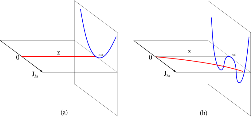
Figure 1: Saddle point configuration of $J_{3a}(z)$ (a) in the disordered phase and (b) in the ordered phase. Although the action is quadratic in $J_{3a}$ in the bulk, the boundary action drives the phase transition. When ${\cal J}_{2}$ is sufficiently negative, a Mexican-hat potential at the boundary drags $J_{3a}(z)$ away from $J_{3a}(z)=0$ in the bulk. At the critical point, $J_{3a}$ at the IR boundary $z=\infty$ is more or less free to fluctuate, generating algebraic correlations between fields inserted at the UV boundary $z=0$.

Due to the boundary term, the theory has a non-trivial phase transition. In the boundary term, the only contribution is from the infrared boundary, $z_{I}=\infty$ because there is no symmetry breaking source in the bare theory, $J_{3a}({\bf x},0)=0$. To discuss the phase transition, it is enough to consider $x$ independent singlet source fields ${\cal J}_{2}$ and ${\cal J}_{4}$. If ${\cal J}_{2}>{\cal J}_{2}^{c}$, where ${\cal J}_{2}^{c}\sim-{\cal J}_{4}M^{(D-2)}$ is a critical value, the boundary potential has the minimum at $J_{3a}=0$ as is shown in Fig. 1 (a). Therefore, the minimum energy configuration of $J_{3a}$ is the straight line along the $z$-direction. On the other hand, if ${\cal J}_{2}<{\cal J}_{2}^{c}$ the boundary term has the Mexican-hat potential. This causes the bulk field $J_{3a}$ to deviate from the trivial configuration $J_{3a}=0$, leading to the spontaneous symmetry breakingKLEBANOV99 as is shown in Fig. 1 (b). This describes the second order phase transition from the disordered phase to the ordered phase. We can use $-iP_{3a}\sim\phi^{2}\phi_{a}$ as an order parameter which roughly measures the slope of $J_{3a}(z)$ along the $z$ direction. In the phase with broken symmetry, $J_{3a}$ in the bulk is proportional to $\sqrt{N}$ and fluctuations away from the saddle point is $1/N$ suppressed, leading to the mean-field like critical exponent for the order parameter, $\beta=1/2$ in the large $N$ limit.

Now let us compute the two-point correlation function of the $O(N)$ singlet operator $\phi^{2}$ at the critical point. For this we integrate over $J_{3a}$ in the bulk in the presence of $x$-dependent source ${\cal J}_{2}({\bf x})={\cal J}^{c}_{2}+{\cal J}_{2}^{{}^{\prime}}({\bf x})$ with the boundary condition $J_{3a}({\bf x},0)=0$. Since the bulk action is quadratic one can use the saddle point solution in the bulk. In terms of the Fourier modes,

$$J_{3a}({\bf x},z)=\int d{\bf p}~{}~{}f_{a}({\bf p},z)e^{ipxe^{\alpha z}+(6-D)\alpha z/2},$$ (64)

the bulk action becomes

$$S_{bulk} = \frac{1}{16\alpha{\cal J}_{4}^{2}}\int dzd{\bf p}~{}~{}e^{-2\alpha z}[G^{{}^{\prime}}]^{-1}(pe^{\alpha z})[\partial_{z}f_{a}({\bf p},z)][\partial_{z}f_{a}(-{\bf p},z)].$$ (65)

The equation of motion for $f_{a}({\bf p},z)$ is

$$\partial_{z}\left(e^{-2\alpha z}G^{{}^{\prime}-1}(pe^{\alpha z})\partial_{z}f_{a}({\bf p},z)\right)=0.$$ (66)

There are two independent solutions : $1$ and $K(pe^{\alpha z}/M)$. The boundary condition at $z=0$ fixes only one coefficient, leading to one-parameter family of solutions given by

$$f_{a}({\bf p},z) = y_{a}({\bf p})\left[1-\frac{K\left(pe^{\alpha z}/M\right)}{K\left(p/M\right)}\right].$$ (67)

Here $K(s)$ is the regulator defined in Eq. (34), and $y_{a}({\bf p})$ is an arbitrary function. This arbitrariness is due to the fact that we have not imposed the boundary condition at the IR limit $z=\infty$. The condition of finiteness of the action alone does not fix the IR boundary condition because both independent solutions are regular in the IR limit. Here one should integrate over $y_{a}$ because $y_{a}$ is also a dynamical field. In this way, the boundary condition in the $IR$ limit is dynamically determined by the boundary action, whereas the boundary condition in the $UV$ is fixed by the bare coupling. Using the saddle point solution, one obtains an action for the boundary field $y_{a}$,

$$S = \frac{1}{16{\cal J}_{4}^{2}}\int d{\bf p}~{}~{}p^{2}K^{-1}(p/M)|y_{a}({\bf p})|^{2}$$ (68)

$$+\frac{1}{16{\cal J}_{4}^{2}}\int d{\bf p}_{1}d{\bf p}_{2}~{}~{}\left[{\cal J}_{2}^{c}\delta({\bf p}_{1}+{\bf p}_{2})+{\cal J}_{2}^{{}^{\prime}}(-{\bf p}_{1}-{\bf p}_{2})\right]y_{a}({\bf p}_{1})y_{a}({\bf p}_{2})$$

$$+\frac{3}{256N{\cal J}_{4}^{3}}\int d{\bf p}_{1}d{\bf p}_{2}d{\bf p}_{3}d{\bf p}_{4}~{}~{}\delta({\bf p}_{1}+{\bf p}_{2}+{\bf p}_{3}+{\bf p}_{4})y_{a}({\bf p}_{1})y_{a}({\bf p}_{2})y_{a}({\bf p}_{3})y_{a}({\bf p}_{4}).$$

Remarkably, this action has the same form as the original action for $\phi_{a}$, although this action is for the source field at the IR boundary. Despite the fact that it is no more convenient to use this dual description than using the conventional field theoretic method for the $O(N)$ model, one can proceed to integrate out the boundary field $y_{a}$, by summing over the usual chain diagrams, to obtain an effective potential $W[{\cal J}_{2}^{{}^{\prime}}({\bf q})]$ for the singlet field. From this, one can readily compute the correlation function. For example, in $D=3$ one obtains

$$\frac{\partial^{2}W}{\partial{\cal J}_{2}^{{}^{\prime}}({\bf q})\partial{\cal J}_{2}^{{}^{\prime}}(-{\bf q})}\sim|{\bf q}|+\mbox{(analytic terms)}$$ (69)

This leads to the scaling dimension $[\phi^{2}]=2$ as expected.

The fact that one has to solve essentially the same field theory to dynamically impose the IR boundary condition in the dual description is somewhat disappointing from the perspective of duality. However, this may have been expected in the $O(N)$ model. This is because all $N$ independent fields are massless, and we kept all of them in the local bulk effective action. Since no dynamical field has been integrated out, no information of the original theory has been coarse-grained and the bulk theory carries the exactly same amount of dynamical information as the original theory. An alternative approach would be to include more singlet fields such as $J_{2n}$ associated with the operators $(\phi_{a}^{2})^{n}$ for $n=1,2,...,N$, and integrate out all non-singlet fields to obtain an effective action for $N$ independent singlet fields. However, if one keeps only a small number of singlet fields and integrate out the remaining fields, the resulting action will not be local because their masses in the bulk are more or less equally spacedSEAN .

The holographic description for the $O(N)$ model is not very useful for practical purpose. After all, we can solve it in a much simpler way. We believe that the holographic approach may become more useful for more strongly interacting theories where there exist a gap between a small set of operators with small scaling dimensions and a large set of operators with large scaling dimensions. In such models, it is expected that quantum fluctuations of heavy propagating modes in the bulk will be encoded in local effective actions for light modes which carry dynamical information only for operators with small scaling dimensions. Then, imposing the IR boundary condition for the light modes may become more tractable than solving the original field theory.

IV Summary and Discussion

In the present paper, we provided a general prescription to construct holographic theory for general quantum field theory. Through an explicit construction, we showed that the holographic description for the $O(N)$ vector model correctly reproduce the spontaneous symmetry breaking phase transition and critical behaviors, as predicted by standard field theory methods. In the future, it is of great interest to apply this method to other strongly coupled quantum field theories where standard field theory techniques fail, such as matrix modelstHOOFT ; Gross:1990ub ; BERENSTEIN and non-Fermi liquids in 2+1 dimensions which are expected to be dual to certain matrix modelsSLEE09 .

If general quantum field theories in $D$ dimensions are holographically dual to certain $(D+1)$-dimensional local theories, the next question would be “What $(D+1)$-dimensional theories are dual to local $D$-dimensional quantum field theories ?” If one knows the answer to this question, one may use the holographic description to define quantum field theories and to classify them. To answer this question, it may be helpful to fully understand general structures behind the present holographic construction.

V Acknowledgment

The author thanks Allan Adams, Guido Festuccia, Sean Hartnoll, Igor Klebanov, Patrick Lee, Hong Liu, Joe Polchinski, T. Senthil, and Xiao-Gang Wen for illuminating discussions and comments. This research was supported by NSERC. The author also thanks KITP for its hospitality and the support through NSF Grant No. PHY05-51164 during the workshop, Quantum criticality and the AdS/CFT correspondence.

VI Appendix A

The action in Eq. (14) can be expanded in power of the high energy field as

$$S_{j}^{{}^{\prime}} = S_{J}[\phi]+\sum_{n=1}^{4}i(J_{n}-j_{n})P_{n}$$ (70)

$$+(j_{1}-2iP_{1}j_{2}-3iP_{2}j_{3}-4iP_{3}j_{4})\tilde{\phi}$$

$$+(j_{2}-3iP_{1}j_{3}-6iP_{2}j_{4})\tilde{\phi}^{2}$$

$$+(j_{3}-4iP_{1}j_{4})\tilde{\phi}^{3}$$

$$+j_{4}\tilde{\phi}^{4}.$$

Integrating over $\tilde{\phi}$ to the order of $1/m^{2}$, one obtains

$$Z[J] = \int d\phi\Pi_{n=1}^{4}(dJ_{n}dP_{n})~{}\frac{m}{\sqrt{m^{2}+B}}e^{-\left(M^{2}\phi^{2}+S_{J}[\phi]+i\sum_{n=1}^{4}(J_{n}-j_{n})P_{n}+\frac{A^{2}}{4(m^{2}+B)}\right)},$$ (71)

where

$$A = (ij_{1}+2P_{1}j_{2}+3P_{2}j_{3}+4P_{3}j_{4}),$$

$$B = (j_{2}-3iP_{1}j_{3}-6iP_{2}j_{4}).$$ (72)

The cubic and higher order terms in $\tilde{\phi}$ do not contribute to the linear order in $1/m^{2}\sim dz$. If we keep only those terms that are linear in $dz$ in Eq. (71), we obtain the action,

$$S=M^{2}\phi^{2}+S_{J}[\phi]+i\sum_{n=1}^{4}(J_{n}-j_{n})P_{n}+\frac{A^{2}}{4m^{2}}+\frac{B}{2m^{2}}.$$ (73)

However, it is not easy to take the continuum limit ($dz\rightarrow 0$) in this expression for the following reason. We can regard $j_{n}$ and $J_{n}$ as being defined at coordinates $z$ and $z+dz$ respectively, where $z$ is the logarithmic energy scale in the renormalization group flow. Then $P_{n}$ is defined in the interval (or at the middle point of the interval), $[z,z+dz]$. Usually, $A^{2}dz$ can be interpreted as the integration of $A^{2}$ between $z$ and $z+dz$ in the continuum limit. This would be the correct if $A$ were a fixed constant of the order of $1$. In the present case, however, $A$ contains the dynamical field $P_{n}$ whose typical amplitude is order of $m\sim\frac{1}{\sqrt{dz}}$. Therefore, an error of order of $1/m$ in $j_{n}$ in the integrand gives a non-trivial contribution to the integration, leading to a discrepancy between the result in Eq. (73) and the one obtained in the naive continuum limit.

To fix this problem, we consider the following trick. First we absorb the factor $\frac{1}{(m^{2}+B)}$ in front of $A^{2}$ in the action into the measure of $P_{3}$; we change the variable $P_{3}$ to $P_{3}^{{}^{\prime}}$ in Eq. (71),

$$P_{3} = \frac{\sqrt{m^{2}+B}}{m}P_{3}^{{}^{\prime}}+\frac{\sqrt{m^{2}+B}-m}{4mj_{4}}(ij_{1}+2P_{1}j_{2}+3P_{2}j_{3}),$$ (74)

which leads to

$$Z[J] = \int d\phi\Pi_{n\neq 3}(dJ_{n}dP_{n})dJ_{3}dP_{3}^{{}^{\prime}}~{}e^{-\left(M^{2}\phi^{2}+S_{J}[\phi]+S^{{}^{\prime}}\right)},$$ (75)

where

$$S^{{}^{\prime}} = i\sum_{n\neq 3}(J_{n}-j_{n})P_{n}+\frac{A^{{}^{\prime}2}}{4m^{2}}$$ (76)

$$+i(J_{3}-j_{3})\left(\frac{\sqrt{m^{2}+B}}{m}P_{3}^{{}^{\prime}}+\frac{\sqrt{m^{2}+B}-m}{4mj_{4}}(ij_{1}+2P_{1}j_{2}+3P_{2}j_{3})\right)$$

with $A^{{}^{\prime}}=(ij_{1}+2P_{1}j_{2}+3P_{2}j_{3}+4P_{3}^{{}^{\prime}}j_{4})$. If we take the leading order terms, the above expression becomes

$$S^{{}^{\prime}} = i\sum_{n\neq 3}(J_{n}-j_{n})P_{n}+\frac{A^{{}^{\prime}2}}{4m^{2}}+i(J_{3}-j_{3})P_{3}^{{}^{\prime}}.$$ (77)

Dropping the prime sign in $P_{3}$, the partition function becomes

$$Z[J] = \int d\phi\Pi_{n=1}^{4}(dJ_{n}dP_{n})~{}e^{-S^{{}^{\prime\prime}}},$$ (78)

where

$$S^{{}^{\prime\prime}} = M^{2}\phi^{2}+S_{J}[\phi]+\sum_{n=1}^{4}i(J_{n}-j_{n})P_{n}+\frac{1}{4m^{2}}(ij_{1}+2P_{1}j_{2}+3P_{2}j_{3}+4P_{3}j_{4})^{2}.$$ (79)

However, this expression is not completely satisfactory either. If one integrates out $J_{n}$ and $P_{n}$ in this expression, one obtains an action for $\phi$ which is different from the result one obtains after integrating out $\tilde{\phi}$ directly from Eq. (12) to the order of $dz$GUIDO . The difference is the contribution from the tadpole diagram. The tadpole diagram simply shifts the local couplings, and it turns out that its contribution can be accounted for by replacing $j_{n}$ with $(j_{n}+J_{n})/2$ in the last term of Eq. (79) as

$$S^{{}^{\prime\prime\prime}} = M^{2}\phi^{2}+S_{J}[\phi]+\sum_{n=1}^{4}i(J_{n}-j_{n})P_{n}+\frac{1}{4m^{2}}(i\tilde{j}_{1}+2P_{1}\tilde{j}_{2}+3P_{2}\tilde{j}_{3}+4P_{3}\tilde{j}_{4})^{2},$$ (80)

where $\tilde{j}_{n}=(j_{n}+J_{n})/2$. Although this is an infinitesimal change, it still gives a non-trivial contribution because $(J_{n}-j_{n})\sim O(1/m)$ and $P_{n}(J_{n}-j_{n})\sim O(1)$. It is straightforward to show that with this action one reproduces the same action as the one obtained by integrating out $\tilde{\phi}$ directly from Eq. (12) to the order of $dz$. In Eq. (80), the mean value of $j_{n}$ and $J_{n}$ is multiplied to $P_{n}$. Just as the error of the trapezoidal method in the usual discrete integration is suppressed to $dz^{3}$, the difference between Eq. (80) and the integration in the continuum limit becomes sub-leading in $dz$ even though $P_{n}\sim 1/\sqrt{dz}$. Therefore, Eq. (80) can be readily extended to the continuum limit. If we use $j_{n}={\cal J}_{n}e^{-n\alpha dz}$ and keep the leading order term, we obtain Eqs. (15) and (16). It is noted that if one uses Eq. (73) and take the naive continuum limit, some couplings are spuriously shifted due to the amplified error introduced in the continuum limit.

References

• (1) J. M. Maldacena, Adv. Theor. Math. Phys. 2, 231 (1998).
• (2) S. S. Gubser, I. R. Klebanov and A. M. Polyakov, Phys. Lett. B 428, 105 (1998).
• (3) E. Witten, Adv. Theor. Math. Phys. 2, 253 (1998).
• (4) I.R. Klebanov and A.M. Polyakov, Phys. Lett. B 550, 213 (2002).
• (5) S. R. Das and A. Jevicki, Phys. Rev. D 68, 044011 (2003).
• (6) R.Β Gopakumar, Phys.Β Rev.Β  D 70, 025009 (2004); ibid. 70, 025010 (2004).
• (7) I. Heemskerk, J. Penedones, J. Polchinski and J. Sully, J. High Energy Phys. 10, 079 (2009).
• (8) J. Polchinski, Nucl. Phys. B 231, 269 (1984).
• (9) For a review, see J. Polonyi, arXiv:hep-th/0110026v2.
• (10) J. de Boer, E. Verlinde and H. Verlinde, J. High Energy Phys. 08, 003 (2000).
• (11) R. Arnowitt, S. Deser, and C. Misner, Phys. Rev. 116, 1322 (1959).
• (12) M. A. Vasiliev, arXiv:hep-th/9910096.
• (13) A. C. Petkou, J. High Energy Phys. 03, 049 (2003).
• (14) I. R. Klebanov and E. Witten, Nucl. Phys. B 556, 89 (1999).
• (15) I thank Sean Hartnoll for pointing this out to me.
• (16) G. ’t Hooft, Nucl. Phys. B 72, 461 (1974).
• (17) D.Β J.Β Gross and I.Β R.Β Klebanov, Nucl.Β Phys.Β  B 344, 475 (1990).
• (18) D. E. Berenstein, M. Hanada and S. A. Hartnoll, J. High Energy Phys. 02, 010 (2009).
• (19) S.-S. Lee, Phys. Rev. B 80, 165102 (2009).
• (20) I thank Guido Festuccia for pointing this out to me.