Left-right symmetric model with $\mu\leftrightarrow\tau$ symmetry.

Abstract

We analyze the leptonic sector in the left-right symmetric model dressed with a $(Z_{2})^{3}$ discrete symmetry which realizes, after weak spontaneous breaking, a small broken $\mu\leftrightarrow\tau$ symmetry that is suggested to explain observable neutrino oscillation data. $\mu\leftrightarrow\tau$ symmetry is broken at tree level in the effective neutrino mass matrix due to the mass difference $\widetilde{m}_{\tau}\neq\widetilde{m}_{\mu}$ in the diagonal Dirac mass terms, whereas all lepton mixings arise from a Majorana mass matrix. In the limit of a small breaking we determined $\theta_{13}$, and the deviation from the maximal value of $\theta_{23}$, in terms of the light neutrino hierarchy scale, $m_{3}$, and a single free parameter $h_{s}$ of the model.

I Introduction

The standard model (SM) has been a successful theory that explains most particle physics up to energies of about 100 $GeV$. However, as it is well known, it provides no explanation for the phenomenon of neutrino oscillations that gives clear indications for the existence of non zero neutrino masses and mixings. Tiny squared neutrino mass differences had been confirmed by a number of experiments, including Kamiokande, Super-Kamiokande, KamLAND, SNO, K2K, and Minos, among others. All known data are well understood in the setup where there are three mass eigenstates $\nu_{1,2,3}$, and three weak eigenstates $\nu_{e,\mu,\tau}$, which are related to each other through the mixing matrix $U_{PMNS}$ pmns . This matrix, in the standard parametrization, has three mixing angles named $\theta_{23}$, $\theta_{12}$, and $\theta_{13}$, one CP-violating Dirac phase, $\varphi$, and two Majorana phases. The mixing angles $\theta_{23}$ and $\theta_{12}$ are measured in atmospheric and solar neutrino experiments, respectively, with very good accuracy, whereas the third angle, $\theta_{13}$, and the CP phases have not been measured yet, although the first is known to be small. Global data analysis on Ref. valle1 provides $\sin^{2}\theta_{12}=0.304^{+0.022}_{-0.016}$, $\sin^{2}\theta_{23}=0.50^{+0.07}_{-0.06}$, and $\sin^{2}\theta_{13}=0.01^{+0.016}_{-0.011}$, which is still consistent with zero ( see also Ref. theta13 for an independent analysis regarding $\theta_{13}$ ). A measurement of $\theta_{13}$ could be possible in future experiments nextexp , though. Data also indicate that there are two scales for the squared mass differences, $\Delta m_{\odot}^{2}=(7.65^{+0.23}_{-0.20})\times 10^{-5}~{}{\rm eV}^{2}$ and $\Delta m_{ATM}^{2}=(2.4^{+0.12}_{-0.11})\times 10^{-3}~{}{\rm eV}^{2}$, that define the oscillation lengths at any given energy. All these prove that neutrinos are massive, and therefore that the SM needs to be extended to include their mass.

The simplest route to include neutrino masses and mixings to the SM is to add the missing right-handed neutrino (RHN) states to the matter content, and then invoking the see-saw mechanism see-saw . However, in this approach right the RHN mass scale is introduced by hand, with no relation whatsoever to the Higgs mechanism that gives mass to all other fields. The see-saw mechanism, on the other hand, comes in rather naturally in the context of left-right symmetric extensions of the SM leftright , aside from other nice features, as for instance the recovery of parity symmetry, and the appearance of right-handed currents at high energy, which makes such extensions also very appealing. Nonetheless, in any of these simple matters or gauge extensions to the SM, a complete understanding of the peculiar mixing pattern of neutrinos is not possible without additional assumptions. This is usually taken as a motivation to include flavor symmetries to the models. As a matter of fact, a theoretical understanding of such numbers has been the goal of many theoretical works mt in the last several years among which the bimaximal and tribimaximal mixing scenarios have attracted some special attention in the literature. Of particular interest in some of those models is the fact that mixing angles are consistent with $\theta_{23}\approx 45^{\circ}$, $\theta_{13}\approx 0^{\circ}$, which, in the fermion basis where charged lepton masses are diagonal, seems to favor a $\mu\leftrightarrow\tau$ symmetry in the neutrino mass matrix. Indeed, a fundamental $\mu\leftrightarrow\tau$ symmetry in the theory would exactly predict $\theta_{23}=45^{\circ}$, and $\theta_{13}=0^{\circ}$.

Although $\mu\leftrightarrow\tau$ symmetry is indeed a flavor symmetry in SM interactions, it is not an exact one for the whole particle physics due to the different masses of muon and tau leptons. Nevertheless, having two of the predicted mixing angles so close to the observed values could be a good indication that $\mu\leftrightarrow\tau$ symmetry does have something to do with fixing the observed lepton mixings at some level. As it was shown in a recent analysis juancarlos , the effect of the breaking produced by the sole charged lepton sector on neutrino mixings is rather negligible. This is because in a SM with three right-handed neutrinos, dressed with an effective $\mu\leftrightarrow\tau$ symmetry in all neutrino couplings, the $\mu$ and $\tau$ mass difference enters into the mixings only through one-loop quantum corrections mediated by the $W$ boson, and thus, it comes out very suppressed. Besides, the implementation of the $\mu\leftrightarrow\tau$ symmetry in the SM turns out to be quite subtle, since RHN’s do not lie along similar representations as other leptons. RHN’s are rather singlets of the theory, which drives us into an ambiguous definition of the meaning of lepton flavor in this sector. As a consequence, there is no unique or natural way to associate the properties of RHN under $\mu\leftrightarrow\tau$ symmetry. Only two generic classes of models do actually exist, depending on whether or not RHN’s carry lepton number with them, though.

The situation is expected to be different in the left-right symmetric model (LRSM), based on $SU(2)_{L}\times SU(2)_{R}\times U(1)_{B-L}$ gauge symmetry, with explicit parity symmetry. LRSM has some advantages over the SM, in particular, as we already commented, it includes automatically right-handed neutrino fields in its matter content, providing a working frame where left-right handed fields are treated on the same footing. This is particularly important to give meaning to the mass scale of the right-handed neutrinos, which here is now linked to the breaking of parity, as well as to the scale of right-handed weak interactions. LRSM is also known to allow for Dirac and Majorana mass terms for neutrinos, and so, the see-saw mechanism naturally arises from it. A common draw back of the model is that it introduces many additional free parameters which have to be constrained. However currently this is hard to do due to the lack of experimental data. All the phenomenology of LRSM is so far only constrained by SM data. An extended analysis of the LRSM parameters has been done in boris . Flavor symmetries in the context of LRSM had also been previously explored (see for instance modmohapa ) and, as is usual on flavor extensions, extra particles are needed to support such symmetries.

In the minimal LRSM Dirac neutrino masses would now be subjected to obey similar patterns than those on the charge lepton sector, due to the common origin of mass terms, which usually arise from the same set of Yukawa couplings. This is of course a consequence of the fact that in the LRSM, RHN’s are paired with the right-handed leptons, which introduces by construction a meaningful lepton number for both the handed sectors. This makes the identification of $\mu\leftrightarrow\tau$ symmetry neat. The realization of flavor symmetries becomes more constrained and a bit more challenging from the theoretical point of view, though. In the particular case of $\mu\leftrightarrow\tau$ symmetry, its realization requires the model to provide diagonal charge lepton masses at tree level, from where different $\mu$ and $\tau$ masses should arise naturally. This comes with the consequence of having a similar (diagonal) mass structure for the tree level Dirac neutrino masses, and thus, introducing an extra tree level source for the breaking of $\mu\leftrightarrow\tau$ symmetry. Yet, one would like to have small predictions for the value of $\theta_{13}$ and the deviation of maximality for $\theta_{23}$, at most closer to the current experimental limits. The smallness of the induced breaking terms would possibly be a matter of parameter tuning, though. Another generic implication of these models would be that Dirac masses should not generate mixings. Lepton mixings would come solely from the Majorana mass terms, reducing in this way the number of free parameters that the theory would involve to reproduce the low energy data. To explore these aspects of such models is the main task of the present work.

$\mu\leftrightarrow\tau$ flavor symmetry can be implemented in any model with the help of discrete groups like $Z_{2}$, $S_{3}$, and $A_{4}$ among others numodels , which still makes it possible to build different realizations of the model with exact and broken $\mu\leftrightarrow\tau$ symmetry . We will follow this route for our model with the goal of providing a framework where a small broken $\mu\leftrightarrow\tau$ symmetry is realized and where charged lepton mass matrix $m_{\ell}$ is given in a properly diagonal form at tree level. Thus, we propose a LRSM with a $(Z_{2})^{3}$ set of discrete flavor symmetries that provides the realization of a slightly broken $\mu\leftrightarrow\tau$ symmetry, broken only by the diagonal Dirac mass terms at tree level, with lepton mixings arising from the (yet $\mu\leftrightarrow\tau$ symmetric) Majorana mass matrix alone. ( For models that use similar discrete symmetries in the context of the SM see, for instance Ref, grimus .) In this model, the breaking of the discrete symmetries shall induce sizable non zero $\theta_{13}$, and the deviation of $\theta_{23}$ from $45^{\circ}$, controlled by a single parameter associated with the Yukawa couplings on charged lepton and Dirac neutrino masses. The paper is organized as follows: first of all, we present our extended LRSM with discrete symmetries and briefly argue on the scalar sector in Sec. II. In Sec. III, we comment on the way we realize a small broken $\mu\leftrightarrow\tau$ symmetry. We present, in Sec. IV, our predictions for the mixings with a minimal number of free parameters, assuming no CP violation. Finally, we show the results obtained in the above section, in the presence of CP-violating phases, do not change drastically in general. We close our discussion with a summary of conclusions.

II The extended left-right model with $\mu\leftrightarrow\tau$ symmetry

The model we shall consider along our discussion is based on the usual $SU(2)_{L}\times SU(2)_{R}\times U(1)_{B-L}$ gauge symmetry, but with an enlarged matter content that includes two scalar bidoublets $\phi_{i}(B-L=0)$ ($i=1,2$), and four $SU(2)_{R}$ triplets, $\Delta_{j}(B-L=-2)$ ($j=1,...,4$), aside from the usual left $L_{\alpha}(B-L=-1)$ and right $R_{\alpha}(B-L=1)$ leptonic doublet representations, for $\alpha=e,\mu,$ and $\tau$. Here we assume parity conservation, where parity means the transformations: $L\leftrightarrow R$, $\phi_{i}\leftrightarrow\phi^{{\dagger}}_{i}$. Thus, there would also be a similar set of $SU(2)_{L}$ triplets. Nonetheless, they would not be involved in the mass generation since they would have zero vacuum expectation values (VEVs), and thus, we will not write them down explicitly.

In order to get a neutrino sector that is compatible with observations we will introduce three $Z_{2}$ discrete symmetries under which the matter fields should transform as:

$$Z_{2} : \phi_{2}\leftrightarrow-\phi_{2};L_{\mu}\leftrightarrow L_{\tau};R_{\mu}\leftrightarrow R_{\tau};\Delta_{2}\leftrightarrow\Delta_{3}~{};$$

$$Z_{2}^{\prime} : \phi_{2}\leftrightarrow-\phi_{2};L_{\mu}\leftrightarrow-L_{\tau};R_{\mu}\leftrightarrow-R_{\tau};\Delta_{2}\leftrightarrow-\Delta_{3}~{};$$

$$Z_{2}^{\prime\prime} : L_{\mu}\leftrightarrow-L_{\mu};R_{\mu}\leftrightarrow-R_{\mu};\Delta_{3}\rightarrow-\Delta_{3};\Delta_{4}\rightarrow-\Delta_{4}.~{}$$

where other fields not indicated remain invariant. Notice that $Z_{2}$ realizes $\mu\leftrightarrow\tau$ symmetry for the model in an effective way. It mimics $\mu\leftrightarrow\tau$ symmetry for the lepton sector, provided that $\phi_{2}$ is an odd field under such a symmetry. In the broken phase, however, the model will provide a mass pattern that will certainly correspond to a slightly broken $\mu\leftrightarrow\tau$ symmetry, as we will see. In addition, $Z_{2}^{\prime}$ and $Z_{2}^{\prime\prime}$ are additional symmetries whose role is to cancel all off-diagonal couplings among charged leptons, and thus the appearance of a flavor-changing neutral current at tree level. The above class of symmetries has been used before in the context of $SU(2)_{L}\times U(1)_{Y}$ models with three $\nu_{R}$ right-handed neutrinos grimus , but in such a model $\mu\leftrightarrow\tau$ symmetry remains exact, and lepton mixings emerge from the Majorana mass matrix. In our case, we will rather obtain a framework where this symmetry is broken at tree level in the effective neutrino mass matrix, following the spontaneous breaking of symmetries. Some details regarding the analysis of the scalar potential with this particle content and symmetries are given in the Appendix.

Next, according to the above symmetries, the most general Yukawa couplings of leptons to Higgs bidoublets are given as

$$\overline{L}_{e}\left[h\phi_{1}+\widetilde{h}\widetilde{\phi}_{1}\right]R_{e}+\overline{L}_{\mu}\left[h_{1}\phi_{1}+\widetilde{h}_{1}\widetilde{\phi}_{1}-h_{2}\phi_{2}-\widetilde{h}_{2}\widetilde{\phi}_{2}\right]R_{\mu}$$

$$+\overline{L}_{\tau}\left[h_{1}\phi_{1}+\widetilde{h}_{1}\widetilde{\phi}_{1}+h_{2}\phi_{2}+\widetilde{h}_{2}\widetilde{\phi}_{2}\right]R_{\tau}+h.c.~{}~{}~{}$$

where $\widetilde{\phi}=\tau_{2}\phi^{\ast}\tau_{2}$. Parity symmetry is explicitly shown in the above equation. This is a feature of the LRSM before spontaneous symmetry breaking. On the other hand, we can see that the combined discrete symmetries restrict enough above couplings, in a way such that only diagonal mass terms arise. Then, we can identify our basis with the true flavor. As is clear, after symmetry breaking one shall get the correct charged lepton masses $m_{\mu}\neq m_{\tau}$, signaling the breaking of $\mu\leftrightarrow\tau$ exchange invariance. By construction, such a breaking will also appear in the Dirac neutrino mass terms, which shall follow a similar profile. Moreover, this will be the only place where the exchange symmetry is broken afterward.

The Lagrangian for the Yukawa couplings to triplets, allowed for the symmetries, is written as

$$\left[f_{1}\overline{(R_{e})^{C}}R_{e}+f_{2}\left(\overline{(R_{\mu})^{C}}R_{\mu}+\overline{(R_{\tau})^{C}}R_{\tau}\right)\right]\Delta_{1}$$

$$+f_{12}\bigg{[}\left(\overline{(R_{\mu})^{C}}\Delta_{3}+\overline{(R_{\tau})^{C}}\Delta_{2}\right)R_{e}+\overline{(R_{e})^{C}}\bigg{(}\Delta_{3}R_{\mu}$$

$$+\Delta_{2}R_{\tau}\bigg{)}\bigg{]}+f_{23}\left[\overline{(R_{\mu})^{C}}\Delta_{4}R_{\tau}+\overline{(R_{\tau})^{C}}\Delta_{4}R_{\mu}\right]$$

$$+\left[R\rightarrow L\right]+h.c.$$ (1)

Here, the four triplets help us build a Majorana matrix which generates lepton mixings. As a matter of fact, since the Dirac mass matrix will be diagonal, the only source of mixings should arise from Eq.(1). It is worth noticing the way the model separates the physical sources of mixings from which breaks $\mu\leftrightarrow\tau$, although both components get finally interconnected by the see-saw at low energy.

To get masses for all fermions, we have to break the gauge $SU(2)_{L}\times SU(2)_{R}\times U(1)_{B-L}$ symmetry in the usual way. So, the scalar field vacuum expectation values are given as

$$\langle\phi_{i}\rangle=\left(\begin{array}[]{cc}k_{i}&0\\ 0&k^{{}^{\prime}}_{i}\\ \end{array}\right)\quad\mbox{and}\quad\langle\Delta_{j}\rangle=\left(\begin{array}[]{cc}0&0\\ V_{j}&0\\ \end{array}\right)~{};$$ (2)

where, in order to have the see-saw mechanism see-saw at work, we have to assume that right-handed triplet VEVs are larger than those of the bidoublets. So far, for simplicity we are leaving out CP-violating phases in our analysis, and so we neglected all phases in the vacuum expectation values, as well as in Yukawa couplings. We do remark that this assumption is motivated by the larger number of scalar fields in the model, and it is taken in order to reduce the free parameters of the model to be considered, in this case CP-violating phases. Nevertheless, in general, we do not expect CP phases to drastically change the general predictions of the model. Particularly, we see no indication that the order of magnitude of $\sin\theta_{13}$ and of $1/2-\sin^{2}\theta_{23}$ could be affected in a significant manner, so we rather prefer to keep the analysis simple, since estimating such numbers is the main goal for what follows. In addition, to give enough support to our statement we will explore, later on, the model in the presence of CP-violating phases in an effective way.

As we already mentioned, the charged lepton mass matrix, $m_{\ell}$, is diagonal as well as the Dirac neutrino mass matrix, $m_{D}$. Their entries are explicitly given as

$$m_{e} = hk_{1}^{{}^{\prime}}+\widetilde{h}k_{1},~{}m_{\mu,\tau}=h_{1}k_{1}^{{}^{\prime}}+\widetilde{h}_{1}k_{1}\mp(h_{2}k_{2}^{{}^{\prime}}+\widetilde{h}_{2}k_{2});$$

$$\widetilde{m}_{e} = hk_{1}+\widetilde{h}k_{1}^{{}^{\prime}},~{}\widetilde{m}_{\mu,\tau}=h_{1}k_{1}+\widetilde{h}_{1}k_{1}^{{}^{\prime}}\mp(h_{2}k_{2}+\widetilde{h}_{2}k_{2}^{{}^{\prime}})$$

respectively, where Dirac neutrino masses, $\widetilde{m}_{\ell}$, have been labeled according to the corresponding lepton number. Notice that the model produces a $\mu$-$\tau$ mass difference in a natural way. Notice also the similar profile that arises in neutrino masses where $\mu$-$\tau$ symmetry turns out to be broken by the essentially the same source. An interesting point that arises here is that the hierarchy between the last ($\widetilde{m}_{\mu}$ and $\widetilde{m}_{\tau}$) two Dirac masses is much softer than the ($m_{\mu}$ and $m_{\tau}$) charged lepton masses, as a result of Eq. (II). Even if there were strong cancellations among the first and second terms in $m_{\mu}$, as required to get the right hierarchy of charged lepton masses, that would not be the same for $\tilde{m}_{\mu}$, which allows for some level of degeneracy on Dirac neutrino masses, in accordance with $\mu\leftrightarrow\tau$ symmetry. At this level parity symmetry is broken since we have taken zero VEVs for the left-handed scalar triplets, and therefore, the type-I see-saw mechanism arises to explain small neutrinos masses.

On the other hand, we do stress that the right-handed neutrino mass matrix, $M_{R}$, is symmetric under $\mu\leftrightarrow\tau$. This is due to the fact that the vacuum expectation values that minimize the potential satisfy $\Delta_{2}=\Delta_{3}$ ($V_{2}=V_{3}$). This happens as a consequence of the discrete symmetries of the model, as we explicitly show in the Appendix. Thus, we get

$$M_{R}=\left(\begin{array}[]{ccc}f_{1}V_{1}&f_{12}V_{2}&f_{12}V_{2}\\ f_{12}V_{2}&f_{2}V_{1}&f_{23}V_{4}\\ f_{12}V_{2}&f_{23}V_{4}&f_{2}V_{1}\end{array}\right)~{};$$ (4)

which clearly exhibits a $\mu$-$\tau$ symmetric structure. It is worth mentioning that even though $M_{R}$ is the only source for neutrino mixings, by itself alone it does not fix $\theta_{23}$, nor $\theta_{13}$. It is the conspiracy with the Dirac mass terms that do the fixing. For simplicity, we parametrize the inverse Majorana mass matrix as

$$M_{R}^{-1}=\left(\begin{array}[]{ccc}x&y&y\\ y&w&z\\ y&z&w\end{array}\right)~{},$$ (5)

which of course maintains a symmetric profile. These new parameters are easily rewritten in terms of the $M_{R}$ elements, but for the low energy analysis it is enough to use them instead, without obscuring the physical meaning.

We ought to comment on two important things about the model: first of all, we should emphasize that, after spontaneous symmetry breaking, the Dirac mass terms, $\overline{\ell}_{L}m_{\ell}\ell_{R}+\overline{\nu}_{\ell L}m_{D}\nu_{\ell R}$, are not any more invariant under $\mu\leftrightarrow\tau$ because of the non zero mass differences $m_{\tau}-m_{\mu}$ and $\widetilde{m}_{\tau}-\widetilde{m}_{\mu}$, as we can see from Eq. (II), whereas the Majorana mass terms do possess exact $\mu\leftrightarrow\tau$ symmetry. Second, the symmetry breaking in the diagonal Dirac mass matrix will generate the same effect in the effective neutrino mass matrix, $M_{\nu}$, when the see-saw mechanic is implemented. Indeed, one gets the mass matrix

$$M_{\nu}=-\left(\begin{array}[]{ccc}m_{ee}&m_{e\mu}&m_{e\tau}\\[2.15277pt] m_{e\mu}&m_{\mu\mu}&m_{\mu\tau}\\[2.15277pt] m_{e\tau}&m_{\mu\tau}&m_{\tau\tau}\end{array}\right),$$ (6)

that exhibits the breaking of the $\mu\leftrightarrow\tau$ symmetry at tree level through the mass differences $m_{e\tau}-m_{e\mu}=y\widetilde{m}_{e}(\widetilde{m}_{\tau}-\widetilde{m}_{\mu})\neq 0$ and $m_{\tau\tau}-m_{\mu\mu}=w(\widetilde{m}_{\tau}^{2}-\widetilde{m}_{\mu}^{2})\neq 0$.

Although, this symmetry is not exact in the neutrinos sector, it can be considered as an approximate symmetry as a result of a small breaking in the mass difference $\widetilde{m}_{\tau}-\widetilde{m}_{\mu}$. It is allowed, as we show later, because we have the freedom to manipulate the free parameters of the LRSM, specifically in Eq. (II). The effective mass terms can be separated as $\overline{\nu}_{L}(M_{\nu})_{\mu\leftrightarrow\tau}\nu_{L}^{C}+\overline{\nu}_{L}\delta M_{\nu}\nu_{L}^{C}$, where the last term contains explicitly the breaking. Such a term affects lepton mixings, inducing calculable deviations in the mixing angles from the bimaximal mixing scenario.

III Masses and mixings

The matrix $M_{\nu}$ is diagonalized by $U_{PMNS}$ (in the standard parametrization), with $\theta_{23}\approx\alpha-\frac{\pi}{4}$ where $|\alpha|\ll 1$. Notice that the $\alpha$ parameter can lay in the first or fourth quadrant of parameter space. $\theta_{12}$ is then identified as $\theta_{\odot}$ and now $\theta_{13}$ should be non zero. When $\theta_{13}$ and $\alpha$ go to zero, the mixing matrix becomes that of the bimaximal framework. Under this approximation, the following three conditions should be fulfilled in order to get a diagonal mass matrix:

$$\tan 2\theta_{\odot} \approx \sqrt{8}\left[\frac{\overline{m}_{e\mu}}{\overline{m}_{\mu\mu}+\left(m_{\mu\tau}-m_{ee}\right)}\right];~{}~{}~{}$$ (7)

$$\sin\theta_{13} \approx \frac{1}{\sqrt{8}}\left[\frac{2m_{\mu\tau}\delta-\epsilon\overline{m}_{e\mu}}{\overline{m}_{e\mu}^{2}+m_{\mu\tau}\left(\overline{m}_{\mu\mu}-m_{\mu\tau}-m_{ee}\right)}\right];~{}~{}~{}$$ (8)

$$\sin\alpha \approx -\frac{1}{4}\left[\frac{\epsilon\left(\overline{m}_{\mu\mu}-m_{\mu\tau}-m_{ee}\right)+2\delta\overline{m}_{e\mu}}{\overline{m}_{e\mu}^{2}+m_{\mu\tau}\left(\overline{m}_{\mu\mu}-m_{\mu\tau}-m_{ee}\right)}\right],~{}~{}~{}$$ (9)

where we have defined $\overline{m}_{e\mu}=\frac{1}{2}(m_{e\mu}+m_{e\tau})$, $\overline{m}_{\mu\mu}=\frac{1}{2}(m_{\tau\tau}+m_{\mu\mu})$, $\delta=m_{e\tau}-m_{e\mu}$ and $\epsilon=m_{\tau\tau}-m_{\mu\mu}$. The last two parameters give us an account of how strong the breaking of the $\mu\leftrightarrow\tau$ symmetry is. We expect them to be small, compared to $m_{e\mu}$ and $m_{\mu\mu}$, respectively, since they are related to $\alpha$ and $\theta_{13}$ as we can see from Eqs. (8) and (9). On the other hand, the eigenvalues of $M_{\nu}$ are given as

$$m_{1} \approx m_{ee}-\sqrt{2}\overline{m}_{e\mu}\tan\theta_{\odot};$$ (10)

$$m_{2} \approx m_{ee}+\sqrt{2}\overline{m}_{e\mu}\cot\theta_{\odot};$$ (11)

$$m_{3} \approx \overline{m}_{\mu\mu}-m_{\mu\tau}.$$ (12)

Next, we would like to get some predictions out of this model, particularly for Eqs. (8) and (9) that depend on the elements of $M_{\nu}$. In order to do this, we have to identify and properly choose the free parameters of our model. As we can see in $M_{\nu}$, if one writes this matrix and Eqs. (7)-(9), in terms of Dirac and Majorana masses, one realizes that there are seven parameters: $x$, $y$, $w$, and $z$, which stand for the elements of the inverse matrix $M_{R}^{-1}$, and $\widetilde{m}_{e,\mu,\tau}$ corresponding to Dirac masses. We would like now to fix some of those parameters using neutrino observables, others than those we are intending to predict at some level. Thus we take $\Delta m_{\odot}^{2}=m_{2}^{2}-m_{1}^{2}$, $\Delta m_{ATM}^{2}=\frac{1}{2}|m_{1}^{2}+m_{2}^{2}-2m_{3}^{2}|$, the scale of neutrino mass hierarchy $m_{3}$, and the solar mixing angle $\theta_{\odot}$ as our inputs to fix the free parameters as much as possible. In spite of the lack of observables, we can only determine four of the model free parameters in terms of these known ones. So, we decided to fix $x$, $y$, $w$, and $z$, keeping in mind that the Dirac neutrino mass matrix is not invariant under $\mu\leftrightarrow\tau$ symmetry, and, as we have commented, that this is the only source of symmetry breaking. Thus, from the above given definitions of $\Delta m_{\odot}^{2}$, $\Delta m_{ATM}^{2}$, and using Eqs. (7) and (12), we can solve the system of variables for the four inverse Majorana masses, which will be now given as

$$x = \frac{1}{\widetilde{m}^{2}_{e}}\left[\sin^{2}\theta_{\odot}A+\cos^{2}\theta_{\odot}B\right];$$

$$y = \frac{\sin 2\theta_{\odot}}{\sqrt{2}\widetilde{m}_{e}\left(\widetilde{m}_{\tau}+\widetilde{m}_{\mu}\right)}\left[A-B\right];$$

$$w = \frac{1}{\left(\widetilde{m}^{2}_{\tau}+\widetilde{m}^{2}_{\mu}\right)}\left[\sin^{2}\theta_{\odot}B+\cos^{2}\theta_{\odot}A+m_{3}\right];$$

$$z = \frac{1}{2\widetilde{m}_{\tau}\widetilde{m}_{\mu}}\left[\sin^{2}\theta_{\odot}B+\cos^{2}\theta_{\odot}A-m_{3}\right],$$ (13)

where

$$A = \sqrt{m_{3}^{2}\pm\Delta m_{ATM}^{2}+\frac{1}{2}\Delta m_{\odot}^{2}}~{};$$

$$B = \sqrt{m_{3}^{2}\pm\Delta m_{ATM}^{2}-\frac{1}{2}\Delta m_{\odot}^{2}}~{};$$ (14)

and $+$ ($-$) stands for the inverted (normal) hierarchy case. These expressions would allow us to simplify our predictions for the mixings to write them in terms of neutrino observables, as we shall see next. So far, we still have three (Dirac mass) free parameters but, as it is easy to realize, the first Dirac mass, $\widetilde{m}_{e}$, shall not be involved in the determination of $\sin\theta_{13}$ and $\sin\alpha$, since it has a null contribution to $M_{\nu}$ at the lower seesaw order. Therefore, as far as it matters for the mixings, we end up with two unknown parameters, which can be reduced to one by further considerations, as we will comment on next. Hence, by introducing the above expressions for the four Majorana masses into Eqs. (8) and (9), one gets the analytical forms

$$\sin\theta_{13}\approx -\frac{s2\theta(A-B)}{4}\left[\frac{(2r-R)(Ac^{2}\theta+Bs^{2}\theta)-m_{3}(2r+R)}{m_{3}^{2}-m_{3}(A+B)+AB}\right];$$ (15)

$$\sin\alpha\approx \left[\frac{rs^{2}2\theta(A-B)^{2}-2R(Ac^{2}\theta+Bs^{2}\theta+m_{3})(As^{2}\theta+Bc^{2}\theta-m_{3})}{4\left(m_{3}^{2}-m_{3}(A+B)+AB\right)}\right],$$ (16)

where we have defined $r=(\widetilde{m}_{\tau}-\widetilde{m}_{\mu})/(\widetilde{m}_{\tau}+\widetilde{m}_{\mu})$ and $R=(\widetilde{m}^{2}_{\tau}-\widetilde{m}^{2}_{\mu})/(\widetilde{m}^{2}_{\tau}+\widetilde{m}^{2}_{\mu})$. Also, in these formulas, we have used a simplifying notation where $s^{2}\theta$, $c^{2}\theta$, and $s2\theta$ ($s^{2}2\theta$) stand for $\sin^{2}\theta_{\odot}$, $\cos^{2}\theta_{\odot}$ and $\sin 2\theta_{\odot}$ ($\sin^{2}2\theta_{\odot}$), respectively. It is worth remarking how interesting a feature the parametric $\widetilde{m}_{e}$ Dirac mass independence of $M_{\nu}$ becomes. Because of this fact, $m_{ee}$, which fixes the strength of double beta decay, is very well determined by the observables, as one can notice from the first expression in Eq. (13), which gives

$$m_{ee}=\sin^{2}\theta_{\odot}A+\cos^{2}\theta_{\odot}B~{},$$ (17)

that only depends on the unknown mass scale $m_{3}$ and the hierarchy.

In addition, we have two ($\widetilde{m}_{\tau}$ and $\widetilde{m}_{\mu}$) free parameters whose difference is the only source of $\mu\leftrightarrow\tau$ symmetry breaking. Given the ratio forms $r$ and $R$, we can introduce a further phenomenologically motivated reduction of the parameters, by observing that $\widetilde{m}_{\tau}-\widetilde{m}_{\mu}$ must be small to truly generate a tiny breaking of the symmetry. In order to do that, let us take the relation between charged lepton and Dirac masses from Eq.(II). Thus, without loss of generality, we can take $k_{i}^{{}^{\prime}}\ll k_{i}$ and assume that Yukawa couplings $h_{1}$ and $h_{2}$ are smaller than $\widetilde{h}_{1}$ and $\widetilde{h}_{2}$, respectively. Then, we easily imply that the parameter $h_{2}/\widetilde{h}_{2}$ should be small to generate a tiny symmetry breaking. However, knowing that $h_{1}<\widetilde{h}_{1}$, its ratio will be further constrained for the condition $h_{s}=\frac{h_{2}}{\widetilde{h}_{2}}/\frac{h_{1}}{\widetilde{h}_{1}}\ll 1$, and as a result of the definition of $r$ and $R$ they will appear to be only dependant on the new parameter $h_{s}$. Therefore, with this simple approximations we can reduce the number of effective free parameters from seven to five. It is worth stressing that this is possible since the final expressions for $\sin\theta_{13}$ and $\sin\alpha$ do not depend on Dirac neutrino mass but throughout the mass ratios $r$ and $R$, which can finally be simplified by hiding one of the parameters in an effective ratio, as we have seen.

IV Model predictions

As a result of the approximations introduced above, the expressions for $\sin\theta_{13}$ and $\sin\alpha$ given in Eqs.(15-16) are simplified into

$$\sin\theta_{13} \approx m_{3}h_{s}\overline{m}\left[\frac{\sin 2\theta_{\odot}\left(A-B\right)}{m_{3}^{2}-m_{3}\left(A+B\right)+AB}\right];$$ (18)

$$\sin\alpha \approx h_{s}\overline{m}\left[\frac{m_{3}^{2}+m_{3}\cos 2\theta_{\odot}\left(A-B\right)-AB}{m_{3}^{2}-m_{3}\left(A+B\right)+AB}\right],$$ (19)

where $\overline{m}=(m_{\tau}-m_{\mu})/(m_{\tau}+m_{\mu})$. We note that these expressions have a linear dependence on $h_{s}$, and this will allow us to get a direct correlation between the angles that do not depend on $h_{s}$, as we will show later on. Next, although we could obtain explicit expressions for each hierarchical case, we rather prefer to explore a more pictorial representation of the parameter space, by showing the experimentally allowed regions for $h_{s}$ and the hierarchy mass scale $m_{3}$, such that $\sin\theta_{13}$ and $\sin\alpha$ are right below the current experimental limits. To be more explicit, we consider the upper limit value for $\sin\theta_{13}$ to be of the level of $1\sigma$ deviation, as given by the fits of current neutrino experiments data valle1 ; theta13 . We take the upper limit to be $\sin\theta_{13}<0.16$ for the sake of demonstration. Additionally, we observe that $|\sin\alpha|\approx|\frac{1}{2}-\sin^{2}\theta_{23}|$, and thus $\sin\alpha$ can be considered to be at most of the level of $1\sigma$ deviation from the central value in $\sin^{2}\theta_{23}$, such that, at the end of the day we are indirectly measuring $\sin\theta_{23}$. Here we assume the upper value $|\sin\alpha|<0.07$. Under these two premises, we can plot the corresponding $\sin\theta_{13}$ and $\sin\alpha$ contour values in the $m_{3}-h_{s}$ parameter space, respectively, that should bound the allowed parameter space. Our results are depicted in figures 1 and 2.

Figure 1: The $1\sigma$ region for $\sin\theta_{13}$ in the parameter space of $h_{s}$ and $m_{3}$, for both normal (solid lines) and inverted (dashed lines) hierarchies. The upper and lower contours have a value of $\sin\theta_{13}=0.16$, within a $\sigma$ deviation. Notice that solid and dashed lines completely overlap

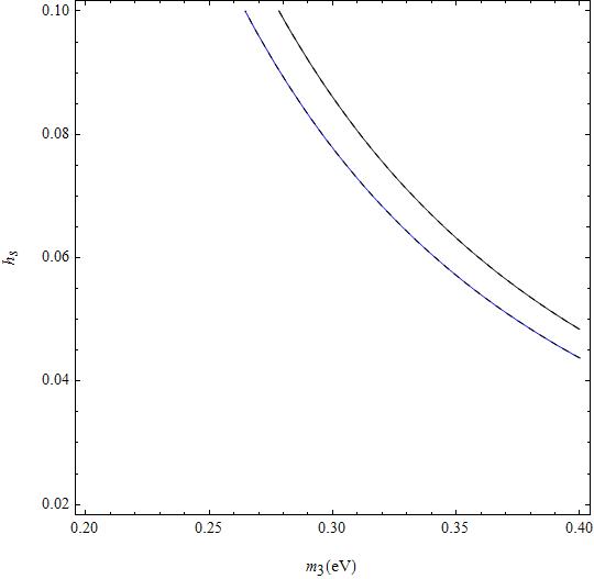
From Fig. 1, for $\sin\theta_{13}$ all the region below the curves is physically acceptable, within $1\sigma$ deviation. At the same time, one observes that the $\sin\theta_{13}$ allowed region is mostly insensitive to hierarchy, meaning, we can not differentiate between normal and inverted hierarchy. Indeed, the regions basically overlap, so that, both hierarchies share most of the same parameter region. In particular, two extreme points we have to comment on: for small values of $h_{s}$, $m_{3}$ is close to its maximal value. On the other hand, for large values of $h_{s}$, $m_{3}$ is larger than its middle maximal value. In addition, from the figure one may identify a window of acceptable values, which lies within $h_{s}\approx\left(0.04-0.1\right)$ and $m_{3}\approx\left(0.26-0.4\right)$. The important result here is that $h_{s}$ must be tiny in order to have a consistent value for $\sin\theta_{13}$, according to the experimental limits. The same conclusion will arise for $\sin\alpha$, as we will see from Fig. 2.

Figure 2: The $1\sigma$ region for $\sin\alpha$ as a function of $h_{s}$ and $m_{3}$, for both normal (solid line) and inverted (dashed line) hierarchies. The upper and lower contours correspond to the limit value of $\sin\alpha=0.07$.

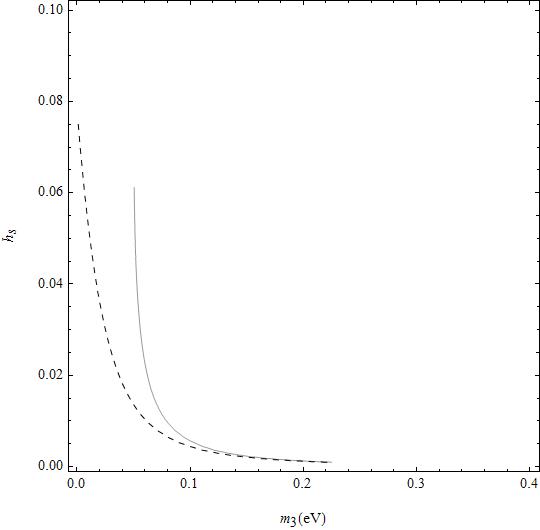
Before starting the discussion about Fig. 2, we would like to comment that we have taken the absolute value of $\sin\alpha$ just for the sake of depicting together all cases in the same plot. However, the case of inverted hierarchy produces negative values for $\sin\alpha$, which already introduces a way to distinguish the hierarchy if one could identify in what direction $\theta_{23}$ deviates from the maximal value. We also observe that normal and inverted hierarchy can easily differentiate at small values of $m_{3}$. However, for tiny values of $h_{s}$ (and large values for $m_{3}$) both of them are difficult to point out from each other (apart from the overall sign). This plot is more constrained since the allowed parameter region for $\sin\alpha$ remains below the contours for each hierarchy. Again, from this figure we infer the phenomenologically valid interval of values that gets within $h_{s}\approx\left(0.001-0.07\right)$ and $m_{3}\approx\left(0.001-0.22\right)$ for inverted hierarchy, and $h_{s}\approx\left(0.001-0.06\right)$ and $m_{3}\approx\left(0.06-0.22\right)$ for normal hierarchy. Comparing the parameter regions of $m_{3}$ for $\sin\theta_{13}$ and $\sin\alpha$ graphics, this seems to be in disagreement since both sets of values should be common in order to satisfy simultaneously such expressions. Nonetheless, in Fig. 3 we show the valid region of values for $m_{3}$ to both hierarchy cases.

One interesting prediction of the model is that the ratio $\sin\alpha/\sin\theta_{13}$ does not depend on the parameter $h_{s}$, as we already pointed out, and thus, an appealing formula arises which represents the key expression that allows one to falsify this model

$$\frac{\sin\alpha}{\sin\theta_{13}}\approx\left[\cot 2\theta_{\odot}+\frac{m^{2}_{3}-AB}{m_{3}\sin 2\theta_{\odot}(A-B)}\right],$$ (20)

This ratio is principally driven by the second term which has a clear dependence on $m_{3}$ and the rest of the observables, and also an extra contribution comes from the solar angle. This can be enhanced or decreased depending on the hierarchy scheme, in particular, for strict normal hierarchy one obtains a fit value of about $68.45$ when central values are taken for the observables. On the other hand, inverted hierarchy has a notable dependence on $m_{3}$ whose value is not well determined. One can in general depict the expected ratio in terms of $m_{3}$, as we show explicitly in Fig. 3.

Figure 3: The $1\sigma$ region for $|\sin\alpha|/\sin\theta_{13}$ as function of $m_{3}$, for both normal ( solid lines) and inverted ( dashed lines ) hierarchies.

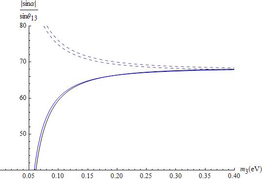
As we can see from Fig. 3, there is a clear difference between both hierarchies for small values of the $m_{3}$ mass scale. For normal hierarchy the ratio decreases with the hierarchy scale $m_{3}$, whereas for inverted hierarchy the ratio rather increases (negatively) with $m_{3}$. However, it is hard to differentiate between the two hierarchies for large $m_{3}$. The most important point we do want to make about this plot is that our model, under the previous approximations, predicts that due to the correlation between $|\sin\alpha|$ and $\sin\theta_{13}$, the latter parameter will very likely lie in below a range of $10^{-3}$, which can be difficult to reach in future experiments, given that $|\sin\alpha|\approx|\frac{1}{2}-\sin^{2}\theta_{23}|$ is already bounded below $10^{-2}$ by current experimental data. Nevertheless, this correlation will make it possible to falsify our model in the following way. If future experiments achieve to measure $|\sin\alpha|$ and/or $\sin\theta_{13}$, then, they should lie in the allowed region according to Fig. 3. On the contrary, if such were not the case, the model would be automatically discarded.

V CP phase contribution

Next, let us add some comments on CP phase contributions. As we already stated, and as we will discuss below, it seems unlikely that such contributions may drastically change our results. In particular, aside from some small numerical changes, it does appear yet difficult that CP phases may increase the tight upper bound the model indicates for $\sin\theta_{13}$, which has been put on at about $10^{-3}$, and which is already far away from the current experimental bound ($\sim 10^{-1}$).

In order to show our present point in a simple way, let us briefly reconsider our analysis of Sec. III. As usual, the mixing matrix is in general given by $U=U_{PMNS}K$, where $K=diag(1,e^{i\phi_{1}},e^{i\phi_{2}})$ stand for the Majorana CP phases. Also, $U_{PMNS}$ contains (in the standard parametrization) the $\varphi$ Dirac CP phase. So that, under the same considerations as for Sec. III, $M_{\nu}$ is diagonalized by $U$, and Eqs.(8-9) get replaced by

$$z = \frac{1}{\sqrt{2}}\left[\frac{P^{\ast}\left(\delta-\epsilon C\right)-K\left(\delta-\epsilon C\right)^{\ast}}{\mid P\mid^{2}-\mid K\mid^{2}}\right];$$ (21)

$$\sin\alpha = -\frac{1}{4m_{\mu\tau}}\left[\epsilon+\sqrt{8}z\overline{m}_{e\mu}\right]$$ (22)

where, as before, $z=\sin\theta_{13}e^{i\varphi}$, and we have introduced the short-hand notation where $P=\overline{m}^{2}_{e\mu}/m_{\mu\tau}-m_{ee}$, $K=\overline{m}_{\mu\mu}-m_{\mu\tau}$ and $C=\overline{m}_{e\mu}/2m_{\mu\tau}$. Here, $\delta$ and $\epsilon$ parameters have the same form as in previous sections. We must keep in mind the $M_{\nu}$ matrix elements are now complex ($\mid m_{\alpha\beta}\mid e^{i\rho_{j}}$, where $\alpha,\beta=e,\mu,\tau$, and $j=1,..,6$), and the Majorana CP phases are implicitly included in Eqs. (21-22). Of course, when CP phases are canceled (taking all masses to be real), the above expressions reduce to the previous results as given in Eqs. (8-9). Interesting enough, Eq. (7) maintains its form even in the presence of CP phases.

Having written the modified formulas for $\sin\theta_{13}$ and $\sin\alpha$, we are now interested in figuring out how CP-violating phases affect our previous considerations and conclusions. Performing a complete and general analysis of the CP-violating case is challenging and complicated. Nevertheless, there is a simpler way to proceed for our purpose, and that is to use the numerical results that came from our previous analysis as a grounding point, to estimate, through a general example, the effect of reintroducing non-trivial CP phases. Hence, we will proceed as follows: first, we use our CP-conserving results to rebuild the effective neutrino mass matrix elements, thus identified as $|m_{\alpha\beta}|$, for a given set of initial inputs, and then reintroducing CP phases on $M_{\nu}$, and recalculating our predictions to determine how far the new results are from those expected from the CP-conserving case. We will particularly focus on the correlation given in Eq. (20), which is our main result here. Moreover, since the absolute values of $\delta/m_{e\mu}$ and $\epsilon/m_{\mu\mu}$ are supposed to be small, we may conclude that $m_{e\mu}$ and $m_{e\tau}$ will have about the same phase, as so will $m_{\mu\mu}$ and $m_{\tau\tau}$, irrespective of $\delta$ and $\epsilon$ own arbitrary phases. For simplicity, we will suppose that $\overline{m}_{e\mu}$ and $\delta$ have the same phase, and analogously for $\overline{m}_{\mu\mu}$ and $\epsilon$; this choice shall reduce the number of CP phases on $M_{\nu}$ to four, although, it is clear not all will be truly physical. Under these considerations, the correlation between $\sin\alpha$ and $\sin\theta_{13}$ is now expressed as

$$\frac{|\sin\alpha|}{|z|}\approx\frac{1}{\sqrt{2}|m_{\mu\tau}m_{ee}|}\frac{\left||\overline{m}_{\mu\mu}|f_{1}e^{i\gamma_{1}}+|\overline{m}^{2}_{e\mu}|f_{2}\right|}{\mid f_{2}\mid}$$ (23)

where we have defined

$$f_{1} = \left||\overline{m}^{2}_{e\mu}|-|m_{\mu\tau}m_{ee}|e^{i\gamma}\right|^{2}$$ (24)

$$-\mid m_{\mu\tau}^{2}\mid\left||\overline{m}_{\mu\mu}|e^{i\gamma_{1}}-|m_{\mu\tau}|\right|^{2};$$

and

$$f_{2} = \left[|\overline{m}_{e\mu}^{2}|-|m_{\mu\tau}m_{ee}|e^{-i\gamma}+|m_{\mu\tau}^{2}|-|m_{\mu\tau}\overline{m}_{\mu\mu}|e^{-i\gamma_{1}}\right]$$ (25)

$$\times\left(|m_{\mu\tau}|-|\overline{m}_{\mu\mu}|e^{i\gamma_{1}}\right).$$

Here, $\gamma=\rho_{1}+\rho_{3}-2\rho_{2}$ and $\gamma_{1}=\rho_{4}-\rho_{3}$ stand for the two effective CP-violating phases entering in our results that came out of combinations of the arbitrary phases we first introduced in the neutrino mass matrix. Therefore, we realize the correlation among mixings depends only on these two CP phases, apart from the $m_{3}$ hierarchy mass scale.

Next, we can use Eq. (23) to quantify the phase dependence of our previous CP invariant results. This we do by exploring some general examples, by taking specific values for $\gamma$ and $\gamma_{1}$, and then replotting the ratio $|\sin\alpha|/|z|$ as functions of $m_{3}$ for the central values of the observables. We show in Fig 4 (solid line) the results we obtained for the CP invariant case, that is for $\gamma=0$ and $\gamma_{1}=0$, for both neutrino mass hierarchies, as before (see figure 3 for a comparison). Next, in same figure, short-dashed lines have been obtained when the arbitrary values $\gamma=\pi/4$ and $\gamma_{1}=\pi/5$ are taken. Similarly, for $\gamma=\pi/2$ and $\gamma_{1}=\pi/4$ the associated plot is represented by the dotted line. Finally, the long-dashed line stands for the arbitrary set of values $\gamma=\pi/7$ and $\gamma_{1}=\pi/2$.

Figure 4: Upper bound for $|\sin\alpha|/|z|$ as a function of $m_{3}$, for different values of $\gamma$ and $\gamma_{1}$ as discussed in the text. As before, for normal hierarchy, the contours (the correlation) decrease for small values of $m_{3}$ whereas for inverted hierarchy the contours increase (negatively).

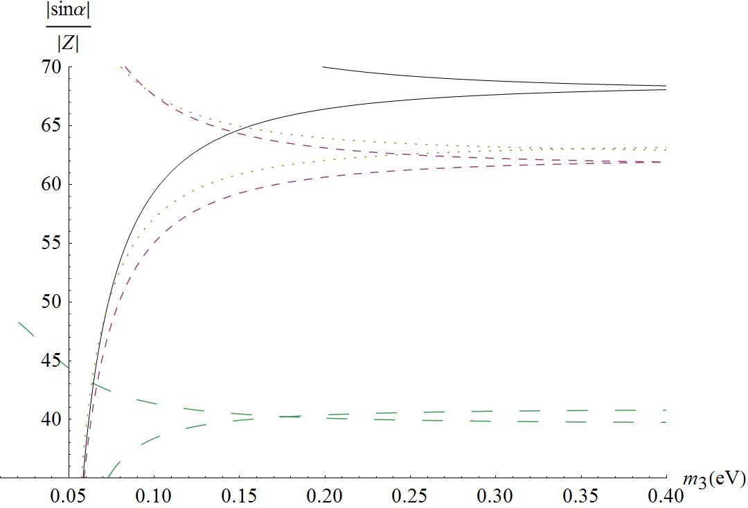
From Fig. (4), one may deduce important facts about the CP- violating phases contributions to the correlation between $\sin\alpha$ and $\sin\theta_{13}$: In general, for both hierarchies, CP phases do not change the general profile of the $1\sigma$ regions, and neither seem to introduce drastic changes on the $\sin\alpha/\sin\theta_{13}$ ratio, which at least for the arbitrary values we have explored, keeps $\sin\theta_{13}$ upper bound on about $10^{-3}$, as we have pointed out before. Indeed, in spite of considering the largest changes we found on the mixing correlation (for $\gamma=\pi/7$ and $\gamma_{1}=\pi/2$), the result is not yet enough to significantly reduce the bound.

Nonetheless, as a cautionary word, as we have not presented here a truly general analysis for the CP-violating case, we can not discard the possibility that CP phases may conspire among themselves to produce an accidental enhancement of the $\sin\alpha/\sin\theta_{13}$ ratio. A naive analysis shows that this seems to happen for instance for the precise values of $\gamma=\pi$ and $\gamma_{1}=\pi$, which set the mentioned ratio to the order of $10^{-1}$, which in turn would locate $\sin\theta_{13}$ close to the experimental sensitivity level. However, such a case has almost no parameter space on the CP phase sector, and it seems very unlikely that such extreme values could be potentially physical, since even phases are subject to higher order corrections, and no symmetry exists that may protect phases as to keep them at those precise values. Thus, a conservative point of view would point towards the strength of our previous CP invariant results. A more careful and general study of CP violation in $\mu\leftrightarrow\tau$ symmetric models is in progress, and a detailed analysis of this scenario will be presented soon elsewhere.

VI Conclusions

We studied the lepton sector of the LRSM dressed with a $(Z_{2})^{3}$ discrete symmetry, as was done in two frameworks: (1) neglecting the CP- violating phases and (2) involving them. Using discrete symmetries we build a framework where the charged lepton mass matrix is diagonal at tree level, so that we start since the beginning in the true flavor basis, and get a model that naturally realizes a slightly broken $\mu\leftrightarrow\tau$ symmetry. In addition, we have determined $\theta_{13}$ and the deviation from the maximal value of $\theta_{23}$ in the limit of a small $\mu\leftrightarrow\tau$ symmetry breaking that appears at tree level in the effective neutrino mass matrix. These two expressions are fixed in terms of one free parameter of the model, $h_{s}$, the mass scale hierarchy $m_{3}$ (for the first scenario), and two CP-violating phases (for the second one); within the first scenario, a set of values for $h_{s}$ and $m_{3}$ were found which are consistent with current limits imposed by the experimental data for $\sin\theta_{23}$ and $\sin\theta_{13}$.

The present model is quite elaborate, but predictive. In particular, a correlation among $\sin\alpha$ that measures the deviation of $\sin^{2}\theta_{23}$ from $1/2$, and $\sin\theta_{13}$ arises which only depends on one neutrino mass scale, $m_{3}$ (and the CP phases). This is a remarkable result and provides a way to test the model, since the observed value of $|\sin\alpha|/\sin\theta_{13}$ would also provide a direct determination of the scale of $m_{3}$ for a given hierarchy. We should point out this ratio does predict an allowed region for $\sin\theta_{13}$ which must be below $10^{-3}$, in order to satisfy the current experimental data, that upper bounds the expression $1/2-\sin^{2}\theta_{23}$. Such a sensitivity could be hard to reach in future experiments but it seems possible. On the other hand, as an extra bonus of this model, a clear determination of the $m_{ee}$ strength of double beta decay was found.

VII appendix

The most general form of the scalar potential of the LRSM was analyzed in boris , and it has 18 terms which are invariant under the gauge group $SU(2)_{L}\times SU(2)_{R}\times U(1)_{B-L}$ and parity. Now, from our scalar particle content: two bidoublets $\phi_{i}$ ($i=1,2$), and four triplets, $\Delta_{j}$ ($j=1,...,4$), we should write the potential. Even though, it is larger than the original potential, it is possible to show by a lengthy calculation that it has a least a minimum. Here we are interested in showing that the triplets $\Delta_{2R}$ and $\Delta_{3R}$ have the same VEV when we minimize the potential. So, without loss of generality, we just write the terms in which their VEV’-s are involved after spontaneous symmetry breaking and they are given as:

$$V = \left(v_{2R}^{2}+v_{3R}^{2}\right)\bigg{[}-\mu_{1}^{2}+2bv_{1R}^{2}+2b_{1}v_{4R}^{2}+4b_{3}k_{1}k_{1}^{{}^{\prime}}$$ (26)

$$+b_{2}\left(k_{1}^{2}+k_{1}^{{}^{\prime}2}\right)+b_{4}k_{1}^{{}^{\prime}2}+b_{5}\left(k_{2}^{2}+k_{2}^{{}^{\prime}2}\right)+4b_{6}k_{2}k_{2}^{{}^{\prime}}$$

$$+b_{7}k_{2}^{{}^{\prime}2}\bigg{]}+b_{8}\left(v_{2R}^{4}+v_{3R}^{4}\right)+2b_{9}v_{2R}^{2}v_{3R}^{2}+...$$

We can easily conclude from the above expression that $\Delta_{2R}$ and $\Delta_{3R}$ have the same VEV, by directly calculating the two minimization conditions, $\frac{\partial V}{\partial v_{2R}}=\frac{\partial V}{\partial v_{2R}}=0$. It is not difficult to realize that this is a consequence of the fact that $V$ remains symmetric under the $v_{2R}\leftrightarrow v_{3R}$ exchange, derived from the original $Z_{2}$ symmetry. This ensures that the Majorana mass matrix, $M_{R}$, will remain invariant under $\mu\leftrightarrow\tau$ symmetry after spontaneous symmetry breaking. On the other hand, we have to keep in mind that all VEV’-s will only depend on potential parameters after solving the simultaneous conditions for each VEV.

References

- (1) Z. Maki, M. Nakagawa, S. Sakata, Prog. Theor. Phys. 28, 870 (1962); B. Pontecorvo, Zh. Eksp. Teor. Fiz. 53, 1717 (1968) [Sov. Phys. JETP 26, 984 (1968)].
- (2) Tomas Schwetz, Mariam Tórtola, and José W. F. Valle, New J. Phys.10, 113011 (2008).
- (3) M.C. Gonzales-Garcia and M. Maltoni, Proc. Sci., idm2008 (2008) 072.
- (4) K. Anderson et al., hep-ex/0402041; F. Ardellier, et al. (Double Chooz Collaboration), hep-ex/0606025; A. B. Balantekin , et al. (Daya Bay Collaboration), hep-ex/0701029; Y. Itow, et al. (T2K Collaboration), hep-ex/0106019; D. S. Ayres et al. (NOvA Collaboration), hep-ex/0503053; D. G. Michael et al. (MINOS Collaboration), Phys. Rev. Lett. 97, 191801 (2006).
- (5) M. Gell-Mann, P. Ramond, R. Slansky, in Supergravity, edited by D. Freedman and P. van Nieuwenhuizen (North-Holland, Amsterdam, 1979) p. 315; T. Yanagida, in Proceedings of the Workshop on Unified Theory and Baryon Number in the Universe, edited by O. Sawada and A. Sugamoto (KEK, Tsukuba, Japan, 1979) p. 95; R.N. Mohapatra, G. Senjanovic, Phys. Rev. Lett. 44, 912 (1980); idem Phys. Rev. D23, 165 (1981); P. Minkowski, Phys. Lett. B67, 421 (1977).
- (6) J. C. Pati and A. Salam, Phys. Rev. D10, 275(1974); R. N. Mohapatra and J. C. Pati, Phys. Rev. D 11, 566 (1975); 11, 2558 (1975); G. Sejanovic and R. N. Mohapatra, Phys. Rev. D 12, 1502 (1975).
- (7) R.N. Mohapatra, S. Nussinov, Phys. Rev. D60, 013002 (1999); C.S. Lam, Phys. Lett. B507, 214 (2001); T. Kitabayashi, M. Yasue, Phys. Rev. D67, 015006 (2003); W. Grimus, L. Lavoura, Phys. Lett. B572, 189 (2003); Y. Koide, Phys. Rev. D69, 093001 (2004); T. Fukuyama, H. Nishiura, hep-ph/9702253.
- (8) Juan Carlos Gómez-Izquierdo, Abdel Pérez-Lorenzana,Phys. Rev. D77, 113015 (2008).
- (9) N. G. Deshpande et al., Phys. Rev. D44, 837 (1991).
- (10) R. N. Mohapatra, S. Nussinov, Phys. Lett. B441, 299 (1998).
- (11) For an incomplete list, see for instance: P. F. Harrison, W. G. Scott, Phys. Lett.B547, 219 (2002); R. N. Mohapatra, J. High Energy Phys. 10, 027 (2004); R. N. Mohapatra, S. Nasri, H.-B. Yu, Phys. Lett. B636, 114 (2006); A. S. Joshipura, Eur.Phys. J. C 53, 77 (2007); E. Ma, Phys. Rev. D70, 031901(R) (2004); K. S. Babu, R. N. Mohapatra, Phys. Lett. B532, 77 (2002); K. Fuki, M. Yasue, Nucl. Phys. B 783,31 (2007); A. Goshal, Mod. Phys. Lett. A19, 2579 (2004); T. Ohlsson, G. Seidl, Nucl. Phys. B643, 247(2002); Riazuddin, Eur. Phys. J. C51, 697 (2007); Y. Koide, E. Takasugi, Phys. Rev. D 77, 016006 (2008); C. Luhn et al., Phys. Lett. B652, 27 (2007); M. Honda, M. Tanimoto, Prog. Theor. Phys. 119 (2008) 583; H.Ishimori et al., Phys. Lett. B662, 178 (2008).
- (12) Walter Grimus and Luís Lavoura, Phys. Lett. B572, 189 (2003); J. High Energy Phys. 07 (2004) 45.