Abstract

We present the consequences of a large radiative correction term coming from Supersymmetry (SUSY) upon the electron neutrino fluxes streaming off a core-collapse supernova using a 3-flavour neutrino-neutrino interaction code. We explore the interplay between the neutrino-neutrino interaction and the effects of the resonance associated with the $\mu-\tau$ neutrino index of refraction. We find that sizeable effects may be visible in the flux on Earth and, consequently, on the number of events upon the energy signal of electron neutrinos in a liquid argon detector. Such effects could lead to a probe for Beyond Standard Model (BSM) physics and, ideally, to constraints in the SUSY parameter space.

LPT Orsay 10-13

1 Introduction

During the past decade, our comprehension of the neutrino interactions in a supernova environment has deeply evolved, due to the increasing precision of neutrino experiments and computational force. In addition with the traditional MSW effect  [1, 2], the neutrino-neutrino interaction has been proven to be fundamental for the neutrino evolution in such environment. This interaction, whose effects have changed the existing paradigm of SN neutrino physics, has been recently the subject of intense investigation [3, 4, 5, 6, 7, 8, 9, 10, 11, 12, 13, 14, 15, 16, 17, 18, 19, 20, 21]. For a recent extensive review on this subject, see [22].

In addition with these interactions, an other matter interaction $V_{\mu\tau}$, which arises at one-loop order ($O\left({\alpha\over\pi\sin^{2}\theta_{W}}{m_{\tau}^{2}\over M_{W}^{2}}\right)$) makes the mu and tau neutrino index of refraction different [23, 24]. This radiative correction potential is related to the charged-current matter potential $V_{c}$, in an electrically neutral medium, by a parameter $\varepsilon$, which is defined as $-p_{\nu}\Delta n_{\tau\mu}=V_{\mu\tau}=\varepsilon V_{e}$. The value of $\varepsilon$ is $5.4\times\,10^{-5}$ in the Standard Model. Only a few papers have shown the interest of such radiative correction term. Without the neutrino-neutrino interaction, $V_{\mu\tau}$ has been shown to present effects on Earth if the $\nu_{\mu}$ and $\nu_{\tau}$ fluxes are different at emission [25]. Via a non-zero CP-violating phase, $V_{\mu\tau}$ can also in theory induce effects on the (anti-) electron neutrino fluxes in the Sun [26] or in a supernova environment [27, 28]. Including the collective effects, the CP-violation effects due to $V_{\mu\tau}$ turn out to be larger [29], and the electron neutrino flux displays a $\theta_{23}$ dependence in presence of a large $V_{\mu\tau}$ coming from a high density profile [30, 31].

Despite its success, the Standard Model (SM) of particle physics exhibits a number of shortcomings which might be remedied by new Physics showing up at the Terascale. One very popular extension of the SM is Supersymmetry (SUSY) [32]. Virtues of SUSY are numerous: it can provide a natural candidate to explain dark matter and it allows the elimination of the hierarchy problem and the unification of the gauge couplings at the scale of grand unification ($M_{GUT}$).

In a previous paper, we have calculated all one-loop radiative correction terms to the matter interaction in the SUSY framework [33]. SUSY particles like sleptons, squarks up and down, charged Higgs, neutralinos and charginos take place in these loops. With a dedicated numerical routine, we have scanned and identified regions in the parameter space that yield interesting value of the $V_{\mu\tau}$ potential, namely large values up to $\varepsilon_{SUSY}\simeq 2.10^{-2}$.

The recent simulations of neutrino evolution [34, 35] in supernova take into account a dynamical density profile, in addition with the neutrino collective effects. All interactions combined show a characteristic imprint in the anti-neutrino fluxes, whose detection could yield precious information concerning the dynamics of the density profile or fundamental neutrinos properties like the hierarchy or the value of the third mixing angle $\theta_{13}$. With larger value of $\varepsilon$ than in the SM case, we show that $V_{\mu\tau}$ can exhibit sizeable and characteristic effects on the electron neutrino fluxes particularly in the inverse hierarchy where the $\nu-\nu$ interaction display salient features such as the synchronization regime, the bipolar transition and the spectral split. Such BSM imprints could be seen in a neutrino observatory on Earth and could ideally lead to constraints in the SUSY parameter space.

The paper is organized as follows. In Sec. 2 we explicit the evolution equations which lead to the calculation of the electron neutrino flux, describe the framework used, and justify the approximations taken to yield our results. In Sec. 3 we describe the three typical behaviours that can occur due to the interplay between the neutrino-neutrino interaction and the $\mu-\tau$ resonance. In Sec. 4 and Sec. 5, we analyze the role of the parameters that can influence such interplay and consequently the $\nu_{e}$ flux as a function of energy. The subsections 5.2 and 5.3 are dedicated to the study of the consequence of varying the luminosity and the density which is equivalent to looking at the flux at different times. We then use these fluxes to display the number of events in a liquid argon detector that we describe in Sec. 6. Finally, before concluding in Sec. 8, we discuss in Sec. 7, about the possibility of the observation of such beyond standard effects for realistic conditions.

2 Theoretical framework

The main goal of this paper is to explore the impacts of the parameters that influence the interplay between the neutrino-neutrino interaction and the $\mu-\tau$ resonance and consequently study the possibility that such effects can be observable in a neutrino observatory in order to get a possible probe for models BSM. In this section, we first present the evolution equation we have numerically solved and the hypothesis used to yield the results of the following sections.

2.1 Equation of evolution.

In a dense environment the non-linear coupled neutrino evolution equations with neutrino self-interactions are given by:

$$i{d\over{dt}}\psi_{{\nu}_{\underline{\alpha}}}=[H_{0}+H_{m}+H_{\nu\nu}]\psi_{{\nu}_{\underline{\alpha}}}$$ (1)

where $\psi_{{\nu}_{\underline{\alpha}}}$ denotes a neutrino created at the neutrinosphere initially in a flavour state $\alpha=e,\mu,\tau$, $H_{0}=UH_{vac}U^{\dagger}$ is the Hamiltonian describing the vacuum oscillations $H_{vac}=\mathrm{diag}(E_{1},E_{2},E_{3})$, $E_{i=1,2,3}$ being the energies of the neutrino mass eigenstates, and $U$ the unitary Maki-Nakagawa-Sakata-Pontecorvo matrix

$$U=T_{23}T_{13}T_{12}=\left(\matrix{1&0&0\cr 0&c_{23}&s_{23}\cr 0&-s_{23}&c_{23}}\right)\left(\matrix{c_{13}&0&s_{13}e^{-i\delta}\cr 0&1&0\cr-s_{13}e^{i\delta}&0&c_{13}}\right)\left(\matrix{c_{12}&s_{12}&0\cr-s_{12}&c_{12}&0\cr 0&0&1}\right),$$ (2)

$c_{ij}=\cos\theta_{ij}$ ($s_{ij}=\sin\theta_{ij}$) with $\theta_{12},\theta_{23}$ and $\theta_{13}$ the three neutrino mixing angles. The presence of a Dirac $\delta$ phase in Eq.(2) renders $U$ complex and introduces a difference between matter and anti-matter.

The neutrino interaction with matter is taken into account through an effective Hamiltonian which corresponds to the diagonal matrix $H_{m}=diag(V_{e},0,V_{\mu\tau})$. $V_{e}(r)=\sqrt{2}G_{F}n_{e}(r)$ is the matter potential due to the charged-current interaction between electron (anti-) neutrinos and the electrons present in the medium where $G_{F}$ is the Fermi coupling constant and $n_{e}(r)$ is the electron density in the star. At the tree level, neutral current interactions introduce an overall phase only. Note that this density will imply in supernova possibly two resonances when the MSW condition [2] (here shown for two flavours) is reached:

$$\frac{\Delta m^{2}}{2E_{\nu}}\cos 2\theta=V_{e}(r)$$ (3)

Depending on the sign of $\Delta m_{32}^{2}$ ,the ”H-resonance” (high density) may happen either for neutrinos or anti-neutrinos while the ”L-resonance” (low density) happens for neutrinos only and is dependent on $\Delta m_{21}^{2}$.

As previously mentioned, in the Standard Model case, Botella et al. in [23] have highlighted the presence of a one-loop matter potential arising from radiative corrections to neutral-current $\nu_{\mu}$ and $\nu_{\tau}$ scattering. Such matter potential can therefore be seen as an effective presence of $\tau$ particles and one can write

$$V_{\mu\tau}=\sqrt{2}\,G_{\rm F}Y_{\tau,SM}^{\rm eff}n_{B}$$ (4)

where $n_{B}$ is the baryon density inside the supernova and

$$Y_{\tau,SM}^{\rm eff}=\frac{3\sqrt{2}\,G_{\rm F}m_{\tau}^{2}}{(2\pi)^{2}}\left[\ln\left(\frac{m_{W}^{2}}{m_{\tau}^{2}}\right)-1+\frac{Y_{n}}{3}\right]=2.7\times 10^{-5}\,,$$ (5)

The value of $Y_{\tau,SM}^{\rm eff}$ is obtained using the hypothesis of a isoscalar medium i.e, $n_{e}=n_{p}=n_{n}$ ($n_{p}$ and $n_{n}$ being respectively the proton and neutron density in the star), therefore the neutron fraction $Y_{n}=n_{n}/(n_{p}+n_{n})$ is equal to 0.5. For our convenience, we have defined the overall radiative correction factor as :

$$\varepsilon=\frac{Y_{\tau,SM}^{\rm eff}+Y_{\tau,SUSY}^{\rm eff}}{Y_{e}}$$ (6)

where $Y_{\tau,SUSY}^{\rm eff}=0$ in the Standard Model and the electron fraction $Y_{e}=n_{e}/(n_{n}+n_{p})$ is taken to be 0.5 all along the paper.

The general form of the neutrino self-interaction term is

$$H_{\nu\nu}=\sqrt{2}G_{F}\sum_{\alpha}\sum_{\nu_{\alpha},\bar{\nu}_{\alpha}}\int\rho_{{\nu}_{\underline{\alpha}}}({\bf q}^{\prime})(1-{\bf\hat{q}}\cdot{\bf\hat{q}^{\prime}})dn_{\alpha}dq^{\prime}$$ (7)

where $\rho=\rho_{{\nu}_{\underline{\alpha}}}$ ($-\rho^{*}_{{\nu}_{\underline{\alpha}}}$) is the density matrix for neutrinos (antineutrinos)

$$\rho_{{\nu}_{\underline{\alpha}}}=\left(\matrix{|\psi_{\nu_{e}}|^{2}&\psi_{\nu_{e}}\psi_{\nu_{\mu}}^{*}&\psi_{\nu_{e}}\psi_{\nu_{\tau}}^{*}\cr\psi_{\nu_{e}}^{*}\psi_{\nu_{\mu}}&|\psi_{\nu_{\mu}}|^{2}&\psi_{\nu_{\mu}}\psi_{\nu_{\tau}}^{*}\cr\psi_{\nu_{e}}^{*}\psi_{\nu_{\tau}}&\psi_{\nu_{\mu}}^{*}\psi_{\nu_{\tau}}&|\psi_{\nu_{\tau}}|^{2}}\right),$$ (8)

${\bf q}$ (${\bf q^{\prime}}$) denotes the momentum of the neutrino of interest (background neutrino) and $dn_{\alpha}$ is the differential number density. The emission geometry is based on the so called “bulb model” with spherical symmetry [12]: neutrinos are assumed to be half-isotropically emitted from the neutrinosphere.

In the multi-angle treatment, SN neutrinos travel on different trajectories. This is taken into account by the factor $(1-{\bf\hat{q}}\cdot{\bf\hat{q}^{\prime}})$ in Eq.(7). The single angle approximation consists of averaging such factor along the polar axis, i.e. $\rho({\bf q})=\rho(q)$, Eq.(7) reduces to

$$H_{\nu\nu}={\sqrt{2}G_{F}\over{2\pi R_{\nu}^{2}}}D(r/R_{\nu})\sum_{\alpha}\int[\rho_{{\nu}_{\underline{\alpha}}}(q^{\prime})L_{{\nu}_{\underline{\alpha}}}(q^{\prime})-\rho_{\bar{{\nu}}_{\underline{\alpha}}}^{*}(q^{\prime})L_{\bar{{\nu}}_{\underline{\alpha}}}(q^{\prime})]dq^{\prime}$$ (9)

with the geometrical factor

$$D(r/R)={1\over 2}\left[1-\sqrt{1-\left({R\over r}\right)^{2}}\right]^{2}$$ (10)

where the radius of the neutrino sphere is $R=10$km. In a spherically symmetric environment, a single-angle treatment tends to capture the main non-linear behaviour.

For this paper, we shall adopt

$$L_{{\nu}_{\underline{\alpha}}}(E_{\nu})={L^{0}_{{\nu}_{\underline{\alpha}}}\over{T_{\nu_{\underline{\alpha}}}^{3}\langle E_{\nu_{\underline{\alpha}}}\rangle F_{2}(\eta)}}{{E_{\nu_{\underline{\alpha}}}^{2}}\over{1+\exp{(E_{\nu_{\underline{\alpha}}}/T_{\nu_{\underline{\alpha}}}-\eta)}}}$$ (11)

as the neutrino luminosity, where $F_{2}(\eta)$ is the Fermi integral, $L^{0}_{{\nu}_{\underline{\alpha}}}$ and $T_{\nu_{\underline{\alpha}}}$ are the luminosity and temperature at the neutrinosphere. $\langle E_{\nu_{\underline{\alpha}}}\rangle$ is the average neutrino energy of the corresponding flavour $\alpha$.

As we are going to see in the following sections, the neutrino-neutrino interaction is characterized by three distinct phases for the neutrino evolution: the synchronization regime, the bipolar transition and the spectral split. The synchronized regime takes place in the first 50 km outside the neutrino sphere. In this phase, the strong neutrino-neutrino interaction makes neutrinos of all energies oscillate with the same frequency so that flavour conversion is frozen [8, 15]. When the neutrino self-interaction term diminishes, large bipolar oscillations appear that produce strong flavour conversion for both neutrinos and anti-neutrinos for the case of inverted hierarchy, as long as the $\theta_{13}$ value [13] is non-zero. Eventually neutrinos show complete (no) flavour conversion for energies larger (smaller) than a characteristic energy $E_{c}\simeq 8$MeV which can be related to the lepton number conservation [17]. This is the spectral split phenomenon: while electron neutrinos swap their spectra with muon and tau neutrinos; the electron anti-neutrinos show a complete spectral swapping. Such behaviours are found for both large and small values of the third neutrino mixing angle, contrary to the standard MSW effect.

We have chosen here to describe the evolution equation using wave-functions such as in [12, 29] for instance. Note that equivalently the density matrix or the polarization vector formalism can be used to describe the neutrino evolution in the supernova environment.

2.2 Work hypothesis.

We give the general framework and the hypothesis that we make to obtain our numerical results.

The results we obtained use the best fit oscillation parameters to date, i.e. $\Delta m^{2}_{21}=7.6\times 10^{-5}$eV², sin${}^{2}2\theta_{12}=0.87$ and $\mid\Delta m^{2}_{32}\mid=\mid\Delta m^{2}_{atm}\mid=2.43\times 10^{-3}$eV² for the solar and atmospheric differences of the mass squares and mixings, respectively [36]. Apart from Sec. 5.1, we choose $\theta_{23}=40^{\circ}$ in the first octant, i.e equivalent to $\sin^{2}2\theta_{23}=0.97$. Unless notified, the Dirac phase is taken to be zero and $\sin^{2}2\theta_{13}=0.1$. This value of $\theta_{13}$ taken is in agreement with the current experimental upper-limit [36].

During a supernova explosion, three distinct phases take place: the prompt deleptonization burst, the accretion phase, and the cooling phase. In this paper, we will focus on the neutrino signal produced during the early cooling phase where the density of neutrinos is sufficiently important to induce sizeable non-linear behaviour. Concerning the cooling phase, the hypothesis of equal luminosities and equipartition of energies among all neutrino flavours at the neutrino-sphere is made for the neutrino signal upon which we are focusing. We also make the assumption of an exponential decrease of the luminosity

$$L_{\nu}=L_{\nu,0}\times\exp(-t/\tau)$$ (12)

with $L_{\nu_{0}}=10^{52}$ erg $\cdot$ s^-1 and $\tau=3.5$ s the typical cooling time. Apart from Sec. 5.2 and Sec. 6, we look at time $t\simeq 8$s after post-bounce which corresponds to $L_{\nu}=10^{51}$ erg $\cdot$ s^-1 . We consider the hierarchy i.e. $\langle E_{\nu_{e}}\rangle<\langle E_{\bar{\nu}_{e}}\rangle<\langle E_{\nu_{x}}\rangle$ with typical values of 10, 15 and 24 MeV respectively. These values correspond approximatively to the cooling case I in [37].

In this paper, one of the observables is the $\nu_{e}$ flux, which can be written

$$\Phi_{\nu_{e}} = P(\nu_{e}\rightarrow\nu_{e})F^{R}_{\nu_{e}}+P(\nu_{e}\rightarrow\nu_{\mu})F^{R}_{\nu_{\mu}}+P(\nu_{e}\rightarrow\nu_{\tau})F^{R}_{\nu_{\tau}}$$ (13)

$$= P(\nu_{e}\rightarrow\nu_{e})(F^{R}_{\nu_{e}}-F^{R}_{\nu_{\mu}})+F^{R}_{\nu_{\mu}}$$

using the unitarity of the evolution operator of Eq.(1) and where $F^{R}_{\nu_{\alpha}}$ is the flux of flavour $\alpha$ emitted initially. We here made the hypothesis of equal $\nu_{\mu}$ and $\nu_{\tau}$ initial fluxes. We can link it to the luminosity $L_{{\nu}_{\underline{\alpha}}}(E_{\nu})$ defined in Eq.(11) via the relation:

$$F^{R}_{\nu_{\alpha}}=\frac{1}{4\pi R^{2}}L_{{\nu}_{\underline{\alpha}}}(E_{\nu})$$ (14)

Moreover, we define the flux received on Earth by

$$\Phi^{Earth}_{\nu_{e}}=<\Phi_{\nu_{e}}>=<P(\nu_{e}\rightarrow\nu_{e})>_{\rm{exit}}(F^{R}_{\nu_{e}}-F^{R}_{\nu_{\mu}})+F^{R}_{\nu_{\mu}}$$ (15)

The probability exiting the SN $<P(\nu_{e}\rightarrow\nu_{e})>_{\rm{exit}}$, and therefore the flux on Earth, is averaged over distance because of the decoherence phenomenon that takes place for neutrinos travelling over large distance in vacuum [38]. As the neutrinos stream off the supernova, a shock wave propagates through the SN envelope coming with a reverse shock. This induces a dynamical density profile which leads to the breaking of the adiabaticity of the H-resonance and possibly to a multiple resonance effect. Such interplay with the neutrino fluxes may imply a salient fingerprint on the signal received in an observatory on Earth as pointed out in [39, 40, 41, 34].

All along the paper we will focus on the electron neutrino flux in the inverted hierarchy. Consequently, the shock-wave effect should not impact on the electron neutrino flux since no H-resonance occurs. Therefore, for our electron number density, we adopt the usual simple analytical profile for the :

$$\lambda(r)=\sqrt{2}G_{F}n_{B}=\lambda_{r}\,\left(\frac{R}{r}\right)^{3}\,.$$ (16)

where R is equal to $10$km. Apart from Sec. 5.3 and Sec. 6, we take for reference $\lambda_{r}=5.7\times 10^{5}$km^-1 which corresponds to a late time density profile.

In [42], SM one-loop corrections to $\nu-\nu$ interaction have been studied and turned out to be of the same order as $Y_{\tau,SM}^{\rm eff}$ or even smaller. Though they have not been calculated yet, supersymmetric one-loop corrections to $\nu-\nu$ interaction will be similar to the SM ones but only larger in the same way than for $Y_{\tau,SUSY}^{\rm eff}$ in comparison with $Y_{\tau,SM}^{\rm eff}$. For $\varepsilon\lesssim 2.10^{-2}$, we expect them to be negligible. All the hypothesis made in this section will be discussed in Sec. 7.

3 Typical behaviour of a large $\mu$-$\tau$ radiative correction

In this section we review the consequences of a large $V_{\mu\tau}$ on the $\nu_{e}$ flux in the inverted hierarchy, in presence of the neutrino-neutrino interaction. Unlike in [30], we do not increase the value of the density $\lambda_{r}$ to obtain a large effective $\tau$ matter potential but we use instead the radiative correction term $\varepsilon$ whose value can rise depending on the SUSY parameters [33]. Consequently, varying the $\varepsilon$ for a given energy will only move the $\mu-\tau$ resonance above the synchronized region leaving unchanged the position of the L-resonance.

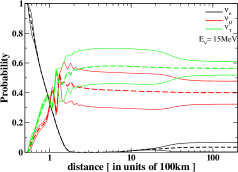
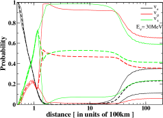
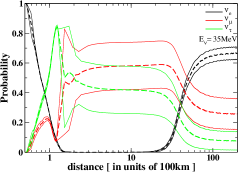
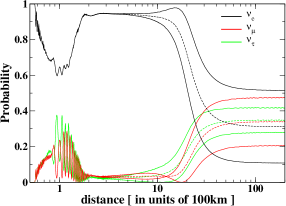
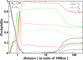
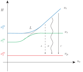
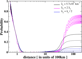
In Fig.(1) we show the oscillation probabilities for three different energies $E_{\nu}=15$, $30$ and $35$ MeV with $\varepsilon=\varepsilon_{r}=10^{-3}$ in order to identify precisely the physical effects appearing. Analogously to the $H$- and $L$-resonances, the radius where

$$r_{\mu\tau}=\left(\frac{\varepsilon 2E_{\nu}\sqrt{2}G_{F}Y_{e}\lambda_{r}}{\Delta m^{2}_{atm}}\right)^{1/3}R$$ (17)

defines approximatively the $\mu\tau$-resonance [25]. We also define here

$$\Delta r_{\mu\tau}=\tan 2\theta_{23}\left|\frac{V_{\mu\tau}^{\prime}}{V_{\mu\tau}}\right|^{-1}_{r=r_{\mu\tau}}\propto\tan 2\theta_{23}r_{\mu\tau}$$ (18)

as the resonance width, i.e the position around $r_{\mu\tau}$ where the $\mu-\tau$ resonance effects take place.

In [44], it has been shown that in the single angle approximation the neutrino-neutrino interaction term can be written as

$$\mu(r)=\mu_{0}\frac{R^{4}}{r^{4}}\frac{1}{2-R^{2}/r^{2}}$$ (19)

where

$$\mu_{0}=\sqrt{2}G_{F}(F^{R}_{\bar{\nu}_{e}}-F^{R}_{\bar{\nu}_{x}})$$ (20)

The bipolar transition starts when the synchronization ends ($r=r_{syn}$), and finish itself at $r_{bip}$ defined in [13] by the relation:

$$\mu(r_{bip})\simeq\frac{|\Delta m^{2}_{atm}|}{2E_{\nu}}.$$ (21)

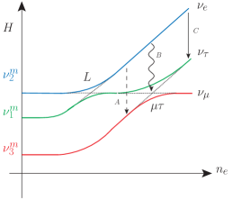
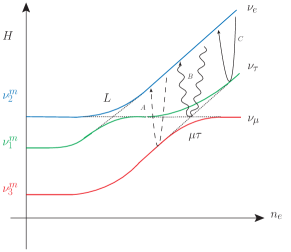
On the left panel of Fig.(1), for $E_{\nu}=15$ MeV, the $\mu-\tau$ resonance occurs before the bipolar transition ($r_{\mu\tau}+\frac{\Delta r_{\mu\tau}}{2}<r_{bip}$). Consequently, the matter eigenstates $\nu_{1}^{m}$ and $\nu_{3}^{m}$ start initially as a mix of $\nu_{\mu}$ and $\nu_{\tau}$. As can be seen in Fig.(2), in this case the collective effects (represented by an arrow with a dashed line) will lead to $\nu_{e}\approx\nu_{3}^{m}$ where $\nu_{3}^{m}$ is, at this moment, a mix of $\nu_{\mu}$ and $\nu_{\tau}$. We call this type of behaviour for the parameters $(\lambda_{r},\varepsilon)$ type A, it is equivalent to what happens in region III in [45]. In this region, as in the Standard Model case, the exact place where the L-resonance occurs does not really modify the value of $<P(\nu_{e}\rightarrow\nu_{e})>_{\rm{exit}}$.

   

Figure 1: Oscillation probabilities for a $\nu_{e}$ initially emitted as a function of the distance from the neutrinosphere. We show the average as dashed lines and the envelopes of the fast-oscillating curves as solid lines. The left, middle and right figures correspond respectively to type A, type B and type C behaviour with respective neutrino energy of 15, 30 and 35 MeV. The value of the radiative correction term is $\varepsilon_{r}=10^{-3}$.

On the right panel of Fig.(1), the $\mu-\tau$ resonance occurs right after the bipolar transition ($r_{\mu\tau}-\frac{\Delta r_{\mu\tau}}{2}\gtrsim r_{bip}$). As can be seen in Fig.(2), in this case the collective effects (represented by an arrow with a full line) will imply that $\nu_{2}^{m}\approx\nu_{\tau}$ after the transition. One would have a perfect bipolar transition from $\nu_{2}^{m}$ to $\nu_{1}^{m}$, if the $\mu-\tau$ resonance were well separated from the collective effects. The type C behaviour is equivalent to what happens for parameters $(\lambda_{r},\varepsilon)$ in region IVa in [45]. When the $\mu-\tau$ resonance happens, it induces an exchange between the P$(\nu_{e}\rightarrow\nu_{\mu})$ and P$(\nu_{e}\rightarrow\nu_{\tau})$ probabilities, which corresponds to an adiabatic evolution of $\nu_{1}^{m}$ and $\nu_{3}^{m}$, respectively ($\approx\nu_{e}$ and $\approx\nu_{\mu}$ before the resonance). For this reason, at the L-resonance, P$(\nu_{e}\rightarrow\nu_{e})$ strongly increases while P$(\nu_{e}\rightarrow\nu_{\mu})$ and P$(\nu_{e}\rightarrow\nu_{\tau})$ decrease.

On the middle panel of Fig.(1), the $\mu-\tau$ resonance occurs during the bipolar transition. We call this behaviour type B and it is a transition behaviour between A and C. Concerning the position of the bipolar transition w.r.t. the $\mu-\tau$ resonance, we have the following inequalities: $r_{\mu\tau}-\frac{\Delta r_{\mu\tau}}{2}<r_{bip}<r_{\mu\tau}+\frac{\Delta r_{\mu\tau}}{2}$. Depending on the exact position where the $\mu-\tau$ resonance happens, the bipolar transition will exchange $\nu_{2}^{m}\approx\nu_{e}$ mostly either with $\nu_{1}^{m}\approx\nu_{\tau}$ if $r_{bip}$ is closer to $r_{\mu\tau}-\frac{\Delta r_{\mu\tau}}{2}$ or with $\nu_{3}^{m}\approx\nu_{\mu}$ if $r_{bip}$ is closer to $r_{\mu\tau}+\frac{\Delta r_{\mu\tau}}{2}$. Such ”interference” between the bipolar transition and the $\mu-\tau$ resonance is represented on Fig.(2) by a wiggled arrow going from $\nu_{2}^{m}$ to a mix of $\nu_{1}^{m}$ and $\nu_{3}^{m}$.

Note that the type of behaviour that neutrinos undergo depends on the parameter couple value $(\lambda_{r},\varepsilon)$ but also on the value of the initial neutrino luminosity that determines the strength of the collective effects. Consequently, for different values of parameters $\lambda_{r},\varepsilon$, etc… the energies and/or the place at whom those behaviours occur will be modified.

Figure 2: Level crossing scheme of neutrino conversion for the inverted hierarchy in a medium with a large $V_{\mu\tau}$ with $\theta_{23}$-mixing in the first octant.

4 Effects of the value of $\varepsilon$

In this section we study the influence of the value of $\varepsilon$, all other parameters being fixed to their respective values used in the previous section. In a previous paper [33] we showed that, according to certain value of SUSY parameters, the radiative correction terms could yield values of $\varepsilon$ typically contained between $\simeq 5.4\times 10^{-5}$ i.e the SM value and $\simeq 2\times 10^{-2}$. Obviously the parameters space has not been fully scanned and larger value of $\varepsilon$ might possibly be found. Modifying this value will of course shift the position (see Eq.17) where the $\mu-\tau$ resonance occurs. Consequently, the energy values for a $\nu_{e}$ to have a behaviour type A, B or C will be different.

Because of the particular form of the $\nu_{e}$ flux in the inverted hierarchy due to the neutrino-neutrino interaction, i.e the spectral split phenomenon [17, 18], the different value of $\varepsilon$ may influence the flux in very different ways. In the previous section, we have identified three different types of behaviour for a $\nu_{e}$ going through the supernova. Since the $\mu-\tau$ resonance obviously depends on the value of the density and on the value of $\varepsilon$, we can define a general quantity $N_{\mu\tau}$ equal to $\lambda_{r}\varepsilon=\frac{V_{\mu\tau}}{\sqrt{2}G_{F}}$. In this section, we separate the energy spectra of $\nu_{e}$ (received on Earth) in three typical regions of $N_{\mu\tau}$ associated to typical behaviours. Here, $\varepsilon$ is supposed to be positive and the luminosity is $L_{\nu,r}$.

4.1 Case I

We can define this case for $\nu_{e}$s that undergo a type C behaviour only for an energy above $E_{\nu}\simeq 50$ MeV. This is equivalent to $N_{\mu\tau}\lesssim 1.5\times 10^{6}$ g.cm^-3. For our density, the upper bound corresponds to $\varepsilon\simeq 5\times 10^{-4}$. We show in Fig.(3) three examples for $\varepsilon=5.4\times 10^{-5}$, $10^{-4}$ and $5\times 10^{-4}$.

  

Figure 3: Left figure: $\nu_{e}$ flux on Earth as a function of the energy for three different values of $\varepsilon$. Right figure: Oscillation probabilities as a function of the distance from the neutrinosphere with $\varepsilon=5.4\times 10^{-5}$ and $E_{\nu}=5.7$ MeV.

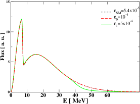
In the SM case, for the displayed energies, no transition can be seen for the flux in Fig.3.
For $\varepsilon=10^{-4}$, the transition cannot be seen since it is above $E_{\nu}\simeq 50$ MeV. Indeed, at this energy, though $<P(\nu_{e}\rightarrow\nu_{e})>_{\rm{exit}}$ is modified by the $\mu-\tau$ resonance, the difference between the initial $\nu_{e}$ and $\nu_{x}$ fluxes is too small to produce sizeable effects on the final $\nu_{e}$ flux on Earth (See Eq.(13)).
For $\varepsilon=5\times 10^{-4}$, a type B behaviour appears at $E_{\nu}\gtrsim 36$MeV whereas the type C behaviour is reached for $E_{\nu}\simeq 50$ MeV.
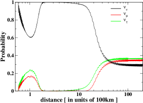
In the right part of Fig.(3), we show the oscillating probabilities for an energy below $E_{c}$ in the SM case. $E_{c}$ is known as the spectral split energy and here $E_{c}\simeq 8$ MeV. Looking at the electron neutrino survival probability, we see clearly the salient features of the $\nu-\nu$ interaction: the synchronization regime (for $r\lesssim 60$km), a bipolar transition until the spectral split climb-up occurs (for $r\simeq 100$km), which makes the probability goes back up to $\simeq 1$ (for $r\simeq 200$km). For this value of $N_{\mu\tau}$ and the energy considered, the $\mu\tau$ resonance position is well below the synchronization regime. Therefore, only type A behaviour occurs. The presence of $V_{\mu\tau}$ can only be seen through the fact that the bipolar transition occurs for both $\nu_{\mu}$ and $\nu_{\tau}$ neutrinos as consistent with Fig.(4) and the dashed arrow A. In conclusion, in this region of $N_{\mu\tau}$, the $\mu-\tau$ resonance happens before the bipolar region, hence the $\nu_{e}$s undergo a type A behaviour as defined above for $E_{\nu}\lesssim 36$MeV.

Figure 4: Level crossing scheme of neutrino conversion for the inverted hierarchy in a medium with a large $V_{\mu\tau}$ with $\theta_{23}$-mixing in the first octant and an neutrino energy $E_{\nu}<E_{c}$.

4.2 Case II

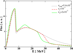
We can define this case for $\nu_{e}$s that undergo a type B transition for energies between $E_{\nu}\simeq E_{c}$ and $E_{\nu}\simeq 50$ MeV. Such behaviour corresponds to the interval $1.5\times 10^{6}$ g.cm${}^{-3}\lesssim N_{\mu\tau}\lesssim 2\times 10^{7}$g.cm^-3. For our density, the upper bound corresponds to $\varepsilon\simeq 7\times 10^{-3}$ while the lower bound is associated to $\varepsilon\simeq 5\times 10^{-4}$. We show in Fig.(5) two examples of such large $\varepsilon$ value: $\varepsilon=10^{-3}$ and $2\times 10^{-3}$. We also show, for comparison purpose, the $\nu_{e}$ flux for the SM value of $\varepsilon$. For $\varepsilon=10^{-3}$, the transition zone appears for $28$ MeV $\lesssim E_{\nu}\lesssim 33$ MeV.
For the case $\varepsilon=2\times 10^{-3}$, $P(\nu_{e}\rightarrow\nu_{e})$ leaves a type A behaviour for $E_{\nu}\gtrsim 10$ MeV and the type C behaviour is reached for $E_{\nu}\gtrsim 30$ MeV. In this case, we therefore have a larger transition zone, which is due to the fact that the resonance width is bigger. Indeed, this resonance width being proportional to $r_{\mu\tau}$, it varies like $(\varepsilon E\lambda_{r})^{\frac{1}{3}}$, and therefore gets larger when $\varepsilon$ goes from 10^-3 to 2 $\times 10^{-3}$. 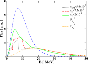This is why the flux moves away from the $\nu_{x}$ initial flux for the $E_{\nu}\sim 15$ MeV, i.e $<P(\nu_{e}\rightarrow\nu_{e})>_{\rm{exit}}$ is close but not equal to zero. For instance, at $E_{\nu}=15$ MeV, $<P(\nu_{e}\rightarrow\nu_{e})>_{\rm{exit}}$=0.15 which implies, recalling Eq.(13), $\Phi_{\nu_{e}}=0.15\times(F^{R}_{\nu_{e}}-F^{R}_{\nu_{\mu}})+F^{R}_{\nu_{\mu}}$. For $E_{\nu}\sim 20$ MeV, it seems, in a misleading way that the $<$ P$(\nu_{e}\rightarrow\nu_{e})$ $>_{\rm{exit}}$ has gone down to a zero value again. Actually, this is due to the fact that, for this energy, the initial fluxes of $\nu_{e}$ and of $\nu_{x}$ cross. Consequently, the $\nu_{e}$ flux on Earth is equal to the initial flux of $\nu_{x}$ for $E_{\nu}\sim 20$ MeV. Indeed, we can verify that the type B behaviour starts anew for $20$ MeV $<E_{\nu}<30$ MeV.

In the right part of Fig.(5), we show the oscillating probabilities for an energy below $E_{c}$. For this value of $N_{\mu\tau}$, the $\mu\tau$ resonance position is mainly below the bipolar transition. Nevertheless, it leads to a small disruption of the spectral split climb-up since the electron neutrino survival probability does not goes up back to a value of $\simeq 1$ but goes to $\simeq 0.93$ instead. $<P(\nu_{e}\rightarrow\nu_{e})>_{\rm{exit}}$ is slightly above the one yielded in case I. This explains the non perfect superimposition of the flux for energy below $E_{c}$. Note that the precise interplay between the $\mu\tau$ resonance and the neutrino-neutrino interaction in this case should be investigated more deeply.

  

Figure 5: Left figure: $\nu_{e}$ flux on Earth as a function of the energy for three different values of $\varepsilon$. Right figure: Oscillation probabilities as a function of the distance from the neutrinosphere with $\varepsilon=2\times 10^{-3}$ and $E_{\nu}=5.7$ MeV. We show the average as dashed lines and the envelopes of the fast-oscillating curves as solid lines.

4.3 Case III

We can define this case by the interval $2\times 10^{7}$g.cm${}^{-3}\lesssim N_{\mu\tau}\lesssim 6\times 10^{7}$g.cm^-3. For our density, the upper bound corresponds to $\varepsilon\simeq 2\times 10^{-2}$ while the lower bound is $\varepsilon\simeq 7\times 10^{-3}$. We show in Fig.(6) two examples for $\varepsilon=7.5\times 10^{-3}$ and $2\times 10^{-2}$ exhibiting two different cases. Note that in the case III, $\Delta r_{\mu\tau}$ is significantly greater than in the previous cases I and II because it varies as $\propto r_{\mu\tau}$.

In the case III, the $\mu-\tau$ resonance goes out of the synchronized region for $E\lesssim E_{c}$ where $E_{c}$ is the energy where the split occurs. Thus it will create a disruption of the spectral split phenomenon.
In the case $\varepsilon=7.5\times 10^{-3}$, we surprisingly see that a type A behaviour occurs for $E_{c}\lesssim E_{\nu}\lesssim$ 40 MeV. It turns out that the bipolar transition for theses energies is extremely disrupted. This may be due to a non-linear interference between the bipolar transition and the width of the $\mu-\tau$ resonance but this should deserve further investigation. For $E\gtrsim$ 40 MeV, we begin a transition phase.
In the case $\varepsilon=2\times 10^{-2}$, for $E_{\nu}\gtrsim E_{c}$, $r_{\mu\tau}+\frac{\Delta r_{\mu\tau}}{2}>r_{bip}$, this corresponds to the beginning of the transition phase which lasts till $r_{\mu\tau}-\frac{\Delta r_{\mu\tau}}{2}>r_{bip}$. It is important to note that the more the energy increases the larger the resonance width is, so the phase transition begins for $E_{\nu}\lesssim E_{c}$. Note that the spectral split signature is vanishing for this value of $\varepsilon$.

  

Figure 6: Left figure: $\nu_{e}$ flux on Earth as a function of the energy for three different values of $\varepsilon$. We also show here the initial $\nu_{e}$ and $\nu_{x}$ flux emitted at the neutrinosphere. Right figure: Oscillation probabilities as a function of the distance from the neutrinosphere with $\varepsilon=7.5\times 10^{-3}$ and $E_{\nu}=5.7$ MeV. We show the average as dashed lines and the envelopes of the fast-oscillating curves as solid lines.

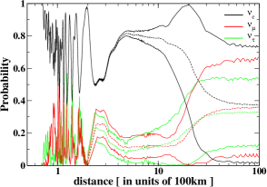
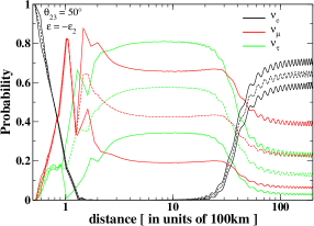
The disruption of the spectral split phenomenon is explicitly shown in the right part of Fig.(6). The bipolar transition shows huge oscillations due to a powerful interplay with the $\mu\tau$ resonance, while the spectral split climb-up makes the electron survival probability go up only to a value of $\simeq 0.8$ (see right part of Fig(6)) contrary to the SM case where it goes back up to $\simeq 1$. Eventually, this leads to a higher value of $<P(\nu_{e}\rightarrow\nu_{e})>_{\rm{exit}}$ which was seen on the left part of Fig.(6). This phenomenon is represented in Fig.(4) by the wiggled arrow B.

Finally, note that in this section, since we studied the influence of an increasing value of $\varepsilon$, we have displayed in the three cases the oscillating probabilities with $E_{\nu}<E_{c}$. Indeed, as $\varepsilon$ increases, the resonance occurs for lower and lower energies since the density remains in the three cases constant. This can be seen in Eq.(17). It is therefore interesting to look at the evolution of the probabilities at the energy around which the $\mu-\tau$ resonance occurs. The evolution probabilities for $E_{\nu}>E_{c}$ can be seen in Figs. (1).

5 The degeneracy of $\varepsilon$ with respect to other parameters

As seen in Sec. 3, the typical behaviour A, B or C are the consequence of a certain position of the $\mu-\tau$ resonance in comparison with the bipolar transition. In the following subsections, we study in particular one parameter that influence either the resonance or the $\nu-\nu$ interaction, the other being fixed to their reference value as defined in Sec. 2.

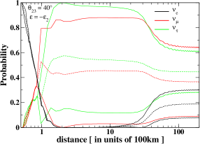
5.1 Effects of $\theta_{23}$ and of the sign of $\varepsilon$

Changing the value of $\theta_{23}$ in such way that it changes of octant, will automatically prevent a $\mu-\tau$ resonance as discussed in [30, 45]. Using the two flavour MSW condition,

$$\frac{\Delta m^{2}_{atm}}{2E_{\nu}}\cos 2\theta_{23}=V_{\mu\tau}=\varepsilon\sqrt{2}G_{F}Y_{e}\rho_{B},$$ (22)

one can see that changing the sign of $\varepsilon$ could be immediately interpreted as perfectly equivalent to changing of octant. However, in the case of a negative $\varepsilon=-|\varepsilon|$, looking at the matter interaction Hamiltonian, we have:

$$H_{m}=diag(V_{e},0,-|V_{\mu\tau}|)=diag(V_{e}+|V_{\mu\tau}|,|V_{\mu\tau}|,0).$$ (23)

In this case, the term $|V_{\mu\tau}|$ becomes a matter potential for $\nu_{\mu}$ which can be seen like an effective presence of muon in the supernova whereas the electron matter potential appears slightly modified of the order of $\varepsilon$, i.e $2\%$ at most.

This explains why, looking at the left figure panel in Fig.(7), the top and lower part show opposite behaviours for $\nu_{\mu}$ and $\nu_{\tau}$ in the first 100km; The same thing happens for the right figure panel. Even when the MSW condition is not fulfilled, a matter effect is still present as can be seen in [30]. This is called the matter suppression effect and a transition, though partial is happening.

   

   

Figure 7: Oscillation probabilities as a function of the distance from the neutrinosphere. We show the average as dashed lines and the envelopes of the fast-oscillating curves as solid lines. The figures correspond to the value of the couple of parameters ($\varepsilon=\pm\varepsilon_{2}$, $\theta_{23}=40^{\circ}$ or $50^{\circ}$). $\varepsilon_{2}$ is still equal to $2\times 10^{-3}$. In these figures, the neutrino energy is 30 MeV.

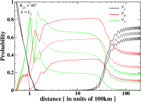
In Fig.(8), we observe that the energy spectra of the electron neutrino flux on Earth, is the same for the parameter couples ($\varepsilon>0$, $\theta_{23}=40^{\circ}$) and ($\varepsilon<0$, $\theta_{23}=50^{\circ}$) whereas a identical shift for the transition around 30 MeV is observed in the cases ($\varepsilon<0$, $\theta_{23}=40^{\circ}$) and ($\varepsilon>0$, $\theta_{23}=50^{\circ}$). The fact that a similar behaviour between the cases ($\varepsilon>0$, $\theta_{23}=40^{\circ}$) and ($\varepsilon<0$, $\theta_{23}=50^{\circ}$) is observed is due to the fulfillment of the MSW condition (Eq.(22)) in the two cases. The only differences can be seen on the evolution with the distance of the $\nu_{\mu}$ and $\nu_{\tau}$ oscillation probabilities, as said above because in the first/second case, the neutrinos see respectively an effective presence of $\tau$/$\mu$ leptons. In the opposite cases, no MSW resonance can happen but a matter suppression effect occurs. To explain this shift in energy, one can think the matter suppression as a transition between $\nu_{\mu}$ and $\nu_{\tau}$ neutrinos but less effective as the MSW resonance. Since in all cases, all the parameters except the sign of $\varepsilon$ and the octant of $\theta_{23}$, are identical, to maximize the effect of this matter suppression, one needs to move it away from the collective effects region, this can be done by increasing the neutrino energy. Note that the matter suppression can interfere with the collective effects as represented as a wiggled arrow in Fig.(9).

Figure 8: $\nu_{e}$ flux on Earth as a function of the energy for different values of the parameter couple ( $\varepsilon$, $\theta_{23}$). $\varepsilon_{2}$ is still equal to $2\times 10^{-3}$.

Figure 9: Level crossing scheme of neutrino conversion for the inverted hierarchy in a medium with a large $V_{\mu\tau}$ with $\theta_{23}$-mixing in the second octant.

5.2 Effects of the luminosity

Effects of luminosity should not be neglected. As the cooling phase passes, the neutrino fluxes emitted at their respective neutrinosphere, decrease in intensity. Such diminution can be approximated by a decreasing exponential as seen in Eq.(12). Consequently, the strength of the $\nu-\nu$ interaction shrinks, implying a slow diminution of the collective effect predominating zone:

$$r_{bip}\sim\mu_{0}^{\frac{1}{4}}\sim\exp\left(\frac{-t}{4\tau}\right)$$ (24)

As the bipolar radius decreases, $r_{\mu\tau}$ being fixed, the electron neutrino probability behaviour tends to be like the type C behaviour. This can be seen in Fig.(10) where the fluxes have been normalized to the reference value in order to appreciate only the $\mu-\tau$ / $\nu-\nu$ interplay effects. Knowing that $r_{\mu\tau}\sim(\lambda_{r}\varepsilon)^{\frac{1}{3}}$, multiplying the luminosity by a factor $\alpha$ would in principle be equivalent to multiply either $\lambda_{r}$ or $\varepsilon$ by a factor $\alpha^{\frac{-3}{4}}$ since

$$\frac{r_{\mu\tau}}{r_{bip}}\sim(\lambda_{r}\varepsilon)^{\frac{1}{3}}\mu_{0}^{\frac{-1}{4}}$$ (25)

Therefore, increasing the luminosity or shifting inwards the position of the $\mu-\tau$ resonance is rather equivalent until the neutrino density is too weak to maintain collective effects.

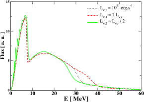
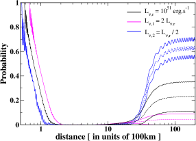
Looking at the left part of Fig.(10), one sees the energy spectra of $\nu_{e}$ varying as predicted above. When $L_{\nu}=2\times 10^{51}$erg.s^-1 the $\nu_{e}$ present a similar shape with the reference case, except that the transition zone starts for $E_{\nu}\simeq 35$ MeV. Indeed, a higher luminosity is equivalent to a $\mu-\tau$ resonance position deeper inside the supernova. Therefore, neutrinos need a higher energy value to begin to see the type B behaviour. Symmetrically, a lower value of the initial neutrino flux will make the type B behaviour appears for lower energies, i.e $E_{\nu}\simeq 23$ MeV in this case. Note that because of a low value of the neutrino flux, the collective effects start to weaken which leads to some oscillations in the flux for energies $E_{\nu}\lesssim E_{c}$. Equivalently, one can look at the right part of Fig.(10) where we show the electron neutrino survival probability for the three different values of the luminosity: $L_{\nu,r}$, $L_{\nu,1}$ and $L_{\nu,2}$. The value of $<P(\nu_{e}\rightarrow\nu_{e})>_{\rm{exit}}$ is anew highly dependent of the relative position of $r_{\mu\tau}$ w.r.t $r_{bip}$. This figure shows explicitly the increase of $r_{bip}$ with the luminosity.

  

Figure 10: Left figure: luminosity-normalized $\nu_{e}$ flux on Earth as a function of the energy for three different luminosities. Right figure: Electron neutrino survival probabilities as a function of the distance from the neutrinosphere for three different luminosities with $E_{\nu}=30$ MeV. We show the average as dashed lines and the envelopes of the fast-oscillating curves as solid lines.

5.3 Effects of the density

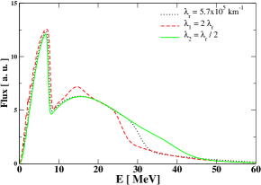
Depending on the mass of the progenitor star, the explosion releases a variable energy which, under the form of a shock-wave, can lead to important variation on the matter density, whose precise profile remains partially unknown. In our analytical profile, it means that the value of $\lambda_{r}$ will decrease with time. The effect of the density variation through the parameter $\lambda_{r}$ is crystal clear. Using Eq.(17), one can see that the position of the $\mu-\tau$ resonance varies like $\lambda_{r}^{\frac{1}{3}}$. Therefore, changing the density or the value of the radiative correction term $\varepsilon$ is almost perfectly equivalent as long as the density does not reach very high value such as in the accretion phase. This can be seen in the left part of Fig.(11) where the density is $\lambda_{1}=2\lambda_{r}$ and $\lambda_{2}=\lambda_{r}/2$ are respectively equivalent to the reference case but with $\varepsilon_{1}=2\times 10^{-3}$ and $\varepsilon_{2}=5\times 10^{-4}$. The incertitude concerning the density profile plays an important role as $N_{\mu\tau}$ gives rise to three well distinct behaviours corresponding to the cases I, II and III. Equivalently, one can look at the right part of Fig.(11), where we show the electron neutrino survival probability for the three different values of the density: $\lambda_{r}$, $\lambda_{1}$ and $\lambda_{2}$; We can notice that $r_{bip}$ is the same for the three curves, which is consistent with the fact that the luminosity has not been modified. The bipolar transition is a bit disrupted in the case where the matter is more dense. This is due to the fact that the $V_{\mu\tau}$ term is larger, which implies a more powerful interplay with the $\mu-\tau$ resonance. Moreover, we see a light shift of the L-resonance position towards the outside of the supernova with an increasing value of the density parameter $\lambda$.

  

Figure 11: Left figure: $\nu_{e}$ flux on Earth as a function of the energy for three different densities. Right figure: Electron neutrino survival probabilities as a function of the distance from the neutrinosphere for three different densities with $E_{\nu}=30$ MeV. We show the average as dashed lines and the envelopes of the fast-oscillating curves as solid lines.

6 Detection of the signal on Earth

Since the explosion of SN1987A in the Large Magelanic Cloud, it has been proved that neutrinos from supernova can be detected on Earth. Such astrophysical event can yield a tremendous amount of information through the neutrino fluxes received on Earth. With the currently running neutrino observatories, a high-statistics signal for a galactic SN explosion is expected in the electron anti-neutrino channel. For instance, Super-Kamiokande could detect through the reaction $\bar{\nu}_{e}+p\rightarrow n+e^{+}$ about $\sim 10^{4}$ events. Nevertheless, larger detectors could yield an even better statistics and therefore could be sensitive to more discreet features of the explosion. Also, they logically could detect a more distant explosion with the same current number of event statistics.

Three main types of multi-purpose detectors are proposed to enhance the quality of information about the neutrino properties and the explosion mechanism that we will receive from the supernova neutrino fluxes. The proposed future neutrino observatories offered complementary detection techniques: a megaton water Cherenkov detector such as MEMPHYS or Hyper-Kamiokande, a liquid scintillator like LENA or a liquid argon Time Projection Chamber (TPC) like GLACIER. See e.g. [46] for a detailed review on those large-scale future detectors. The interest of such detectors, for a supernova neutrino signal, has been showed e.g. in [40] for the water-Cherenkov type or in [37] for a liquid Argon type. We focus on a detector of the latter kind since it has the possibility to detect electron neutrino by charged-current, through the reaction

$$\nu_{e}+^{40}{\rm Ar}\rightarrow^{40}{\rm K^{*}}+e^{-}$$ (26)

therefore yielding a very clear signal complementary of the inverse $\beta$ of the water Cherenkov detectors.

To calculate the number of events received in such liquid Argon detector (Icarus-like), we use the cross section given in [37] for the charged-current reaction (26). For the detection of the $\mu-\tau$ resonance effect in a liquid Argon type experiment, we calculate the usual differential number of neutrinos detected at a distance D from the supernova:

$$\frac{d^{2}N_{events}}{dE_{\nu}dt}=\frac{N_{targets}}{4\pi D^{2}}\frac{d^{2}N_{\nu}}{dE_{\nu}dt}\sigma(E_{\nu})$$ (27)

where $N_{targets}$ is the number of targets in the detector, D is the distance from the supernova, $E_{\nu}$ is the neutrino energy, t is the detector time, $d^{2}N_{\nu}/dE_{\nu}dt$ the differential flux of neutrinos arriving on Earth, for a given detector time and a given neutrino energy, and $\sigma(E_{\nu})$ is the cross section of the reaction process considered. For a galactic explosion, we suppose that the supernova explosion will happen at the distance $D=10$kpc. Our calculations do not include Earth matter effects and the Poisson error due to the finite number of detected events.

For the signal really obtained in the detector, note that the energy resolution reached in the detector is good enough to appreciate precisely the $\mu-\tau$ resonance effect. Indeed, the energy of the neutrino will not be directly obtained. It will be accessible via the electron energy of the reaction of Eq.(26).

In a realistic supernova environment, after the post-bounce, both the density profile and the luminosity are decreasing. As seen in the previous section, this affects the interplay between the $\mu-\tau$ resonance and the $\nu-\nu$ interaction. If the density decreases, the $\mu-\tau$ resonance tends to get closer from the nascent iron core with $r_{\mu\tau}\sim\lambda_{r}^{\frac{1}{3}}$. When the luminosity decreases, the bipolar region shrinks as $r_{bip}\sim\L_{\nu}^{\frac{1}{4}}$. Those two phenomena are therefore opposite and tend to provoke a status quo concerning the type of behaviour of the electron neutrino flux. The way the $\nu_{e}$ flux energy distribution is modified with time depends on the relative variation speed of the parameters $\lambda_{r}$ and $\L_{\nu}$.

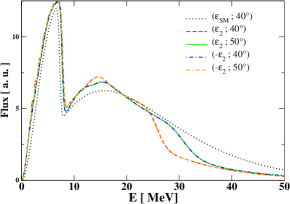
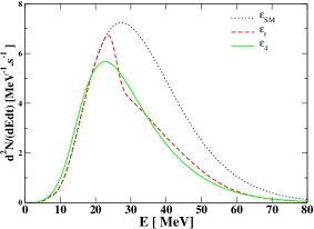
Of course, the absolute value of the flux will undergo a global exponential decrease with time. In the literature tackling the question of dynamical density profile induced by shock-waves, the difference of density during a time variation of about 5s, tends to be of a factor $\sim 2$, for the part of the density which can be well approximated by a power-law. See e.g. [48] for the density profile as a function of time. In Figs.(12) and (13), we show the differential number of events received in a 70kton liquid argon type detector and the associated flux for a post-bounce time of 3 and 8 s. We study three distinct values for the radiative correction term $\varepsilon$: the SM value $\varepsilon_{SM}=5.4\times 10^{-5}$ whose $N_{\mu\tau}$ will stay in region I for these two times, an intermediate value $\varepsilon_{r}=10^{-3}$ which corresponds for the $\nu_{e}$ flux to a case II behaviour until 8s, and the typical maximum value obtained in the SUSY framework, i.e $\varepsilon_{4}=2\times 10^{-2}$ which corresponds for the $\nu_{e}$ flux to case III behaviour during most of the cooling phase.

   

Figure 12: In this case, the time after post-bounce is supposed to be t=3s, the initial luminosity taken is $L_{\nu}(t=3s)=4.24\times$ 10⁵¹ erg.s^-1, the density parameter is $\lambda_{r}$ = 1.14 $\times$ 10⁶ and $\theta_{23}$ = 40^∘. Left figure: differential number of events on Earth in a Liquid Argon detector of 70 kton size as a function of the energy for three different $\varepsilon$. Right figure: corresponding $\nu_{e}$ flux on Earth as a function of the energy for three different $\varepsilon$.

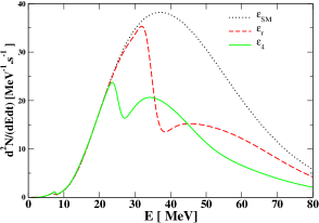
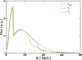
For $t=3s$, the neutrino fluxes with $\varepsilon_{r}$ or $\varepsilon_{4}$ entering the detector show important differences with the SM case. While for $\varepsilon_{r}$ the difference with $\varepsilon_{SM}$ appears for an energy of $\simeq 32$MeV as a sizeable decrease of flux, the difference for $\varepsilon_{4}$ appears at a lower energy $\simeq 22$MeV. Looking at the differential number of events, we see that the usual spectral split feature becomes almost invisible except in the case of $\varepsilon_{4}$ where a very small bump remains. On the contrary the effects of the $\mu-\tau$ resonance at higher energies are much more visible. In the case of $\varepsilon_{r}$, a new spectral split feature appears. A type B behaviour starts at $\simeq 32$ MeV and leads to a type C behaviour from $\simeq 38$ MeV. For $\varepsilon_{4}$, the flux undergoes a diminution from $\simeq 22$MeV but this split feature is not as salient as the previous one. Nevertheless, we see that in the $\varepsilon_{4}$ case, the number of events is globally smaller than the $\varepsilon_{r}$ case. With respect to the SM case, the difference in the number of events corresponds in average to a factor $\sim$2 from $\simeq 22$ MeV.

   

Figure 13: In this case, the time after post-bounce is supposed to be t=8s, initial luminosity taken is $L_{\nu}$(t=8s) = 10⁵¹ erg.s^-1, the density parameter is $\lambda_{r}$ = 5.7 $\times$ 10⁵ and $\theta_{23}$ = 40^∘. Left figure: differential number of events on Earth in a Liquid Argon detector of 70 kton size as a function of the energy for three different $\varepsilon$. Right figure: corresponding $\nu_{e}$ flux on Earth as a function of the energy for three different $\varepsilon$.

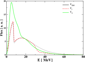
For $t=8s$, the neutrino fluxes with $\varepsilon_{r}$ or $\varepsilon_{4}$ display a modification w.r.t the SM case similarly to time $t=3$s. Concerning the flux with $\varepsilon_{r}$, it leaves the type A behaviour for a lower energy equals to $\simeq 28$ MeV. this can be understood recalling Eq.(25). Indeed, since $\lambda_{r}$ has been multiplied by a factor 0.5 and the luminosity has decreased by a factor $\simeq 4$, the relative position of $r_{\mu\tau}$ over $r_{bip}$ has increased by a factor $\simeq 4^{\frac{1}{4}}2^{-\frac{1}{3}}>1$. Consequently, a lower energy is required for the type B behaviour to start. Concerning the flux with $\varepsilon_{4}$, the relative difference w.r.t. the flux in the SM case is more important at low energies. Nevertheless, the luminosity being exponentially decreasing with time and the low value of the cross-section at low energies will prevent to see the effects of $\varepsilon_{4}$ on the number of events for those energies. Finally, we can see on the number of events figure, that the $\varepsilon_{r}$ curve presents globally a more pronounced difference w.r.t to the SM case than the $\varepsilon_{4}$ curve.

   

Figure 14: In this case, the time after post-bounce is supposed to be t=8s, initial luminosity taken is $L_{\nu}$(t=8s) = 10⁵¹ erg.s^-1, the density parameter is $\lambda_{r}$ = 5.7 $\times$ 10⁵ and $\theta_{23}$ = 40^∘. In these figures the hierarchy in temperature is $\langle E_{\nu_{e}}\rangle=12$ MeV, $\langle E_{\bar{\nu}_{e}}\rangle=15$ MeV, $\langle E_{\nu_{x}}\rangle=18$ MeV. Left figure: differential number of events on Earth in a Liquid Argon detector of 70 kton size as a function of the energy for three different $\varepsilon$. Right figure: corresponding $\nu_{e}$ flux on Earth as a function of the energy for three different $\varepsilon$.

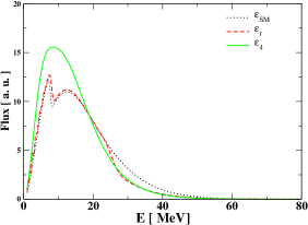
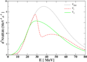
In Fig.(14), we take other values for the energy hierarchy in agreement with the numerical simulations performed in [49]: i.e. $\langle E_{\nu_{e}}\rangle=12$ MeV, $\langle E_{\bar{\nu}_{e}}\rangle=15$ MeV, $\langle E_{\nu_{x}}\rangle=18$ MeV respectively. Concerning the flux with $\varepsilon_{r}$, the difference w.r.t the SM case appears from $\simeq 23$ MeV. For $\varepsilon_{4}$, the spectral split feature has vanished and the flux presents a much higher value w.r.t the SM case around 10 MeV. Concerning the number of events, both $\varepsilon_{r}$ and $\varepsilon_{4}$ curves move away from the SM one from around 20 MeV. We therefore conclude that even with this hierarchy of temperatures, sizeable effects are present on the differential number of events received in a Liquid Argon detector.

Though we did not look at the time evolution $\nu_{e}$ flux for given energies during the whole cooling phase, it seems that the global pattern of the fluxes will not be much modified with time, contrary to what may happen for the electron anti-neutrino flux [34]. In this case, to distinguish w.r.t. the SM case would require the identification of a particular energy distribution of the flux.

Considering the $\nu_{e}$ flux, for the $\varepsilon_{r}$ case, the spectral split feature seems peculiar enough to be recognized: at 40 MeV, the ratio between the SM flux and the $\varepsilon_{r}$ flux is more or less constant. One could also look at the time evolution of the flux for an energy of 30 MeV and 40 MeV. In the SM case, the flux at 40 MeV will be systematically higher than the one at 30 MeV. In the case of a large $\varepsilon$, the flux at 40 MeV will be systematically lower. For the $\varepsilon_{4}$ case, the low energy bump may be visible for early time because of an important global luminosity. Therefore, the presence of a spectral split at high energy in the differential number of events may be a signature of a large radiative correction term and therefore a beyond standard physics.

Using the signal in the electron anti-neutrino channel with a Cherenkov detector, one would be able to obtain precise information on the density profile as a function of time. In addition, with enough precision on the neutrino parameters, like the octant of $\theta_{23}$, as well as Supernova parameters partly given by the other channels (electron anti-neutrino via inverse $\beta$ reaction, all flavour flux via neutral current), this could ideally lead to new constraints for the SUSY parameters via the analytical calculation of the radiative correction as in [33, 24]. Equivalently, the absence of such characteristic imprints would also lead to constraints if no other effects like turbulence modify the $\nu_{e}$ flux existing inside the supernova as will be discussed in the next section.

Finally, note that the impact of the interplay between $V_{\mu\tau}$ and the collective effects has been observed on the Diffuse Supernova Neutrino Background (DSNB) [35]. Such interplay tends to provoke important effects even in the Standard Model thanks to the redshift.

7 Discussions

In this section we discuss on how much these results can be seen as realistic.

We have performed a calculation of the neutrino propagation in a core-collapse supernova including the neutrino-neutrino interaction and a large mu-tau index of refraction coming from SUSY radiative corrections. Such combination in certain conditions of matter density, energy, luminosity and oscillation parameters implies a resonance, associated to the loop correction potential. This occurs in the same region as the bipolar resonance. Consequently, the $\nu_{\mu}$ and $\nu_{\tau}$ oscillation probabilities are modified and the low-resonance becomes much more adiabatic leading to an important inversion of fluxes, visible on the electron neutrino flux on Earth as a function of energy. Such characteristic imprints of a large $V_{\mu\tau}$, i.e of a BSM physics, would be also sizeable on the number of events in a Liquid Argon detector type.

In a supernova environment, such interplay has been first studied for a given energy in [30]. In order to obtain a $\mu-\tau$ resonance with a radiative correction term in the SM framework, the authors considered a very high density profile. This way, such resonance happens well outside the bipolar transition zone and a clear, easily understandable, behaviour is exhibited. Unfortunately, it has been shown in [21], for the multi-angle and, therefore, general case, that such high density prevents collective effect from taking place. Consequently, we have to check if the density we use is low enough for the multiangle matter effect to be neglected. In [45], they found that the condition:

$$Y_{e}(r_{syn})\lambda_{r}\frac{R}{r_{syn}}<\mu_{0}$$ (28)

must be fulfilled. Using Eq.(11) of [44], we find in our case, $\mu_{0}\simeq 2.6\times 10^{5}$ km^-1. Therefore, having $Y_{e}=0.5$ and assuming $r_{syn}\simeq 100$ km the condition becomes : $\lambda_{r}<5.2\times 10^{6}$ km^-1. Since $\lambda_{r}=5.7\times 10^{5}$ km^-1, we can indeed safely neglect the matter effects.

The advantage of having a large $V_{\mu\tau}$ potential due to a large SUSY radiative correction is significant for multiple reason. In this case, a very high density is not required for the $\mu-\tau$ resonance to be outside the zone where collective effects predominate. Therefore, we naturally avoid the problem of the high density effect cited above.

Concerning our density profile, we use an analytical power law which does not take into account shock-waves effects. Nevertheless we believe such dynamical effects are not determinant in our case. Indeed, we checked [50] that the shock-wave effects such as depicted in [34] do not affect the $\nu_{e}$ flux. In inverted hierarchy, $\nu_{e}$s do not encounter the H-resonance, and therefore do not undergo the effect of adiabaticity breaking and/or multiple resonance which tends to smear out the neutrino flux distribution. Moreover, looking at the $\nu_{e}$ flux during the cooling phase not too early, allows the shock wave to affect the density profile well after 1000 km, i.e well after that the $\mu-\tau$ resonance and the $\nu-\nu$ interaction occur. Similarly, the L resonance is not supposed to be significantly affected by the shock-wave effects [41].

Concerning the collective effects, even if the matter density is not so high, multi-angle should be prevented of triggering decoherence because of the asymmetry between the $\nu_{e}$ and $\bar{\nu}_{e}$ flux cause by deleptonization [44]. Consequently, single-angle behaviour may well be typical for realistic SN conditions as long as this flux asymmetry remains.

Note that we have checked that the influence of $\delta$ is negligible in this particular case where we focus on the electron neutrino signal in the inverted hierarchy. Moreover, we took equal luminosities for $\nu_{\mu}$ and $\nu_{\tau}$ flux [27]. As long as it is non zero, the influence of $\theta_{13}$ on the $\nu_{e}$ flux in inverted hierarchy is very small, possibly below the experimental uncertainties.

In our paper, we also made the assumption of a constant electron fraction. This approximation is justified when we restrict ourselves to a maximum value of $\simeq 2\times 10^{-2}$ for radiative term $\varepsilon$. In this case, no non-standard interaction (NSI) resonance will occur as shown in [45]. 

Similar interplay should be in principle present in the anti-neutrino channel but as pointed out in [34], the presence of shock-waves effects tend to render the H-resonance non adiabatic and eventually create a multiple resonance effect which can smear out the electron anti-neutrino signal. The addition of such important radiative correction matter potential should disturb the signal but full numerical calculation as first performed in should be done to witness the impact on the electron anti-neutrino flux.

Concerning the normal hierarchy, the effects of the $\mu-\tau$ resonance tend to be much smaller as no bipolar transition occurs. Nevertheless, the case where spectral splits take place in this hierarchy [51, 52] should be investigated in the presence of a large $\varepsilon$.

Finally, we discuss the most important effect that could prevent the salient modification of the $\nu_{e}$ flux induced by the $\mu-\tau$ resonance and $\nu-\nu$ interplay. A realistic density profile should present possible stochastic matter fluctuations due to hydrodynamical instabilities created in the wake of a shock front. This has been studied in several works [53, 54] but the precise size of such fluctuations remains an important open issue. In principle, the $\mu-\tau$ resonance should not be affected. The question whether the L-resonance will be affected or not, depends on the fluctuation scale i.e if the damping effects are significant on the flavour transition pattern. Associated with this issue, taking into account a non-spherical symmetry for the neutrino emission [55] as well with matter density profile [41], may be relevant, for example, in the presence of hydrodynamic turbulence in the background of ordinary matter. The framework considered in this paper, defined in Sec. 2, allows us to think that our results should contain the main features of a realistic signal.

8 Conclusion

In this paper, we worked in the SUSY framework. If new phenomena compatible with this framework are discovered on the supernova neutrino fluxes, one of the major challenges will be to find out the underlying model and to measure its parameters as precisely as possible. This can be done for example by using codes in which we consider the phenomenological constraints [56]. It will be necessary to investigate the precision with which SUSY model parameters [33] can be derived from these measurements. Finally, if Supersymmetry is realised in Nature, it should be possible to constrain the SUSY parameters thanks to the discovery of sparticles at TeV colliders. For a galactic explosion, using a fully detailed numerical simulation, supernova neutrino fluxes could ideally lead to constraints on the SUSY parameters in the inverted hierarchy case. In the future, the results presented in this paper should be applied to a larger variety of models and confronted to some other data from the Large Hadron Collider (LHC) and the International Linear Collider (ILC). Finally, let us say that the $\mu-\tau$ resonance effect on the energy distribution of the electron neutrino flux could impact on the number of events for relic supernova neutrinos as in [35]. In this case, it could give an even lower total red-shift-integrated number of events than in the SM case which can be consistent with observations. Moreover, a large $\varepsilon$ could also impact the heavy elements nucleosynthesis in supernova, and more precisely on the electron fraction through the r-process. Supernovae can definitively be seen more than ever, as an open window towards beyond Standard Model physics.

References

- [1] L. Wolfenstein, Phys. Rev. D 17, 2369 (1978);20, 2634 (1979)
- [2] S. P. Mikheev and A. Y. Smirnov, Nuovo Cim. C 9, 17 (1986).
- [3] J. T. Pantaleone, Phys. Lett. B 287, 128 (1992).
- [4] G. Sigl and G. Raffelt, Nucl. Phys. B 406, 423 (1993).
- [5] S. Samuel, Phys. Rev. D 48, 1462 (1993).
- [6] Y. Z. Qian and G. M. Fuller, Phys. Rev. D 51, 1479 (1995) [arXiv:astro-ph/9406073].
- [7] G. Sigl, Phys. Rev. D 51, 4035 (1995) [arXiv:astro-ph/9410094].
- [8] S. Pastor, G. G. Raffelt and D. V. Semikoz, Phys. Rev. D 65, 053011 (2002) [arXiv:hep-ph/0109035].
- [9] S. Pastor and G. Raffelt, Phys. Rev. Lett. 89, 191101 (2002) [arXiv:astro-ph/0207281].
- [10] A. B. Balantekin and H. Yuksel, New J. Phys. 7, 51 (2005) [arXiv:astro-ph/0411159].
- [11] H. Duan, G. M. Fuller and Y. Z. Qian, Phys. Rev. D 74, 123004 (2006) [arXiv:astro-ph/0511275].
- [12] H. Duan, G. M. Fuller, J. Carlson and Y. Z. Qian, Phys. Rev. D 74, 105014 (2006) [arXiv:astro-ph/0606616].
- [13] S. Hannestad, G. G. Raffelt, G. Sigl and Y. Y. Y. Wong, Phys. Rev. D 74, 105010 (2006) [Erratum-ibid. D 76, 029901 (2007)] [arXiv:astro-ph/0608695].
- [14] A. B. Balantekin and Y. Pehlivan, J. Phys. G 34 (2007) 47 [arXiv:astro-ph/0607527].
- [15] H. Duan, G. M. Fuller, J. Carlson and Y. Z. Qian, Phys. Rev. Lett. 97, 241101 (2006) [arXiv:astro-ph/0608050].
- [16] G. L. Fogli, E. Lisi, A. Marrone and A. Mirizzi, JCAP 0712, 010 (2007) [arXiv:0707.1998 [hep-ph]].
- [17] G. G. Raffelt and A. Y. Smirnov, Phys. Rev. D 76, 081301 (2007) [Erratum-ibid. D 77, 029903 (2008)] [arXiv:0705.1830 [hep-ph]].
- [18] G. G. Raffelt and A. Y. Smirnov, Phys. Rev. D 76, 125008 (2007) [arXiv:0709.4641 [hep-ph]].
- [19] H. Duan, G. M. Fuller, J. Carlson and Y. Z. Qian, Phys. Rev. Lett. 100, 021101 (2008) [arXiv:0710.1271 [astro-ph]].
- [20] B. Dasgupta and A. Dighe, Phys. Rev. D 77, 113002 (2008) [arXiv:0712.3798 [hep-ph]].
- [21] A. Esteban-Pretel, A. Mirizzi, S. Pastor, R. Tomas, G. G. Raffelt, P. D. Serpico and G. Sigl, Phys. Rev. D 78 (2008) 085012 [arXiv:0807.0659 [astro-ph]].
- [22] H. Duan and J. P. Kneller, J. Phys. G 36 (2009) 113201 [arXiv:0904.0974 [astro-ph.HE]].
- [23] F. J. Botella, C. S. Lim, and W. J. Marciano, Phys. Rev. D 35 (1987) 896.
- [24] E. Roulet, Phys. Lett. B 356 (1995) 264 [arXiv:hep-ph/9506221v1].
- [25] E. K. Akhmedov, C. Lunardini and A. Y. Smirnov, Nucl. Phys. B 643 (2002) 339 [arXiv:hep-ph/0204091].
- [26] H. Minakata and S. Watanabe, Phys. Lett. B 468 (1999) 256 [arXiv:hep-ph/9906530].
- [27] A. B. Balantekin, J. Gava and C. Volpe, Phys. Lett. B 662, 396 (2008) [arXiv:0710.3112 [astro-ph]].
- [28] J. P. Kneller and G. C. McLaughlin, Phys. Rev. D 80 (2009) 053002 [arXiv:0904.3823 [hep-ph]].
- [29] Jerome Gava, and Cristina Volpe, Phys. Rev. D 78, 083007 (2008) arXiv:0807.3418 [astro-ph].
- [30] A. Esteban-Pretel, S. Pastor, R. Tomas, G. G. Raffelt and G. Sigl, Phys. Rev. D 77, 065024 (2008) [arXiv:0712.1137 [astro-ph]].
- [31] H. Duan, G. M. Fuller and Y. Z. Qian, Phys. Rev. D 77, 085016 (2008) [arXiv:0801.1363 [hep-ph]].
- [32] J. Wess and J. Bagger, Supersymmetry and Supergravity, second ed., Princeton University Press, Princeton, 1992.
- [33] J. Gava and C.-C. Jean-Louis, Phys. Rev. D 81, 013003 (2010) arXiv:0907.3947 [hep-ph].
- [34] J. Gava, J. Kneller, C. Volpe and G. C. McLaughlin, Phys. Rev. Lett. 103 (2009) 071101 [arXiv:0902.0317 [hep-ph]].
- [35] S. Galais, J. Kneller, C. Volpe and J. Gava, Phys. Rev. D 81 (2010) 053002 [arXiv:0906.5294 [hep-ph]].
- [36] C. Amsler et al. [Particle Data Group], Phys. Lett. B 667 (2008) 1.
- [37] I. Gil Botella and A. Rubbia, JCAP 0310 (2003) 009 [arXiv:hep-ph/0307244].
- [38] A. S. Dighe and A. Y. Smirnov, Phys. Rev. D 62 (2000) 033007 [arXiv:hep-ph/9907423].
- [39] R. Tomas, M. Kachelriess, G. Raffelt, A. Dighe, H. T. Janka and L. Scheck, JCAP 0409 (2004) 015 [arXiv:astro-ph/0407132].
- [40] G. L. Fogli, E. Lisi, A. Mirizzi and D. Montanino, JCAP 0504 (2005) 002 [arXiv:hep-ph/0412046].
- [41] J. P. Kneller, G. C. McLaughlin and J. Brockman, Phys. Rev. D 77 (2008) 045023 [arXiv:0705.3835 [astro-ph]].
- [42] A. Mirizzi, S. Pozzorini, G. G. Raffelt and P. D. Serpico, JHEP 0910 (2009) 020 [arXiv:0907.3674 [hep-ph]].
- [43] M. Blennow, A. Mirizzi and P. D. Serpico, Phys. Rev. D 78 (2008) 113004 [arXiv:0810.2297 [hep-ph]].
- [44] A. Esteban-Pretel, S. Pastor, R. Tomas, G. G. Raffelt and G. Sigl, Phys. Rev. D 76, 125018 (2007) [arXiv:0706.2498 [astro-ph]].
- [45] A. Esteban-Pretel, R. Tomas and J. W. F. Valle, Phys. Rev. D 81 (2010) 063003 [arXiv:0909.2196 [hep-ph]].
- [46] D. Autiero et al., JCAP 0711 (2007) 011 [arXiv:0705.0116 [hep-ph]].
- [47] B. Dasgupta, A. Dighe and A. Mirizzi, Phys. Rev. Lett. 101 (2008) 171801 [arXiv:0802.1481 [hep-ph]].
- [48] C. Lunardini and A. Y. Smirnov, JCAP 0306 (2003) 009 [arXiv:hep-ph/0302033].
- [49] M. T. Keil, G. G. Raffelt and H. T. Janka, Astrophys. J. 590 (2003) 971 [arXiv:astro-ph/0208035].
- [50] J. Kneller, private communication.
- [51] B. Dasgupta, A. Dighe, A. Mirizzi and G. G. Raffelt, Phys. Rev. D 77 (2008) 113007 [arXiv:0801.1660 [hep-ph]].
- [52] B. Dasgupta, A. Dighe, G. G. Raffelt and A. Y. Smirnov, Phys. Rev. Lett. 103 (2009) 051105 [arXiv:0904.3542 [hep-ph]].
- [53] G. L. Fogli, E. Lisi, A. Mirizzi and D. Montanino, JCAP 0606 (2006) 012 [arXiv:hep-ph/0603033].
- [54] A. Friedland and A. Gruzinov, arXiv:astro-ph/0607244.
- [55] B. Dasgupta, A. Dighe, A. Mirizzi and G. G. Raffelt, Phys. Rev. D 78 (2008) 033014 [arXiv:0805.3300 [hep-ph]].
-
[56]
U. Ellwanger, J. F. Gunion and C. Hugonie,
JHEP 0502 (2005) 066
[arXiv:hep-ph/0406215];
U. Ellwanger and C. Hugonie, Comput. Phys. Commun. 177 (2007) 399;
U. Ellwanger, C.-C. Jean-Louis and A.M. Teixeira, JHEP 0805 (2008) 044 [arXiv:0803.2962 [hep-ph]].
http://www.th.u-psud.fr/NMHDECAY/nmssmtools.html