Swinging Atwood’s Machine: experimental and theoretical studies

Abstract

A Swinging Atwood Machine (SAM) is built and some experimental results concerning its dynamic behaviour are presented. Experiments clearly show that pulleys play a role in the motion of the pendulum, since they can rotate and have non-negligible radii and masses. Equations of motion must therefore take into account the inertial momentum of the pulleys, as well as the winding of the rope around them. Their influence is compared to previous studies. A preliminary discussion of the role of dissipation is included. The theoretical behaviour of the system with pulleys is illustrated numerically, and the relevance of different parameters is highlighted. Finally, the integrability of the dynamic system is studied, the main result being that the Machine with pulleys is non-integrable. The status of the results on integrability of the pulley-less Machine is also recalled.

1 Introduction

This paper deals with the Swinging Atwood Machine (SAM), a non-linear two-degrees-of-freedom system derived from the well-known simple Atwood machine. The latter was devised in $1784$ by George Atwood, a London Physics lecturer who built his own apparata as a means of practical illustration, in order to experimentally demonstrate the uniformly accelerated motion of a system falling under the earth gravity field ${g}$ with mass dependence [5]. In Atwood’s original machine, two masses are mechanically linked by an inextensible thread wound round a pulley. In SAM, one of the masses $(m)$ is allowed to swing in a plane while the other mass $(M)$ plays the role of a counterweight; hence SAM can be seen as a parametric pendulum whose length is varying as a function of the parameter $\mu=M/m$.

For about twenty-five years, many studies have been conducted concerning the mechanical behaviour of SAM. Said studies were conducted exclusively on a simplified model for SAM neglecting any influence from a massive set of pulleys. Through numerical investigations, [30] inferred the pulley-less SAM to be an extremely intricate system exhibiting significant changes in the qualitative behaviour of trajectories, depending on $\mu$-values. Assuming $\mu>1$, motion is limited in space and two types of trajectories can be distinguished owing to the initial conditions: singular ones for which pendulum length is initially zero, and non-singular ones where the pendulum is initially released from rest with a non-zero length. For the former, it appears that $\mu=3$ is a particular condition corresponding to terminating trajectories, i.e. those for which pendulum length becomes zero after a given duration, regardless of the initial conditions [29]. The latter is divided into periodic, quasi-periodic and what can be conjectured to be ergodic trajectories in some domain. SAM without massive pulleys was also studied by means of Poincaré sections wherein chaotic dynamic behaviour becomes prominent as $\mu$ is increased [27]. An interesting and surprising result is the integrability of the pulley-less SAM for $\mu=3$, a conclusion which is also supported using Hamilton-Jacobi theory [28] and Noether symmetries [19]. For $\mu>3$, [9] proved that SAM without massive pulleys is not integrable, contrary to what was speculated by [27]. The belonging of $\mu=M/m$ to a special set of parameters $\left\{\mu_{p}:p\in{\mathbb{Z}}\right\}$ was established as a necessary condition for integrability; this result was proven independently in [9], [35] and [2], and is proven in Remark 7.1(2) of the present paper as well. Moreover, unbounded trajectories $(\mu\leq 1)$ have been studied via energetic considerations [31]; [20] identified and classified all periodic trajectories in the pulley-less SAM for $\mu=3$. Finally, a very recent result co-written by one of the authors of the present article ([14]) proved the non-integrability of this pulley-less model for SAM for the exceptional values $\left\{\mu_{p}:p\in{\mathbb{Z}}\right\}$; this had been an open problem, at least, since [9] explicitly tackled the issue for the first time. It is worth noting that all of these studies are theoretical, albeit for the most part strongly supported by massive numerical simulations.

In this paper, we intend to describe a useful physical construction of SAM in detail, as well as present further experimental and theoretical results. In addition, a theoretical premise is introduced which stands as a novelty all its own: to wit, as suggested by experiments, pulleys are no longer neglected, in order to take account of non-zero radii and rotation around their axes of revolution. When dealing with $N$-degree-of-freedom non-linear systems, the modern researcher’s tendency to restrict adjectives such as “complex” to $N\gg 1$ should not divert us from the fact that even the dynamics of apparently elementary cases such as $N=2$ are often very difficult to determine ([6]), and thus a source of interest in their own right. As shown in this paper, such is the case for SAM. A schematic representation of SAM is featured in Section 2 partly aimed at the derivation of the equations of motion with pulleys in Section 3. The constructed apparatus is then described in detail in Section 4, and some experimental results are presented in Section 5. A comparison with the theoretical model is performed in Section 6 through numerical simulations of the general equation of motion obtained in Section 3. Section 7 is devoted to prove the non-integrability for SAM. The rigorous proof shown therein is requisite to establish definitively the non-integrability of SAM, hence incumbent upon any proper completion of experimental and numerical results. Indeed, although for some systems non-integrability is somehow suggested by a thorough Poincaré section analysis, chaotic zone detection may require extremely careful numerics and will at times become laborious – we might call this shy chaos. Furthermore the lack of integrability of some systems cannot be discovered by looking at the real phase space. There exist non-integrable systems without any recurrent motion in the real phase space and such that chaos is confined away from the real domain. For an example, see [18]. Finally, Section 8 concludes with perspectives on further experiments and some comments on results concerning integrability of the pulley-less case.

[30] suggested a SAM physical demonstration model using a vertically mounted air table, and alleged a successful experimental demonstration of the system’s motions. However, there is no experimental result in the aforementioned reference and its proposed model for SAM is unequivocally not as close to the theoretical system as the model described herein (cf. Section 2). To our present knowledge, detailed experimental studies of SAM, let alone comparisons of any such experiments with the theory, do not exist in the literature prior to our work.

Therefore, our work arguably completes the above theoretical and experimental research on SAM, and, at the same time, opens new problems and sets a starting point for further experimental and theoretical studies.

2 Schematic representation of SAM

SAM is represented by the system ${\cal S}$ sketched in Figure 1 and consisting of:

• a pendulum, considered as a material point $A$ of mass $m$,

• a counterweight, considered as a material point $B$ of mass $M$,

• a thread of length $L$ linking $A$ and $B$,

• two pulleys ${\cal P}$ and ${\cal P}^{\prime}$ of radius $R$, distant from one another by a predetermined distance $D$.

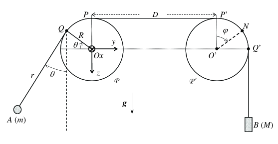
Figure 1: Schematisation of the system ${\cal S}=$ {pendulum-thread-pulleys-counterweight} representing SAM. The angle $\varphi$ locates the material point $N^{\prime}$ of the pulley ${\cal P}^{\prime}$.

${\cal S}$ is studied relative to the Galilean laboratory frame ${\cal R}=\left({O\,\mbox{\boldmath${e}$\unboldmath}_{x}\,\mbox{\boldmath${e}$\unboldmath}_{y}\,\mbox{\boldmath${e}$\unboldmath}_{z}}\right)$ whose origin $O$ is chosen to correspond to the centre of the pendulum pulley. Axis $Ox$ corresponds to the pulley revolution axis; axis $Oy$ is the horizontal direction defined by the pulley centres ($O$ and $O^{\prime}$), and oriented from $O$ toward $O^{\prime}$; finally, $Oz$ is chosen to correspond, for the sake of convenience, to the downward direction of the local earth gravity field ${g}$ (vertical).

Pendulum $A$ is characterized by its variable length $r=QA$, $Q$ being the geometrical point where the thread departs from the pulley, and by the angle $\theta$ formed by ${QA}$ and the downward vertical. Note that $\theta$ as represented in Figure 1 is a positive angle.

Vertical motion of the counterweight $B$ is described by its coordinate $z_{B}$, which can be related to the angular position $\varphi$ of any point $N$ on the pulleys, provided the thread does not slip on the pulley (in Figure 1, for the sake of clarity, $N$ is drawn on the pulley ${\cal P}^{\prime}$ associated to $B$ and thus labelled $N^{\prime}$). Indeed, under this assumption, when $B$ is falling down, pulleys are able to rotate in such a way that the velocity of any point of the pulleys (for instance $N^{\prime}$) is equal to the velocity of $B$. Hence:

$$\dot{z}_{B}=R\dot{\varphi}$$ (1)

Note the difference between the rotation angle $\varphi$ of the pulleys and $\theta$: the former defines the location of any material point on a pulley, whereas the latter defines the angular position of $A$, as well as that of the geometrical point of contact $Q$. This subtlety is due to the necessary mechanical description of contact in terms of three points [21]:

• the geometrical point of contact $Q$,

• the point $N$ of the pulley ${\cal P}$ and corresponding to $Q$ at time $t$,

• the point $K$ of the thread corresponding to $Q$ at time $t$.

Figure 2 displays the configuration. A similar problem can be found in [22].

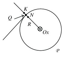
Figure 2: Description of the contact between a pulley and the thread with three points: $K$, $Q$, and $N$. At any time $t$, both $K$ and $N$ touch each other at $Q$. In the figure, these points are separated for the sake of clarity.

A physical way of understanding the difference between $\theta$ and $\varphi$ is to imagine the following situation. At initial time, assume that $Q$ and $N$ are superposed: $\theta=\theta_{0}$ and $\varphi=\varphi_{0}$ (Figure 3a). If $\theta$ is fixed and $B$ heads downwards with velocity $\dot{z}_{B}$, the absence of slippage of the thread on the pulleys implies that they rotate with angular velocity $\dot{\varphi}$ given by (1), meaning $N$ is moving while $Q$ remains fixed, and $r$ evolves from $r_{0}$ to $r$; at final time, $\varphi\neq\varphi_{0}$ (Figure 3b).

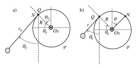
Figure 3: Evolution of point $N$ of the pulley ${\cal P}$ when $\theta$ is kept constant. The geometrical point of contact $Q$ is immobile and only $r$ evolves.

Since $L$ is supposed to be constant, $z_{B}$ is directly related to $r$, $D$, and the lengths $QP$ and $P^{\prime}Q^{\prime}$ corresponding to regions where the thread and the pulleys keep contact. Because

$$QP=R\left(\frac{\pi}{2}-\theta\right),\qquad P^{\prime}Q^{\prime}=\frac{\pi R}{2},$$

one has, precisely,

$$L=r+D+\pi R-R\theta+z_{B}.$$ (2)

Since $0=\dot{r}-R\dot{\theta}+\dot{z}_{B}$, it follows that

$$\dot{\varphi}=\frac{\dot{z_{B}}}{R}=\frac{R\dot{\theta}-\dot{r}}{R}.$$ (3)

Hence, ${\cal S}$ is a system with two degrees of freedom, for instance $\theta$ and $r$.

3 Equations of motion of SAM with pulleys

3.1 Equations of motion

Let us determine the equations of motion for SAM by taking into account the pulleys, as opposed to what has been assumed in previous theoretical studies [30, 27, 28, 31, 19, 29, 20, 35]. Indeed, their non-zero radii imply a likely change in position for $Q$, and the equally likely rotation of ${\cal P}$ and ${\cal P}^{\prime}$ around their respective revolution axes apparently deems their inertial momentum $I_{p}$ a significant dynamic parameter. Observations will confirm this – see Section 5.

Lagrange’s formalism is used to derive these equations. The kinetic energy of the system is expressed by:

$${\cal E}_{k}=\frac{1}{2}mv_{A}^{2}+\frac{1}{2}Mv_{B}^{2}+2\left(\frac{1}{2}I_{p}\dot{\varphi}^{2}\right)$$

The first term sums up the contribution by pendulum $A$, the second is relative to the counterweight $B$ and the third one corresponds to the rotation of the two pulleys. We have:

$$\mbox{\boldmath${v}$\unboldmath}_{A}=\frac{\mathrm{d}\mbox{\boldmath${OA}$\unboldmath}}{\mathrm{d}t}=\frac{\mathrm{d}\mbox{\boldmath${OQ}$\unboldmath}}{\mathrm{d}t}+\frac{\mathrm{d}\mbox{\boldmath${QA}$\unboldmath}}{\mathrm{d}t},$$

where $\mbox{\boldmath${OQ}$\unboldmath}=-R\cos\theta\,\mbox{\boldmath${e}$\unboldmath}_{y}-R\sin\theta\,\mbox{\boldmath${e}$\unboldmath}_{z}$ and $\mbox{\boldmath${QA}$\unboldmath}=-r\sin\theta\,\mbox{\boldmath${e}$\unboldmath}_{y}+r\cos\theta\,\mbox{\boldmath${e}$\unboldmath}_{z}$, hence in the Cartesian base $\left({O\,\mbox{\boldmath${e}$\unboldmath}_{x}\,\mbox{\boldmath${e}$\unboldmath}_{y}\,\mbox{\boldmath${e}$\unboldmath}_{z}}\right)$ we can write

$$\mbox{\boldmath${v}$\unboldmath}_{A}=\left(\begin{array}[]{c}{0}\\[5.0pt] {R\dot{\theta}\sin\theta-r\dot{\theta}\cos\theta-\dot{r}\sin\theta}\\[5.0pt] {-R\dot{\theta}\cos\theta-r\dot{\theta}\sin\theta+\dot{r}\cos\theta}\end{array}\right)$$

Similarly, $\mbox{\boldmath${v}$\unboldmath}_{B}=\mathrm{d}\mbox{\boldmath${OB}$\unboldmath}/\mathrm{d}t$ with $\mbox{\boldmath${OB}$\unboldmath}=z_{B}\,\mbox{\boldmath${e}$\unboldmath}_{z}$. Using (2), one gets

$$\mbox{\boldmath${v}$\unboldmath}_{B}=\dot{z}_{B}\,\mbox{\boldmath${e}$\unboldmath}_{z}=\left({R\dot{\theta}-\dot{r}}\right)\,\mbox{\boldmath${e}$\unboldmath}_{z}.$$

Finally, using (3) and introducing the effective total mass of the system

$$M_{t}=M+m+\frac{2I_{p}}{R^{2}},$$

we get

$${\cal E}_{k}=\frac{1}{2}M_{t}(R\dot{\theta}-\dot{r})^{2}+\frac{1}{2}mr^{2}\dot{\theta}^{2}.$$

This expression is similar to that obtained when neglecting the pulleys, except that:

• the total mass is now different from $M+m$ by the term $2I_{p}/R^{2}$ conveying the rotation of the pulleys;

• the counterweight influences pendulum $A$ through its length $r$ and the winding of the rope on the associated pulley. The latter influence is considered in the term $R\dot{\theta}$.

Potential energy is only due to the Earth’s local gravity field. Dropping an irrelevant additional constant term, we have:

$${\cal E}_{p,g}=-m\mbox{\boldmath${g}$\unboldmath}\cdot\mbox{\boldmath${OA}$\unboldmath}-M\mbox{\boldmath${g}$\unboldmath}\cdot\mbox{\boldmath${OB}$\unboldmath}=-mgz_{A}-Mgz_{B},$$

so that

$${\cal E}_{p,g}=mg(R\sin\theta-r\cos\theta)+Mg(r-R\theta).$$

The Lagrangian ${\cal L}(r,\theta,\dot{r},\dot{\theta})={\cal E}_{k}-{\cal E}_{p,g}$ of the system is thus:

$${\cal L}(r,\theta,\dot{r},\dot{\theta})=\frac{1}{2}M_{t}(R\dot{\theta}-\dot{r})^{2}+\frac{1}{2}mr^{2}\dot{\theta}^{2}-gr(M-m\cos\theta)-gR(m\sin\theta-M\theta),$$

from which one deduces the conjugate momenta $p_{r}$ and $p_{\theta}$ associated to $r$ and $\theta$ respectively:

$$p_{r} = \frac{\partial{\cal L}}{\partial\dot{r}}=-M_{t}(R\dot{\theta}-\dot{r})$$

$$p_{\theta} = \frac{\partial{\cal L}}{\partial\dot{\theta}}=M_{t}R(R\dot{\theta}-\dot{r})+mr^{2}\dot{\theta}=-Rp_{r}+mr^{2}\dot{\theta}$$

The SAM Hamiltonian is, in this case, by definition:

$${\cal H}={\cal E}_{k}+{\cal E}_{p,g},$$

or else, expressed in terms of $p_{r}$ and $p_{\theta}$:

$${\cal H}(r,\theta,p_{r},p_{\theta})=\frac{1}{2}\left[\frac{p_{r}^{2}}{M_{t}}+\frac{(p_{\theta}+Rp_{r})^{2}}{mr^{2}}\right]+gr(M-m\cos\theta)+gR(m\sin\theta-M\theta).$$ (4)

Equations of motion follow from the Hamilton’s equations:

$${\dot{p_{r}}=-\frac{\partial{\cal H}}{\partial r}\qquad\hbox{and}\qquad\dot{p_{\theta}}=-\frac{\partial{\cal H}}{\partial\theta}},$$

yielding

$$\left\{\begin{array}[]{rcl}\mu_{t}(\ddot{r}-R\ddot{\theta})&=&r\dot{\theta}^{2}+g(\cos\theta-\mu)\\ r\ddot{\theta}&=&-2\dot{r}\dot{\theta}+R\dot{\theta}^{2}-g\sin\theta\end{array}\right.$$ (5)

with $\mu=M/m$ and $\mu_{t}=M_{t}/m=1+\mu+\left(2I_{p}/mR^{2}\right)$.

3.2 A more physical way to obtain equations of motion

An alternative method can be used in order to derive equations of motion (5). The second of these is obtained by applying the angular momentum theorem at the mobile point $Q$ in order to cancel reaction force at this contact point [21]:

$$\frac{\mathrm{d}\mbox{\boldmath${L}$\unboldmath}_{Q}}{\mathrm{d}t}+\mbox{\boldmath${v}$\unboldmath}_{Q}\times m\mbox{\boldmath${v}$\unboldmath}_{A}=\mbox{\boldmath${QA}$\unboldmath}\times m\mbox{\boldmath${g}$\unboldmath},$$

where $\mbox{\boldmath${L}$\unboldmath}_{Q}=\mbox{\boldmath${QA}$\unboldmath}\times m\mbox{\boldmath${v}$\unboldmath}_{A}=mr^{2}\dot{\theta}\,\mbox{\boldmath${e}$\unboldmath}_{x}$ and

$$\mbox{\boldmath${v}$\unboldmath}_{Q}=\frac{R\dot{\theta}}{AQ}\mbox{\boldmath${AQ}$\unboldmath},\qquad\mbox{\boldmath${v}$\unboldmath}_{A}=\frac{r\dot{\theta}}{OQ}\mbox{\boldmath${OQ}$\unboldmath}+\frac{\dot{r}}{QA}\mbox{\boldmath${QA}$\unboldmath}.$$

We obtain $r\ddot{\theta}=-2\dot{r}\dot{\theta}+R\dot{\theta}^{2}-g\sin\theta$. Taking this into account, the first equation in (5) comes from the conservation of mechanical energy in SAM:

$${\cal E}_{m}=\frac{1}{2}M_{t}(R\dot{\theta}-\dot{r})^{2}+\frac{1}{2}mr^{2}\dot{\theta}^{2}+mg(R\sin\theta-r\cos\theta)-Mg(R\theta-r)=C$$

$C$ being a real constant, after derivation with respect to $t$.

3.3 Comparison with previous studies

Without any pulley influence, i.e. pulley inertial momentum $I_{p}=0$ and pulley radius $R=0$, we recover the equations obtained by [30]:

$$\left\{\begin{array}[]{rcl}(1+\mu)\ddot{r}&=&r\dot{\theta}^{2}+g(\cos\theta-\mu)\\ r\ddot{\theta}&=&-2\dot{r}\dot{\theta}-g\sin\theta\end{array}\right.$$ (8)

Obviously, if there is no oscillatory motion ($\theta=0$), the well-known simple Atwood machine [5] is recovered:

$$M_{t}\ddot{r}=g(m-M)$$ (9)

4 Description of the experimental apparatus

A physical prototype for SAM has been built using two identical pulleys, a nylon thread, a brass ball as a pendulum and a set of different hook masses acting as counterweights. The pendulum and the chosen counterweight are linked together by the nylon thread placed around the pulleys. A photo of SAM is displayed in Figure 4.

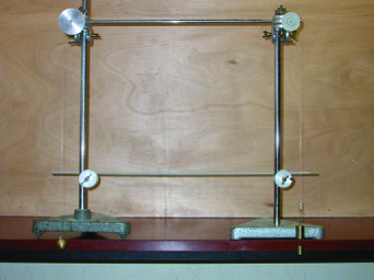
Figure 4: Photo of the Swinging Atwood Machine (SAM): a pendulum (on the left) and a counterweight (on the right), linked together by a nylon thread.

4.1 About the pendulum and the counterweight

Each mass in the experimental device has been measured with a precision scale of $0.01\,\mathrm{g}$ of accuracy. The pendulum is a brass ball with a $30\,\mathrm{mm}$ diameter and a mass $m=118.36\,\mathrm{g}$. The picture of the pendulum in Figure 5a also exhibits a paper clip and the nylon thread, the latter being solidly tied to the brass ball and the paper clip.

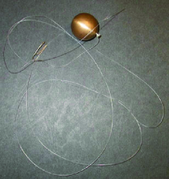
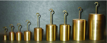
(a)	(b)

Figure 5: (a) Brass ball (pendulum), nylon thread and paper clip (b) Set of hook masses used in the experiment (counterweight). From left to right: $10\,\mathrm{g}$, $20\,\mathrm{g}$, $20\,\mathrm{g}$, $50\,\mathrm{g}$, $100\,\mathrm{g}$, $200\,\mathrm{g}$, $200\,\mathrm{g}$, $500\,\mathrm{g}$, $1000\,\mathrm{g}$.

The paper clip is secured to the hook of the chosen counterweight, in turn picked out from nine hook masses whose measured values are $M=10.01\,\mathrm{g}$, $20.02\,\mathrm{g}\,(\times 2)$, $50.05\,\mathrm{g}$, $100.10\,\mathrm{g}$, $200.22\,\mathrm{g}\,(\times 2)$, $500.51\,\mathrm{g}$, and $1000.10\,\mathrm{g}$ (Figure 5b). The relative difference between these values and those engraved in each hook mass is $0.1\,\mathrm{\%}$; thus, with respect to the orders of magnitude of the different masses involved in the experimental device, this difference can be neglected. The values considered are therefore presumed to be those indicated on the hook mass themselves, namely $M=10\,\mathrm{g}$, $20\,\mathrm{g}\,(\times 2)$, $50\,\mathrm{g}$, $100\,\mathrm{g}$, $200\,\mathrm{g}\,(\times 2)$, $500\,\mathrm{g}$, and $1000\,\mathrm{g}$. Henceforth, and for the sake of linguistic simplicity, these hook masses will be called “counterweights”, although weight and mass are different notions, however related. This set enables varying the counterweight mass from $10\,\mathrm{g}$ (one mass) to $2\,100\,\mathrm{g}$ (addition of all the masses) with a step of $10\,\mathrm{g}$ by hooking several masses together. Among these hook masses, one is hung on the nylon thread by means of the paper clip, whose measured mass is $0.37\,\mathrm{g}$. It is interesting to note that, by a fortunate coincidence, the mass of the paper clip is equal, with a $0.01\,\mathrm{g}$ difference, to $0.36\,\mathrm{g}$, i.e. the mass of the brass ball minus $118\,\mathrm{g}$. Therefore, the mass of the brass ball can be taken as equal to $118\,\mathrm{g}$ and the mass of the paper clip can be ignored. Finally, we get, for the pendulum and the counterweight, respectively: $m=118\,\mathrm{g}$ and $10\,\mathrm{g}\leq M\leq 2100\,\mathrm{g}$.

4.2 About the nylon thread and the pulleys

The thread (Figure 5a) ensures a mechanical coupling between the pendulum and the counterweight through the two pulleys. The length of the thread is about one meter and its measured mass of $0.10\,\mathrm{g}$ is negligible compared to the other masses involved. In addition, the nylon thread is assumed inextensible. During experimentation, no thread breaking has been reported.

Pulleys used are shown in photos of Figure 6. They are made up of two parts: an internal, immobile one bound to the revolution axis, and a mobile, external one liable to rotate around this axis. These two pulley components are uncoupled through a ball bearing which, moreover, reduces mechanical energy dissipation by friction. Pulley radius is $R=2.5\,\mathrm{cm}$ and that of the motionless part is $1\,\mathrm{cm}$. Pulley ${\cal P}$, associated to the pendulum, has been modified in order to make its groove deeper. Indeed, during the first experimentations we observed that the thread could rapidly exit the groove because of the pendulum motion. To avoid this, which could by the way be dangerous, two metallic plates were added and fixed to the pulley in order to increase by $1\,\mathrm{cm}$ the depth of the groove (Figures 6a and  6b). It is worth noting that the plates are fixed to the immobile part of the pulley and are in no way in contact with the mobile one. The motion of the latter one is thus not affected by such a modification: hence, from a mechanical point of view, the resulting pulley is identical to the original one.

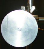
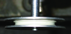
(a)	(b)
(c)	(d)

Figure 6: Photos of the two pulleys. (a) Pulley ${\cal P}$, front view: a metallic plate is added which hides the internal part and the ball bearing of the original pulley. (b) Pulley ${\cal P}$, top view: the groove is made deeper by $1\,\mathrm{cm}$ with the additional plate; the original pulley is easily recognizable between the two plates. (c) Pulley ${\cal P}^{\prime}$, front view: the ball bearing uncouples the immobile internal part and the mobile external one (d) Pulley ${\cal P}^{\prime}$, top view: photograph of the axis of revolution and the groove of the pulley. Moreover, the two pulleys are distant enough from one another to avoid a pendulum-counterweight collision during the motion.

4.3 Strengthening of the apparatus

Figure 4 also features two horizontal metallic rods binding the two feet of SAM. Their role is to reinforce the machine. Indeed, due to considerable stress involved in the pendulum and counterweight motions, the orientation of the two pulleys, as well as the arbitrary distance $D=57.5\,\mathrm{cm}$ between them, can change; thus, it could be dangerous not to strengthen the whole device. The lower metallic rod is solidly fixed to the feet while the upper one is solidly fixed to the revolution axes of the pulleys. Consequently, we ensured a constant distance between the pulleys whose axes keep a constant direction; in virtue of such a construction, SAM is solid and operational.

5 Motion of the pendulum: experimental results

5.1 Experimental measure of $I_{p}$

The presence of the inertial momentum $I_{p}$ of a pulley in (5) renders an experimental determination thereof necessary. This measure was made using a simple Atwood machine where the heavier mass ($M=130\,\mathrm{g}$) fell down from a convenient height $h=1.66\,\mathrm{m}$; the lighter mass (the brass ball) being $m=118\,\mathrm{g}$. Using equation (9), one gets:

$$I_{p}=R^{2}\left[\frac{(M-m)g(\Delta t)^{2}}{2h}-(M+m)\right].$$

where $\Delta t$ is the fall duration. Through a set of ten measures with a chronometer of $0.01\,\mathrm{s}$ of accuracy, the mean fall duration found is $\left\langle\Delta t\right\rangle=2.70\pm 0.01\,\mathrm{s}$. $\left\langle I_{p}\right\rangle=6.85\times 10^{-6}\,\mathrm{kg\cdot m^{2}}$ ensues. Concerning the value of $I_{p}$, errors are due to the measure of both $\Delta t$ and the positions of $M$ at the initial and final times – that is, the determination of $h$. Uncertainties are mainly due to the determination of the final time, which must correspond to the falling distance $h$ as precisely as possible; initial and final positions are determined with an error of $0.1\,\mathrm{cm}$, which compared to the value of $h$ can be neglected. Consequently, uncertainties in position determinations are disregarded and the error in the measure of $I_{p}$ can be reasonably associated to the uncertainty in $\Delta t$ ($0.4\hbox{ \%}$). Thus, precision on $I_{p}$ is twice that of $\Delta t$, hence about $1\hbox{ \%}$; absolute uncertainty is thus $0.07\times 10^{-6}\,\mathrm{kg\cdot m^{2}}$. Therefore, we can write:

$$I_{p}=(6.85\pm 0.07)\times 10^{-6}\,\mathrm{kg\cdot m^{2}}\qquad\hbox{or}\qquad I_{p}=6.85\times 10^{-6}\,\mathrm{kg\cdot m^{2}}\pm 1\hbox{ \%}.$$

5.2 Experimental results

The motion of the pendulum has been filmed for various $\mu$-values and initial conditions $(r_{0}\,;\,\theta_{0})$. Then, using the “Synchronie” software and focusing on each film image by image, a pointer enabled us to pick up pendulum positions and record them. Such a process is necessarily a source of errors, as it is sometimes difficult to locate the pendulum exactly, especially if velocity is high. The errors introduced by such a procedure are not simple to estimate. However, trajectories have been correctly recorded, as comparisons with numerically-simulated theoretical results will show (see Section 6).

5.2.1 Case $\mu_{\mathrm{theo}}=3$

Since previous studies focused mainly on the particular and theoretical case $\mu_{\mathrm{theo}}=3$, this was the first one we experimentally addressed. In fact, the masses available only allowed us to approach $\mu_{\mathrm{theo}}$: with $m=118\,\mathrm{g}$ and $M=350\,\mathrm{g}$ one obtains $\mu_{\mathrm{exp}}=2.966$, which is the closest value to $\mu_{\mathrm{theo}}$. The sampling time step has been $67\,\mathrm{ms}$. Motion has been researched for four different initial conditions $(r_{0}\,;\,\theta_{0})$=$(0.649\,;\,53.5)$, $(0.710\,;\,66.5)$, $(0.854\,;\,68.3)$ and $(0.867\,;\,51.1)$; $r_{0}$ is in meters, $\theta_{0}$ in degrees. The motion of the pendulum presents the same pattern and characteristics for all these conditions, so only the trajectory for the first initial conditions is shown in Figure 7a. All in all, $359$ sampling times have been recorded. The pendulum has a planar revolving trajectory around the pulley and presents an asymmetry with respect to the vertical direction. Note that the pendulum becomes closer and closer to the pulley as a consequence of dissipative phenomena and is bound to end up knocking against it. Phenomena qualifying as dissipative are, to our knowledge: the friction between the thread and the pulley, the air friction on the pendulum and the counterweight as well as friction inside the ball bearing. Evolutions of the length of the pendulum $r$ and angle $\theta$ are displayed in Figure 7b and Figure 7c respectively. The asymmetry of the trajectory and dissipation are observable in the evolution of $r$ since this variable exhibits different minimal and maximal amplitudes which decrease in function of time $t$.

The Fourier analysis (non-displayed) of the data shows that, for the behaviour of $\theta$, the most relevant harmonic is the constant term, followed by harmonics $7$, $6$ and $8$. They account, respectively, for $0.401$, $0.311$, $0.117$, and $0.091$ of the total variation. Of course, the contributions of harmonics $6$ and $8$ are due to leakage of the $7^{\mathrm{th}}$ one. The amplitude of the $6^{\mathrm{th}}$ harmonic is larger than that of the $8^{\mathrm{th}}$, showing that the true dominant average frequency is slightly less than $7$ times the basic frequency. From the number of data and the sampling step time, a basic frequency of $0.042\,\mathrm{Hz}$ follows. Hence, an average value of the dominant frequency can be estimated to be equal to $0.294\,\mathrm{Hz}$. However, as is clear by looking at the maxima of the angle, the frequency changes with time. The spacing between successive maxima takes the approximate values $3.820\,\mathrm{s},3.909\,\mathrm{s},3.379\,\mathrm{s},3.311\,\mathrm{s},3.173\,\mathrm{s},2.780\,\mathrm{s}$, and $2.643\,\mathrm{s}$. Hence, the instantaneous frequency changes from about $0.262\,\mathrm{Hz}$ to about $0.378\,\mathrm{Hz}$. The explanation is simple: the dissipation reduces the energy and the length of the pendulum becomes shorter, increasing the frequency.

For the radius, the major contribution comes from the constant term, followed by harmonics $13$ and $7$. They account for $0.810,0.037$, and $0.026$ of the total variation. Comparing the plot of $r$ as a function of time with that of $\theta$, one can see a doubling in the number of maxima. The explanation is simple: largest maxima occur at the left part of the plot of the orbit. Then, a minimum is reached when $\theta=-\pi$ (i.e., upwards), followed by a maximum to the right, and a new minimum at $\theta=-\pi$ to reach a larger maximum on the left. The spacing between successive larger maxima of $r$ is very close to the one observed for $\theta$. As mentioned, the largest non-constant harmonics are the $13^{\mathrm{th}}$ and the $7^{\mathrm{th}}$, not in a 2-to-1 ratio. This is related to the fact that the “best” estimate of the main frequency for $\theta$ is slightly less than $7$ times the basic frequency. The closest integer to the double would be $13$ rather than 14.

The decrease in energy can be calculated as follows. From the experimental data, the values of $\dot{r}$ and $\dot{\theta}$ can be computed. For that, we have used two independent methods. The first one is simply numerical differentiation with a central formula. The second one aims at filtering errors in the data as well. A Discrete Fourier Transform has been computed and harmonics up to order $32$ have been retained. Then, it is possible to check that the reconstruction agrees quite well with the initial data and one can compute the values of $\dot{r}$ and $\dot{\theta}$ using these Fourier expansions. To prevent leakage due to the fact that the data at the ends of the interval are quite different (Figs. 7b and c), which originates the well-known $O(1/n)$ decrease of the order of magnitude of the $n^{\mathrm{th}}$ harmonic, different procedures have been used, but the results are essentially the same. They also show a reasonable agreement using the first and second methods.

Figure 7: Case $\mu_{\mathrm{exp}}=2.966$ with initial conditions $r_{0}=0.649\,\mathrm{m}$ and $\theta_{0}=53.5^{\circ}$. (a) Experimental positions (black crosses) and interpolated pendulum trajectory (solid line). The Cartesian coordinates of the initial position are $y=-0.54\,\mathrm{m}$ and $z=0.37\,\mathrm{m}$ and those of the final position are $y=0.02\,\mathrm{m}$ and $z=-0.05\,\mathrm{m}$. The pulley is represented by the circle whose centre is at the origin of coordinates $(0\,;\,0)$. (b) Experimental positions (black crosses) and interpolated curve (solid line) for the evolution of $r$. (c) Same as (b) but for the angle $\theta$.

When $\dot{r}$ and $\dot{\theta}$ are available, one can compute $p_{r}$ and $p_{\theta}$ and subsequently the value of the energy. The values for which $\theta$ reaches a maximum (i.e., on the left of Figure 7a) are shown in Figure 8. The rate of decrease of the energy is about $0.037\,\mathrm{J\cdot s^{-1}}$.

Figure 8: Values of the energy (crosses) occurring when $\theta$ reaches a maximum at the left part of Figure 7a. We have also displayed the function ${\cal E}_{m}=1.723-0.037\,t$.

5.2.2 Case $\mu_{\mathrm{theo}}=1.5$

The experimental value of $\mu$ closest to $\mu_{\mathrm{theo}}=1.5$ is $\mu_{\mathrm{exp}}=1.525$, given by $M=180\,\mathrm{g}$. Proceeding as in the above case allows us to retrieve the experimental trajectory and the evolution of the degrees of freedom. In this case, time step is $40\,\mathrm{ms}$. Two initial conditions have been considered: $(r_{0}\,;\,\theta_{0})$=$(0.484\,\mathrm{m}\,;\,87.0^{\circ})$ and $(0.621\,\mathrm{m}\,;\,87.7^{\circ})$. Since they produce the same dynamic behaviour, only the first one is displayed (Figures 9a, 9b and 9c respectively). A slight asymmetric trajectory with respect to the vertical direction and an evolution of $\theta$ close to periodic with a period around $1.1-1.2\,\mathrm{s}$ can be observed. For the evolution of $r$, asymmetry and slight dissipation are also observed.

A study similar to that of $\mu_{\mathrm{exp}}=2.966$ is performed. The main contribution to the Fourier analysis of $\theta$ comes from harmonic number $7$ which accounts for $0.912$ of the total variation with a frequency of approximately $0.875\,\mathrm{Hz}$, although a better value for the average frequency seems to be $0.89\,\mathrm{Hz}$. Harmonics $14$ and $21$ also play a relevant role. As we did for $\mu_{\mathrm{exp}}=2.966$, we can consider the spacing between successive maxima of $\theta$ which takes the values $1.125\,\mathrm{s}$, $1.119\,\mathrm{s}$, $1.114\,\mathrm{s}$, $1.110\,\mathrm{s}$, $1.156\,\mathrm{s}$, $1.133\,\mathrm{s}$ and $1.063\,\mathrm{s}$, showing a decreasing trend with irregularities.

For $r$, the largest harmonic is the constant term which accounts for $0.971$ of the signal. If we skip this term, harmonics $7$, $14$ and $3$ are clearly seen. They contribute to $0.30$, $0.29$, and $0.14$ of the signal minus the constant part.

Figure 9: Same as Figure 7 but for $\mu_{\mathrm{exp}}=1.525$ and initial conditions $r_{0}=0.484\,\mathrm{m}$ and $\theta_{0}=87.0\,\mathrm{{}^{\circ}}$. In (a), the Cartesian coordinates of the initial position are $y=-0.485\,\mathrm{m}$ and $z=0$ ; for the final position, one has $y=-0.330\,\mathrm{m}$ and $z=0.195\,\mathrm{m}$. The origin $(0\,;\,0)$ corresponds to the centre of the pulley (not represented).

The decrease of the energy as a function of time has been displayed in Figure 10, this time using the values of the energy computed at the minima of $\theta$, on the right part of Figure 9a. Now the rate of decrease is about $0.024\,\mathrm{J\,s^{-1}}$. In this case, using the filtered Fourier methods gives better results, because of the large changes in position with a time step of $40\,\mathrm{ms}$.

Figure 10: Values of the energy (crosses) occurring when $\theta$ reaches a minimum at the right part of Figure 9a. We have also displayed the function ${\cal E}_{m}=0.751-0.024\,t$.

5.2.3 An unbounded case: $\mu_{\mathrm{theo}}=1$

In this situation, the experimental value of $\mu$ is $\mu_{\mathrm{exp}}=1.017$ and three initial conditions have been considered: $r_{0}=0.120\,\mathrm{m}$, $0.263\,\mathrm{m}$ and $0.477\,\mathrm{m}$ for $\theta_{0}=77.9^{\circ}$. Again, trajectories present the same pattern, so only one is shown (Figure 11a). They are characterized by an increase in $r$ and $\theta$ oscillations around the vertical $(\theta=0)$ with a decreasing amplitude of $\theta$ (Figures 11b and c respectively). In Figure 11b, $r$ appears to approach a linear increase in time: $r=v_{z}t$ where $v_{z}$ is the velocity along the vertical.

Figure 11: Same as Figure 7 but for $\mu_{\mathrm{exp}}=1.017$ and initial conditions $r_{0}=0.120\,\mathrm{m}$ and $\theta_{0}=77.9\,\mathrm{{}^{\circ}}$. In (a), the Cartesian coordinates of the initial position are $y=-0.122\,\mathrm{m}$ and $z=0$ ; for the final position, one has $y=-0.116\,\mathrm{m}$ and $z=1.167\,\mathrm{m}$. The origin $(0\,;\,0)$ corresponds to the centre of the pulley (not represented).

6 Numerical solution of SAM equations of motion

6.1 Theoretical trajectories

Equations of motion (5) have been numerically integrated for the same initial conditions and values of the parameter $\mu$ as above in order to compare the theoretical trajectories, displayed in Figure 12, with the experimental ones. Computation of the theoretical trajectories has been performed by using both a Taylor integration method and a variety of Runge-Kutta methods of different orders with step-size control to integrate the equations of motion.

From a general point of view, the theoretical trajectories seem quite similar to the experimental ones. However, some slight differences can be detected. Firstly, it is obvious that dissipative phenomena, though experimentally reduced, play a non-negligible role since convergence of the pendulum towards the pulley for the first case (Fig. 7b), decrease of $r$ for the second one (Fig. 9b) and relatively slow increasing of $r$ for the third one (Fig. 11b) are clearly associated to energy dissipation. Friction will be studied a bit further in Subsection 6.3 and much more in future works. Secondly, it must be said that for the case $\mu_{\mathrm{exp}}=2.966$ the pendulum touches the nylon thread at each revolution, an effect which could be included into the equations of motion through a dissipative term; however, it seems quite difficult to introduce such an effect in a realistic manner.

An important point concerns the comparison between these trajectories and those of [30]. For the first case for instance, Tufillaro’s trajectories are symmetrical with respect to the vertical direction, as opposed to the above ones (Figures 7a and  12a). Clearly, this asymmetry is due to the influence of the pulleys.

6.2 Influence of the pulleys on the motion

Pulleys can influence the motion of SAM through their dimension (since radius $R\neq 0$) and their rotation (since $I_{p}\neq 0$).

6.2.1 Influence of the radius: $\mu_{\mathrm{exp}}=2.966$

Figure 14 sketches the trajectory for $\mu_{\mathrm{exp}}=2.966$ when $I_{p}=0$ for different values of increasing $R$; i.e. the pendulum pulley $\cal{P}$ has a non-negligible radius but pulleys are not allowed to rotate. The first figure corresponds to the symmetrical Tufillaro trajectory $(R=0,I_{p}=0)$. Ostensibly, the larger $R$ is, the more significant the asymmetry becomes; for $R=5\,\mathrm{cm}$, the pendulum hits the pulley before completing one revolution.

6.2.2 Influence of the inertial momentum: $\mu_{\mathrm{exp}}=2.966$

Figure 14 sketches the trajectory for $\mu_{\mathrm{exp}}=2.966$ for increasing values of $I_{p}$ with a value of pulleys radius taken to the real value $R=2.5\,\mathrm{cm}$. The trajectory of the pendulum is visibly modified: it describes more irregular trajectories and fills more space as $I_{p}$ increases.

Figure 12: Numerical trajectories obtained by solving equations of motion (5). (a) $\mu_{\mathrm{exp}}=2.966$ and for the same initial conditions as Figure 7a. (b) $\mu_{\mathrm{exp}}=1.525$ and for the same initial conditions as Figure 9a. (c) $\mu_{\mathrm{exp}}=1.017$ and for the same initial conditions as Figure 11a.

Figure 13: Theoretical trajectories of the pendulum with fixed pulleys of different radii $R$ for $\mu_{\mathrm{exp}}=2.966$ and initial condition $(r_{0}\,;\,\theta_{0})$=$(0.649\,\mathrm{m}\,;\,53.5^{\circ})$. (a) $R=0$, (b) $R=2.5\,\mathrm{cm}$, (c) $R=4\,\mathrm{cm}$ and (d) $R=5\,\mathrm{cm}$. In the latter subplot, the pulley has been represented by the circle whose centre is at the origin of coordinates in order to see the collision between the pendulum and the pulley.

Figure 14: Theoretical trajectories of the pendulum with pulleys of radius $R=2.5\,\mathrm{cm}$ and different inertial momenta $I_{p}$ for $\mu_{\mathrm{exp}}=2.966$ and initial condition $(r_{0}\,;\,\theta_{0})$=$(0.649\,\mathrm{m}\,;\,55.7^{\circ})$. (a) $I_{p}=0$; this subplot which is the same as Figure 14b has been repeated for the sake of clarity, (b) $I_{p}=6.85\times 10^{-6}\,\mathrm{kg\cdot m^{2}}$, (c) $I_{p}=13.70\times 10^{-6}\,\mathrm{kg\cdot m^{2}}$ and (d) $I_{p}=27.40\times 10^{-6}\,\mathrm{kg\cdot m^{2}}$.

Figure 15: Theoretical trajectories of the pendulum with fixed pulleys of different radii $R$ for $\mu_{\mathrm{exp}}=1.525$ and initial condition $(r_{0}\,;\,\theta_{0})$=$(0.484\,\mathrm{m}\,;\,87.0^{\circ})$. (a) $R=0$, (b) $R=2.5\,\mathrm{cm}$, (c) $R=5\,\mathrm{cm}$ and (d) $R=10\,\mathrm{cm}$.

Figure 16: Theoretical trajectories of the pendulum with pulleys of radius $R=2.5\,\mathrm{cm}$ and different inertial momenta $I_{p}$ for $\mu_{\mathrm{exp}}=1.525$ and initial condition $(r_{0}\,;\,\theta_{0})$=$(0.484\,\mathrm{m}\,;\,87.0^{\circ})$. (a) $I_{p}=0$; this subplot which is the same as Figure 16b has been repeated for the sake of clarity, (b) $I_{p}=6.85\times 10^{-6}\,\mathrm{kg\cdot m^{2}}$, (c) $I_{p}=13.70\times 10^{-6}\,\mathrm{kg\cdot m^{2}}$ and (d) $I_{p}=54.80\times 10^{-6}\,\mathrm{kg\cdot m^{2}}$.

6.2.3 Influence of the pulleys: $\mu_{\mathrm{exp}}=1.525$

In this case, results of variations in $R$ with $I_{p}=0$ (Figure 16) and $I_{p}$ variations for $R=2.5\,\mathrm{cm}$ (Figure 16) are similar in that trajectories are modified more visibly as $R$ and $I_{p}$ increase. However, the influence of $I_{p}$ and $R$ on SAM motion depends on the value of $\mu$ considered. If $R$ increases, the pulleys being fixed, the brass ball ends up hitting the pulley but asymmetry does not becomes more and more important. If $I_{p}$ increases, pulley dimensions being fixed, the pendulum evolves in a much more limited space.

6.3 Poincaré maps and rotation number

To have a global view of the dynamics of SAM, we have computed Poincaré maps ${\cal P}_{m}$ on suitable Poincaré sections. We note that the Hamiltonian (4) is not $2\pi$-periodic because of the linear term in $\theta$. Be that as it may, our Poincaré section $\Sigma$ defining ${\cal P}_{m}$ is given by the coiling of $\theta$ through multiples of $2\pi$, with $\dot{\theta}>0.$ But, contrarily to SAM without pulleys ([27]), one has to distinguish between cuts through different multiples of $2\pi$. Plus, one can not superimpose the different sheets.

Some types of “escape” can occur. The main source thereof is $r$ going to zero. Other relevant sources of escape are $r$ increasing too much or $\left|\theta\right|$ becoming too large. All orbits leading to some of these escapes are deleted.

To compare with the experiments, we present some examples for $M=350\,\mathrm{g}$ and $M=180\,\mathrm{g}$. As levels of energy, one has taken the values corresponding to the experiments described in 5.2.1 and 5.2.2, that is, $(r_{0}\,;\,\theta_{0})$=$(0.649\,\mathrm{m}\,;\,53.5^{\circ})$ and $(r_{0}\,;\,\theta_{0})$=$(0.484\,\mathrm{m}\,;\,87.0^{\circ})$, respectively, with zero initial velocity. Given $r$, $p_{r}$ in $\Sigma$ and $\theta=0$, the value of $p_{\theta}$ is recovered from the energy level. Figure 17 shows some results. All these massive computations use Taylor integration methods, in order to ensure a very good conservation of the energy (see, e.g., [24]).

The top left plot corresponds to $M=350\,\mathrm{g}$, leaving $\Sigma$ with $p_{r}>0$. The points on $\Sigma$ with $p_{r}<0$ correspond to cuts through $\theta=-2\pi$, in agreement with the description of motion in 5.2.1. To produce the Poincaré map, we first computed the periodic orbit as a fixed point in $\Sigma\cap\left\{p_{r}>0\right\}$. The approximate values $(r^{*}\,;\,p_{r}^{*})$ of the fixed point are $(0.332814\,\mathrm{m}\,;\,0.554330\,\mathrm{kg\cdot m\cdot s^{-1}})$. This periodic orbit can also be obtained by starting the motion from rest at $(r_{0}\,;\,\theta_{0})\approx(0.61316\,\mathrm{m}\,;\,64.032^{\circ})$, not too far from the values used in the experiment. The curve drawn with large dots around the periodic orbit shows the iterates of ${\cal P}_{m}$ corresponding to the data used in the experiment. It is clear that the theoretical, non-dissipative, motion seems to be in a $2\mathrm{D}$ torus, but numerical computations can never exclude the possibility of having a periodic orbit with very long period or a tiny chaotic zone. The intersection of this torus with $\theta=-2\pi$ is also shown in the region $p_{r}<0$. The asymmetry is ostensible in the plot, and is due to the effect of the pulleys. To produce the full plot, we have taken initial conditions on $\Sigma$ with $r=r^{*}$ and different values of $p_{r}$ starting at $p_{r}^{*}$. From some value of $p_{r}$ onwards, iterates escape. We do not exclude the presence of tiny islands outside the last invariant curve shown.

For the sake of completeness, we show in the top right plot the Poincaré iterates leaving $\Sigma$ in the region $\left\{p_{r}<0\right\}$. Points appearing in $\left\{{p_{r}>0}\right\}$ are on the sheet $\left\{{\theta=2\pi}\right\}$. The fixed point in $\left\{{p_{r}<0}\right\}$ is approximately $(0.383367\,\mathrm{m}\,;\,-0.620020\,\mathrm{kg\cdot m\cdot s^{-1}})$.

Figure 17: Iterates of Poincaré maps for $M=350\,\mathrm{g}$ (top row) and $M=180\,\mathrm{g}$ (bottom plot) on the levels of energy of the physical experiments described in the text. The variables $(r\,;\,p_{r})$, as usual in $\,\mathrm{m}$ and $\,\mathrm{kg\cdot m\cdot s^{-1}}$, respectively, are shown for $\theta=0$ (mod $2\pi$) and $\dot{\theta}>0$. On the top left plot, the points leave the section with $p_{r}>0$ and $\theta=0$, and those with $p_{r}<0$ are in $\theta=-2\pi$. On the right top row, top initial points are in $\theta=0$ with $p_{r}<0$, and those showing in $p_{r}>0$ have $\theta=2\pi$. On the bottom plot, all intersections occur at $\theta=0$. The thick curves are the intersections of the theoretical $2\mathrm{D}$ tori corresponding to the physical experiments with the section $\Sigma$.

The bottom plot corresponds to $M=180\,\mathrm{g}$. In that case, only intersections having $\theta=0$ are found. The fixed point is $(r^{*}\,;\,p_{r}^{*})\approx(0.356386\,\mathrm{m}\,;\,0.008848\,\mathrm{kg\cdot m\cdot s^{-1}})$, which can also be obtained leaving from $(r_{0}\,;\,\theta_{0})=(0.53313\,\mathrm{m}\,;\,78.596^{\circ})$, again not too far from the values used in the experiment. As before, the curve drawn with large points around the periodic orbit would be the one obtained for the physical experiment without dissipation and, as expected, denotes motion on a $2\mathrm{D}$ torus.

A useful tool to understand the dynamics of Area-Preserving Maps and, in particular, Poincaré maps such as the ones displayed, is the rotation number $\rho$ for the map restricted to invariant curves. Despite the fact that the rotation number still exists for periodic orbits of ${\cal P}_{m}$ and for the eventual islands around them (thereupon being rational), it is not defined, in general, for orbits with chaotic dynamics. The method used for the computation is topological and based on the order of the arguments of the iterates with respect to the central fixed point $(r^{*}\,;\,p_{r}^{*})$ of ${\cal P}_{m}$. The procedure computes two estimates $\rho_{\mathrm{inf}}$ and $\rho_{\mathrm{sup}}$ such that $\rho_{\mathrm{inf}}\leq\rho\leq\rho_{\mathrm{sup}}$. If for some orbit one has $\rho_{\mathrm{inf}}>\rho_{\mathrm{sup}}$ this proves $\rho$ not defined. If the number of ${\cal P}_{m}$ iterates is $N$, the typical errors, when $\rho$ exists, are $O\left({N^{-2}}\right)$ for constant type rotation numbers. See the Appendix in [23] for details and a complete analysis of the error depending on the Diophantine properties of $\rho$.

In Figure 18, we show results corresponding to the Poincaré maps displayed in Figure 17 top and bottom. The computations are done starting at initial points of the form $(r^{*}\,;\,p_{r})$ with $p_{r}=p_{r}^{*}-j\Delta$, $j=1,2,\ldots$ with a small step $\Delta$. As successive iterates fall in $\Sigma$ for values of $\theta$ alternating between $0$ and $-2\pi$, the map ${\cal{P}}_{m}^{2}$ has been used instead of ${\cal{P}}_{m}$. On the left plot, we display $\rho$ as a function of $p_{r}$ for $M=350\,\mathrm{g}$. This is the curve which has a large dot near the upper right corner. The point corresponds to $p_{r}=p_{r}^{*}$ and the limit rotation number. We see a decreasing rotation number when $p_{r}$ decreases up to a value $p_{r}\approx 0.143982\,\mathrm{kg\cdot m\cdot s^{-1}}$. Beyond that point, the ${\cal P}_{m}$ iterates escape. The other curve, also shown here for comparison, corresponds to the pulley-less case with $\mu=3$ and will be described later.

In fact, what seems a nice curve for $M=350\,\mathrm{g}$ should have, generically, a “devil’s staircase” structure. That is, there are infinitely many intervals in which $\rho\in\mathbb{Q}$ and it is constant. They correspond to islands around elliptic fixed points. Some of these rational values, such as $1/6,\,1/7,\,1/9,\,3/20,\,\ldots$ (or resonances) have been detected. But they are very narrow. As an example, the inset in the left plot of Figure 18 shows the behaviour of $\rho$ in an interval of $p_{r}$ whose width is lower than $10^{-3}\,\mathrm{kg\cdot m\cdot s^{-1}}$ and $\rho$ around $1/9$, which illustrates a typical pattern when crossing a resonance through an island.

Figure 18: Plots of rotation number for different cases. Left plot: the rotation number $\rho$ as a function of the initial value of $p_{r}$ with $r=r^{*}$ for $M=350\,\mathrm{g}$ and also for the pulley-less case with $\mu=3$. A zoom-in around a resonance is shown in the inset. Right plot: $\rho$ as a function of $p_{r}$ for $M=180\,\mathrm{g}$. See the text for additional details.

On the right hand side of Figure 18, we show the results for $M=180\,\mathrm{g}$. As before, we use initial points $(r^{*}\,;\,p_{r})$ with $p_{r}$ going away from the fixed point of ${\cal P}_{m}$. ${\cal P}_{m}^{2}$ has also been used instead of ${\cal P}_{m}$ because the latter is close to a symmetry with respect to $(r^{*}\,;\,p_{r}^{*})$, hence the displayed rotation number is small. It increases monotonously as we move away from the fixed point, also marked as a large dot. Now, however, the intervals with $\rho\in\mathbb{Q}$ constant are extremely narrow. We observed a few resonances, such as $2/45$ and $5/116$, checking that the width of $p_{r}$-intervals is below $10^{-6}\,\mathrm{kg\cdot m\cdot s^{-1}}$.

We want to mention now that the pattern of $\rho$ as a function of $p_{r}$ is a clear indication of non-integrability. Indeed, let us first look at the left plot in Figure 18. We have also shown the results for SAM without pulleys and $\mu=3$, the integrable case. The level of energy is the one corresponding to $(r_{0}\,;\,\theta_{0})=(0.25\,\mathrm{m}\,;\,0.0^{\circ})$, similar to the kind of reference orbits used in [14]. A periodic orbit is found near $(r^{*}\,;\,p_{r}^{*})=(0.125\,\mathrm{m},0.369587\,\mathrm{kg\cdot m\cdot s^{-1}})$. Using $r=r^{*}$ and $p_{r}$ between $p_{r}^{*}$ and zero, we check that $\rho$ decreases to zero. Under ${\cal{P}}_{m}^{2}$ there is a “separatrix” bounded by $r=0,\,p_{r}=0$ and a curve of the form $r=0.25-\alpha p_{r}^{2}$ for a suitable $\alpha$. The system being integrable, the map ${\cal P}_{m}^{2}$ has a first integral $I$ and the iterates are on level curves of $I$. When approaching the separatrix, the dynamics slows down near $r=0$ and $p_{r}$, hence $\rho$ is very small.

But in the pulley case, the rotation number ceases to exist at a value which is unrelated to any separatrix. This is against the typical behaviour of integrable maps.

One should expect chaotic dynamic regions in a resonance zone in SAM with pulleys. Beyond the islands around periodic elliptic points, there are homoclinic tangles associated to the hyperbolic zones. Attempts to visualize them lead to the conclusion that the size of the “chaotic zones” is, at most, of the order of magnitude of the round-off errors with standard double precision computation. Hence, the escape remains a main evidence of non-integrability.

6.4 Remarks on dissipation

As we have already noted, experiments show non-negligible dissipative phenomena which decrease mechanical energy during the motion. Hence, equations of motion such as (5) which do not contain any dissipation term yield by no means a complete description of SAM dynamics.

In order to show that the observed convergence of the pendulum towards the pulley (Figure 7a) is due to dissipation and not to a too short integration time interval, the corresponding theoretical trajectory (Figure 12a) has been integrated for much larger intervals. Trajectories are not shown but we can say that the limited region of space occupied by the pendulum in Figure 12a is progressively filled as time is running. The corresponding Tufillaro trajectory integrated for larger time is in addition symmetrical.

Four main different sources of dissipation can be noted: air friction on the pendulum and the counterweight, thread friction on the pulley grooves due to an imperfect absence of slippage condition, and dissipation due to the ball bearing of the pulleys. This last source is implicitly included in the equation of motion through the measure of $I_{p}$ since it has been determined using a pulley (see Section 5.1).

An estimation of air friction can be performed by comparing the weight of the pendulum, $mg$, to the drag force exerted by air on the pendulum, whose expression is:

$$F_{d}=C_{d}\frac{\rho_{a}v^{2}}{2}S$$

where $C_{d}$ is the drag factor, $\rho_{a}=1.29\,\mathrm{kg\cdot m^{-3}}$ the air density at ambient temperature $T=298\,\mathrm{K}$, $v$ the velocity of the ball, and $S$ the effective surface of the pendulum. For a spherical ball, $C_{d}\approx 0.4$. Since $v\approx 1\,\mathrm{m\cdot s^{-1}}$, $S=\pi D_{b}^{2}/4$ with $D_{b}=30\,\mathrm{mm}$, the drag-weight ratio is of the order of $2\times 10^{-4}$. One gets the same order of magnitude for the cylindrical counterweight for which $C_{d}\approx 1$. Dissipation will be the detailed topic of a further paper.

7 Non-integrability of SAM with pulleys

In this Section, a rigorous and original analytical proof of non-integrability of SAM is performed in order to complete the above rotation number and Poincaré section analysis. Needless to say, this non-integrability result is fundamentally different, both in approach and scope, from the numerical and graphical inference.

Since SAM may be expressed in terms of symplectic formalism, in order to detect or predict chaotic behaviour, it is pertinent to recall some concepts related to the integrability of Hamiltonian systems in the sense of Liouville-Arnold.

7.1 Algebraic background for studying integrability

7.1.1 Linear and Hamiltonian integrability

Differential Galois Theory.

See [15], [32] and [10] for more information. Given a linear differential system, with coefficients in a differential field $\left(K,\partial\right)$ whose field of constants $\mathcal{C}$ is algebraically closed (e.g. $\left[\mathbb{C}\!\left(t\right),\,\mathrm{d}/\mathrm{d}t\right])$,

$$\partial\mbox{\boldmath${y}$\unboldmath}=A\left(t\right)\mbox{\boldmath${y}$\unboldmath},$$ (10)

an algebraic group $G$ exists, called the differential Galois group of (10), acting over the $\mathbb{C}$-vector space $\left\langle\mbox{\boldmath${\psi}$\unboldmath}_{1},\dots,\mbox{\boldmath${\psi}$\unboldmath}_{n}\right\rangle$ of solutions of (10) as a linear transformation group over $\mathbb{C}$. Furthermore, $G$ contains the monodromy group of (10). The Galoisian formalism proves useful here due to the following: (10) is integrable (i.e. its general solution can be written as a finite sequence of quadratures, exponentials, and algebraic functions) if, and only if, the identity component $G^{0}$ of the differential Galois group $G$ of (10) is solvable.

Everything said in the previous paragraph may be obtained, mutatis mutandis, for linear homogeneous differential equations

$$a_{n}\left({t}\right)\frac{\mathrm{d}^{n}}{\mathrm{d}t^{n}}y+a_{n-1}\left({t}\right)\frac{\mathrm{d}^{n-1}}{\mathrm{d}t^{n-1}}y+\dots+a_{1}\left({t}\right)\frac{\mathrm{d}}{\mathrm{d}t}y+a_{0}\left({t}\right)y=0.$$

In Subsection 7.1.3, we will denote Galois groups in this $\mathrm{Gal}\left({L}\right)$ accordingly, $L\in{\mathbb{C}}\left({t}\right)\left[\mathrm{d}/\mathrm{d}t\right]$ being the corresponding differential operator. See [12] for more details.

Liouville-Arnold integrability.

On the other hand, we call a Hamiltonian system $\mbox{\boldmath${\dot{q}}$\unboldmath}=\partial H/\partial\mbox{\boldmath${p}$\unboldmath},\;\mbox{\boldmath${\dot{p}}$\unboldmath}=-\partial H/\partial\mbox{\boldmath${q}$\unboldmath}$, whether or not linear, meromorphically integrable (in the sense of Liouville-Arnold), if it has as many independent meromorphic first integrals in pairwise involution as degrees of freedom. Same applies in the above definition, mutatis mutandis, substituting algebraic, rational or any other function class in for meromorphic. For the sake of simplicity, conjugate canonical variables will be henceforth assembled in a single vector $\mbox{\boldmath${z}$\unboldmath}=\left({\mbox{\boldmath${q}$\unboldmath},\mbox{\boldmath${p}$\unboldmath}}\right)$ and the Hamiltonian system will be written in compact form $\mbox{\boldmath${\dot{z}}$\unboldmath}=X_{H}\left({\mbox{\boldmath${z}$\unboldmath}}\right)$. Everything is considered in the complex analytical setting from this point on.

7.1.2 Morales-Ramis-Ziglin Theory

For each integral curve $\Gamma=\left\{\tilde{\mbox{\boldmath${\phi}$\unboldmath}}(t):t\in I\right\}$ of a given autonomous dynamic system in dimension $m$

$$\mbox{\boldmath${\dot{z}}$\unboldmath}=X\left(\mbox{\boldmath${z}$\unboldmath}\right),$$ (11)

the variational equations of order $k$ for (11) along $\Gamma$, $\mathrm{VE}^{k}_{\Gamma}$, are satisfied by $\Xi_{k}:=\partial^{k}\tilde{\mbox{\boldmath${\phi}$\unboldmath}}/\partial\mbox{\boldmath${z}$\unboldmath}^{k}$ – see, e.g., [17] for explicit expressions of $\mathrm{VE}^{k}_{\Gamma}$ for general $k$ in terms of vectors $\mbox{\boldmath${k}$\unboldmath}=(k_{1},\ldots,k_{m})\in{\mathbb{Z}}_{+}^{m}$ such that $k=k_{1}+\ldots+k_{m}$. Note that $\partial^{k}\tilde{\mbox{\boldmath${\phi}$\unboldmath}}/\partial\mbox{\boldmath${z}$\unboldmath}^{k}$ is an abridged notation for the $(k+1)$-dimensional matrix of all partial derivatives of $\tilde{\mbox{\boldmath${\phi}$\unboldmath}}$. In other words, it’s a vector for $k=0$, a matrix for $k=1$, etc.

In particular, for $k=1$ and denoting the matrix of the first-order variational equations simply by $\Xi$, we obtain

$$\dot{\Xi}=X^{\prime}\left(\tilde{\mbox{\boldmath${\phi}$\unboldmath}}\right)\Xi. \mathrm{VE}_{\Gamma}$$ ()

We thus have:

• a (generally nonlinear) system (11) and

• a linear system ($\mathrm{VE}_{\Gamma}$) linked to (11).

The hallmark theorem in this approach connects the two notions of solvability listed in 7.1.1, namely as applied to a Hamiltonian $X_{H}$ and its variational equations $\mathrm{VE}_{\Gamma}$, along an integral curve $\Gamma$ of $X_{H}$. The whole theory is actually the ad hoc implementation of the following heuristic principle: if a Hamiltonian is integrable, then its variational equations must also be integrable.

We assume $\Gamma$, a Riemann surface, may be locally parameterized in a disc $I\subset\mathbb{C}$ of the complex plane; we may now complete $\Gamma$ to a new Riemann surface $\overline{\Gamma}$, as detailed in [16, §2.1] (see also [15, §2.3]), by adding equilibrium points, singularities of the vector field and possibly $t=\infty$.

Theorem 7.1 (J Morales-Ruiz & J-P Ramis, 2001).

Let $H$ be an $n$-degree-of-freedom Hamiltonian having $n$ independent first integrals in pairwise involution, defined on a neighbourhood of an integral curve $\overline{\Gamma}$. Then, the identity component $\mathrm{Gal}\left(\mathrm{VE}_{\overline{\Gamma}}\right)^{0}$ is an abelian group (i.e. $\mathrm{Gal}\left(\mathrm{VE}_{\overline{\Gamma}}\right)$ is virtually abelian).

See [16, Corollary 8] or [15, Theorem 4.1] for a precise statement and a proof.

7.1.3 Differential operators. A primer in the Boucher-Weil Theorem

Linear differential equations.

See [26, §2] for more details. Let

$$L=a_{n}\left({\frac{\mathrm{d}}{\mathrm{d}t}}\right)^{n}+a_{n-1}\left({\frac{\mathrm{d}}{\mathrm{d}t}}\right)^{n-1}+\dots+a_{0}\,;\quad a_{n},\ldots,a_{0}\in{\mathbb{C}}\left({t}\right)$$

be a differential operator with coefficients in the field of formal Laurent series. If $L\left({y}\right)=0$ has a solution of the form $y=t^{\rho}\sum_{k\geq 0}c_{k}t^{k}$ and $c_{0}\neq 0$, the formal substitution of $y$ into the differential equation yields the vanishing of all powers of $t$, the smallest one among them – we call the equation $P\left({\rho}\right)=0$ derived from the latter vanishing the indicial equation (at $0$), the roots of which are usually called exponents of $L\left({y}\right)$ (at $0$). In particular we can also define the indicial equation at infinity by means of the transformation $f=1/t$ and expansion around $f=0$.

It is a known fact ([26, Lemma 2.1]) that the degree of $P\left({\rho}\right)=0$ is at most $n$. A singular point $c$ of $L$ is called regular singular if $\deg P\left({\rho}\right)=n$. A linear differential equation $L=0$ with only regular singular points (including $\infty$) is called Fuchsian.

We call $L$ reducible if it factors in a product of operators of smaller positive order. An operator $L$ admits a first order factor $\mathrm{d}/\mathrm{d}t-f$, $f\in{\mathbb{C}}\left({t}\right)$ if and only if $L\left({y}\right)=0$ admits a solution $y$ such that $\dot{y}=fy$; in particular:

Lemma 7.2.

If $L$ is of order $2$: $L$ is reducible if, and only if, it has an exponential solution, i.e. a solution whose logarithmic derivative is rational. $\square$

Lemma 7.3 ([26, §3.1.2]).

If $L$ is Fuchsian, every exponential solution must be of the form $\tilde{y}=\prod_{i=1}^{s}(t-t_{i})^{e_{i}}P\left(t\right),$ where $P\in\mathcal{C}\left[X\right]$ and $t_{1},\dots,t_{s}$ are finite singularities of $L$ with exponents $e_{1},\dots,e_{s}$, whether or not integers.

Normal variational equations

Let

$$J=\left(\begin{array}[]{cc}0&\mathrm{Id}_{n}\\ -\mathrm{Id}_{n}&0\end{array}\right)$$

be the canonical symplectic matrix. Given a Hamiltonian system $\mbox{\boldmath${\dot{z}}$\unboldmath}=X_{H}\left({\mbox{\boldmath${z}$\unboldmath}}\right)=J\nabla H\left({\mbox{\boldmath${z}$\unboldmath}}\right)$ expressed in Darboux canonical coordinates $\mbox{\boldmath${z}$\unboldmath}=\left({\mbox{\boldmath${q}$\unboldmath},\mbox{\boldmath${p}$\unboldmath}}\right)$, system ($\mathrm{VE}_{\Gamma}$) reads $\dot{\Xi}=JH^{\prime\prime}\left({\tilde{\mbox{\boldmath${z}$\unboldmath}}}\right)\Xi$ along $\Gamma=\left\{{\tilde{\mbox{\boldmath${z}$\unboldmath}}\left({t}\right)}\right\}$.

Gauge transformations.

$A\mapsto P\left[A\right]:=P^{-1}\left({AP-\dot{P}}\right)$, $P$ being a given symplectic matrix, may be used to reduce ($\mathrm{VE}_{\Gamma}$) by selectively vanishing a number of entries in $JH^{\prime\prime}\left({\tilde{\mbox{\boldmath${z}$\unboldmath}}}\right)$ (see [7, §5.2], [15, §4.1], [3]). A typical first choice consists of symplectic matrices of the form

$$P\left({t}\right)=\left({\begin{array}[]{cccc}\displaystyle{\frac{\mathrm{d}}{\mathrm{d}t}\tilde{\mbox{\boldmath${z}$\unboldmath}}}&\mbox{\boldmath${c}$\unboldmath}_{2}&\mbox{\boldmath${c}$\unboldmath}_{3}&\mbox{\boldmath${c}$\unboldmath}_{4}\end{array}}\right),$$ (12)

in order to induce a row and a column of zeroes in the variational matrix. When such is the case, ($\mathrm{VE}_{\Gamma}$) acquires a “decoupled” appearance and a system of order $n-2$ may be extracted therefrom. Such a system is usually called a normal variational system along $\Gamma$. Let us denote it by $\mathrm{NVE}_{\Gamma}$.

As is always the case with all differential systems, a cyclic vector ([7], [25]) may be used to obtain a linear differential equation $L\left({y}\right)=0$ of order $n-2$ equivalent to $\mathrm{NVE}_{\Gamma}$.

The result central to this paragraph, and a particularly useful consequence of Theorem 7.1, is the following (see also [7, Proposition 9 & Theorem 8 (§5.3)]):

Theorem 7.4 (D Boucher & J-A Weil, [8, Criterion 1]).

Let $X_{H}$ be a Hamiltonian system and $L$ its normal variational operator along a given particular solution. If $L$ is irreducible and displays logarithms in a formal solution, then $\mathrm{Gal}\left(L\right)^{0}$ is not abelian, i.e. $X_{H}$ is not integrable. $\square$

Typically, the most difficult part in trying to apply Theorem 7.4 is to check the irreducibility condition.

7.2 Statement of the main result

We recall $M_{t}=M+m+2I_{p}/R^{2}$ and

$$\mathcal{H}=\frac{1}{2}\left[\frac{p_{1}^{2}}{M_{t}}+\frac{(p_{2}+Rp_{1})^{2}}{mq_{1}^{2}}\right]+gq_{1}(M-m\cos q_{2})-gR(Mq_{2}-m\sin q_{2}),$$

where $q_{1}=r$, $q_{2}=\theta$, $p_{1}=p_{r}$, and $p_{2}=p_{\theta}$. The main result in this Section is the following:

Theorem 7.5 (Non-integrability of SAM with massive pulleys).

For every physically consistent value of the parameters, regardless of $I_{p}$ and $R$, $X_{\mathcal{H}}$ is meromorphically non-integrable.

This is a complement to what has already been proved for SAM without pulleys, i.e. the limit case $I_{p}=0$, $R=0$ and $M_{t}=M+m$:

$$\mathcal{H}_{w}=\frac{1}{2}\left(\frac{p_{1}^{2}}{M_{t}}+\frac{p_{2}^{2}}{mq_{1}^{2}}\right)+gq_{1}\left(M-m\cos q_{2}\right);$$ (13)

in that case, the following held:

Theorem 7.6 (SAM without massive pulleys).

• ([9, Theorem 1], [35, Equation (16)], [2]; see also Remark 7.1(2)) If $M>m$ and

  $$\mu=\frac{M}{m}\neq\mu_{p}:=\frac{p(p+1)}{p(p+1)-4}$$

  for every $p\in\mathbb{Z},p\geq 2$, then Hamiltonian $X_{\mathcal{H}_{w}}$ is non-integrable. In particular, if $\mu\in\left(3/2,\,3\right)\cup(3,\,\infty)$, it is non-integrable.

• ([28, Equation (16)]) For $p=2$, $\mu=\mu_{2}=3$, $X_{\mathcal{H}_{w}}$ is integrable and has the following first integral:

  $$I=q_{1}^{2}\dot{q_{2}}\left(\dot{q_{1}}c-\frac{q_{1}\dot{q_{2}}}{2}s\right)+gq_{1}^{2}sc^{2}=gq_{1}^{2}c^{2}s+p_{2}\frac{p_{1}q_{1}c-2p_{2}s}{4m^{2}q_{1}},$$

  where $c=\cos{\left({q_{2}/2}\right)},s=\sin{\left({q_{2}/2}\right)}$.

• ([14, Theorem 4]) The degenerate cases $\mu_{p}$, $p\geq 2$ referred to in item 1 are non-integrable. $\square$

The last case is significantly more difficult; it relies on the higher order variational equations [17] and uses techniques introduced in [13].

7.3 Proof of Theorem 7.5

We have two particular solutions for SAM with massive pulleys:

$$\mbox{\boldmath${z}$\unboldmath}_{0,R}(t) = \frac{g(M-m)}{2}\left({\frac{t(1-t)}{M_{t}}\,,\,\,0\,,\,\,1-2t\,,\,\,R(2t-1)}\right),$$

$$\mbox{\boldmath${z}$\unboldmath}_{\pi,R}(t) = \frac{g(M+m)}{2}\left({\frac{t(1-t)}{M_{t}}\,,\,\frac{2\pi}{g\left({M+m}\right)}\,,\,1-2t\,,\,R(2t-1)}\right).$$

System ($\mathrm{VE}_{\Gamma}$) around $\Gamma=\left\{{\mbox{\boldmath${z}$\unboldmath}_{\pi,R}(t)}\right\}$ takes the form $\dot{\Xi}=A\Xi$ with

$$A=\left(\begin{array}[]{cccc}0&0&1/M_{t}+{R}^{2}a_{1}&Ra_{1}\\ \vskip 6.0pt plus 2.0pt minus 2.0pt\cr 0&0&Ra_{1}&a_{1}\\ \vskip 6.0pt plus 2.0pt minus 2.0pt\cr 0&0&0&0\\ \vskip 6.0pt plus 2.0pt minus 2.0pt\cr 0&a_{2}&0&0\end{array}\right)\,,$$

where

$$a_{1}=\frac{4M_{t}^{2}}{mg^{2}(M+m)^{2}t^{2}(t-1)^{2}}\qquad\hbox{and}\qquad a_{2}=-\frac{mg^{2}(M+m)t(t-1)}{2M_{t}}.$$

Notably, ($\mathrm{VE}_{\Gamma}$) decouples without the need for an additional gauge transformation such as (12) as is usual and customary ([7], [8], [15]), and as would be the case if $\Gamma=\left\{{\mbox{\boldmath${z}$\unboldmath}_{\pi,0}(t)}\right\}$. See Remark 7.1 1 below. System $\mathrm{NVE}_{\Gamma}$ takes the form $\dot{\Phi}=B\Phi$ with

$$B=\left(\begin{array}[]{cc}0&a_{1}\\ \vskip 6.0pt plus 2.0pt minus 2.0pt\cr a_{2}&0\end{array}\right).$$

A necessary condition of integrability is the virtual abelianity (see Theorem 7.1) of $\mathrm{Gal}\left({\mathrm{NVE}_{\Gamma}}\right)$, $\mathrm{NVE}_{\Gamma}$, by means of a cyclic vector ${c}$ and the subsequent gauge transformation given by $\Phi=Q^{-1}\tilde{\Phi}$, where $Q=\left({\begin{array}[]{cc}\mbox{\boldmath${c}$\unboldmath}&\mbox{\boldmath${\dot{c}}$\unboldmath}+B^{T}\mbox{\boldmath${c}$\unboldmath}\end{array}}\right)^{T}$ ([7, §B.4]), will take the form

$$\frac{\mathrm{d}}{\mathrm{d}t}\tilde{\Phi}=\left(\begin{array}[]{cc}0&1\\[5.0pt] -\displaystyle{\frac{2M_{t}}{(M+m)(t-1)t}}&-\displaystyle{\frac{2(2t-1)}{(t-1)t}}\end{array}\right)\tilde{\Phi},$$

in presence of a constant cyclic vector $\mbox{\boldmath${c}$\unboldmath}=\left({a,0}\right)$. The above system is obviously equivalent to the following hypergeometric ([1, §15.5]), hence Fuchsian differential operator:

$$L=\left({\frac{\mathrm{d}}{\mathrm{d}t}}\right)^{2}+\frac{2(2t-1)}{t(t-1)}{\frac{\mathrm{d}}{\mathrm{d}t}}+\frac{2M_{t}}{(M+m)t(t-1)}.$$

Let us now check the virtual non-commutativity of $\mathrm{Gal}\left({L}\right)$. $L$ has three singularities: $0$, $1$, $\infty$. At $t=0$ or $t=1$, we have local exponents $-1$ and $0$. The formal solution at $t=0$ has logarithms except in two cases: $m=0$, $M_{t}=M+m$, both discarded in our case since they would correspond to no small mass and no pulley, respectively. Indeed, a particular solution is

$$\tilde{y}_{1}\left({t}\right)={}_{2}F_{1}\left({\frac{3}{2}-\frac{[9(M+m)-8M_{t}]^{1/2}}{2(M+m)^{1/2}}\,,\,\frac{3}{2}+\frac{[9(M+m)-8M_{t}]^{1/2}}{2(M+m)^{1/2}}\,;\,2\,;\,t}\right),$$

where

$${}_{2}F_{1}\left({a,b\,;\,c\,;\,t}\right)=\sum_{k=0}^{\infty}\frac{(a)_{k}(b)_{k}}{(c)_{k}}\,\frac{t^{k}}{k!}$$

is the Gauss hypergeometric function ([1, §15.1]), $(a)_{k}=a(a+1)\cdots(a+k-1)$ being the Pochhammer symbol. This first solution has a local expansion around $t=0$ of the form

$$\tilde{y}_{1}=1+\frac{M_{t}}{M+m}t+\frac{M_{t}\left[2\left({M+m}\right)+M_{t}\right]}{3\left({M+m}\right)^{2}}t^{2}+O\left({t^{3}}\right).$$

We may then obtain an expansion for a second formal solution

$$\tilde{y}_{2}=-\frac{1}{t}-\frac{M_{t}}{M+m}+\left\{3+\frac{2M_{t}\left[M_{t}-3(M+m)\right]}{\left({M+m}\right)^{2}}\right\}t+O\left({t^{2}}\right)+2\frac{M+m-M_{t}}{M+m}\tilde{y}_{1}\ln t.$$

Keeping the Boucher-Weil Theorem 7.4 in mind, and in presence of the logarithm in $\tilde{y}_{2}$, there is obstruction to integrability if $L$ is irreducible.

Let us assume it is reducible. In virtue of Lemma 7.2, $L$ admits an exponential solution. We recall that $L$ is Fuchsian. The expansion of an exponential solution around $t=0$ does not contain logarithms, although we have shown there are formal solutions with logarithms around the singularities – as has been seen explicitly for $t=0$. Thus, those without logarithms correspond to the maximal exponents ([34]), hence the admissible exponents at the finite singularities are all $0$. Hence, in virtue of Lemma 7.3, the only possible form for an exponential solution $\tilde{y}$ would be that of a polynomial solution; let $N$ be its degree. Expanding $\tilde{y}$ in increasing powers of $t^{-1}$, $-N$ is the exponent of the leading term, hence an exponent at infinity: $\sum_{k=0}^{N}a_{k}t^{k}=(1/t)^{-N}\sum_{k=0}^{N}a_{N-k}(1/t)^{k}$.

Now, the exponents at infinity are the two roots of the indicial equation $\rho^{2}-3\rho+2M_{t}/(M+m)$. Since $-N$ is such a root, this means $M_{t}=-N(N+3)(M+m)/2$ with $N$ positive. Therefore $M_{t}$ would be negative, which is physically irrelevant.

Hence follows that the Swinging Atwood Machine system with massive pulleys is always non-integrable with meromorphic first integrals. $\square$

Remarks 7.1.

2. Intriguingly, the solution used for our proof was $\mbox{\boldmath${z}$\unboldmath}_{\pi,R}$, which, at least for the pulley-less case $R\to 0$, $M_{t}\to M+m$, and although mathematically plausible, has no actual physical significance. The solution which would be physically possible for all values of $R$, $\mbox{\boldmath${z}$\unboldmath}_{0,R}$, posed further problems with regards to system ($\mathrm{VE}_{\Gamma}$) and was finally discarded in our proof. It is worth mentioning, however, that in the case without pulleys, [14] used precisely the corresponding form of the latter solution $\mbox{\boldmath${z}$\unboldmath}_{0,0}$.

3. The same proof given for Theorem 7.5 may be obtained, analogously, for SAM without pulleys $\mathcal{H}_{w}$, $\mu>1$, and the proof yields precisely item 1 in Theorem 7.6. Indeed, by using the “classical” solution $\mbox{\boldmath${z}$\unboldmath}_{0,0}$ (which corresponds to the original Atwood machine) and an adequate gauge transformation, we obtain the normal variational equation:

   $$-\frac{2M_{t}}{(M-m)t(t-1)}\,y(t)-\frac{(2t-1)}{(t-1)t}\,\frac{\mathrm{d}}{\mathrm{d}t}y(t)+\frac{\mathrm{d}^{2}}{\mathrm{d}t^{2}}y(t)=0.$$

   This is a Gauss hypergeometric equation. Local solutions are

   $$t^{2}-\frac{2}{3}\left(\frac{M_{t}}{M-m}+1\right)\,t^{3}+O\left({t}^{4}\right),$$

   and

   $$-\frac{(M-m)\left[2tM_{t}+(M-m)\right]}{2M_{t}\left[M_{t}+(M-m)\right]}+O\left(t^{2}\right)+\left[t^{2}-\frac{2}{3}\left(\frac{M_{t}}{M-m}+1\right)t^{3}+O\left(t^{4}\right)\right]\,\ln t.$$

   The degenerate cases $M_{t}=0$ and $M_{t}+M-m=0$ are of course not physically acceptable. The exponents at zero are $0$ and $2$, the exponents at $t=1$ are also $0$ and $2$, and the exponents at infinity are the roots of the polynomial $P_{\infty}(X)$ where $P_{\infty}(X)=\left(M-m\right){X}^{2}+3\left(M-m\right)X-2\,M_{t}$. Same as in the proof of Theorem 7.5, reducibility would occur only for a polynomial solution, i.e. in presence of an integer $N$ such that $P_{\infty}(N)=0$, implying

   $$M_{t}=\frac{1}{2}\left(N+4\right)\left(N+1\right)\left(M-m\right).$$

   Setting $M_{t}=M+m$ (that is, the pulley-less case) we would have an equation for $\mu$ whose solution would be

   $$\mu=\frac{N^{2}+5N+6}{N^{2}+5N+2}=\frac{(N+3)(N+2)}{(N+3)(N+2)-4},$$

   obviously equivalent to the condition in item 1 in Theorem 7.6 for $N=p-2$.

4. For $\mu=1$, however, the closest thing to such a proof as that sketched in item 2 is discarding the existence of first integrals with a meromorphic growth at infinity, e.g. rational ones. This is due to the fact that the normal variational equation around particular solution $\tilde{\mbox{\boldmath${z}$\unboldmath}}\left({t}\right)=\left({-gt/2\,;\,0\,;\,-gm\,;\,0}\right)$ is a Hamburger equation,

   $$-\frac{2}{t}\,y(t)-\frac{1}{t}\,\frac{\mathrm{d}}{\mathrm{d}t}y(t)+\frac{\mathrm{d}^{2}}{\mathrm{d}t^{2}}y(t)=0,$$

   i.e. an equation with exactly two singularities: a regular one at zero and an irregular one at infinity [11, §17.6]; the solutions are almost Bessel functions: the general solution is:

   $$y(t)=C_{1}t\,I_{2}\left(2\sqrt{2t}\right)+C_{2}t\,K_{2}\left(2\sqrt{2t}\right),\qquad C_{1},C_{2}\in\mathbb{C},$$

   where, $n\in\mathbb{Z}$ given, $I_{n}\left({z}\right)$ and $K_{n}\left({z}\right)$ are the modified Bessel functions of the first and second kind, respectively ([4, p. 416], [1, p. 376], [33, p. 185]):

   $$I_{n}(z)=\frac{1}{2\pi\mathrm{i}}\int_{\mathbb{S}^{1}}\frac{\exp\left[(z/2)\,\left({t+1/t}\right)\right]}{t^{n+1}}\,\mathrm{d}t,\qquad K_{n}(z)=\frac{\pi}{2}\,\frac{I_{-n}\left({z}\right)-I_{n}\left({z}\right)}{\sin(n\pi)},$$

   both having a branch cut discontinuity in the complex $z$ plane running from $-\infty$ to $0$ (although $I_{n}$ is regular at $0$, whereas $K_{n}$ has a logarithmic divergence at $0$). This assures the presence of a non-trivial Stokes multiplier at infinity for the variational equation when $\mu=1$. This implies the following important conclusion: the system is not integrable with first integrals which are rational functions of $r$, $\theta$, $\cos\theta$, $\sin\theta$, $p_{r}$, $p_{\theta}$, where $\theta$ belongs to a neighbourhood of $0$.

   Indeed, any first integral is a function of $\left({\mbox{\boldmath${q}$\unboldmath},\mbox{\boldmath${p}$\unboldmath}}\right)$, hence must be defined on the phase manifold $M:=\mathbb{C}^{4}$. We can partially compactify $M$ into $\tilde{M}:=\mathbb{P}^{2}_{\mathbb{C}}\times\mathbb{C}^{2}$, where $\mathbb{P}^{2}_{\mathbb{C}}$ stands for the compactification, by means of the inverse stereographic projection $P^{-1}$, of the domain $\mathbb{C}^{2}$ for $\left({q_{1}\,;\,p_{1}}\right)=\left({r\,;\,p_{r}}\right)$, whereas the second factor $\mathbb{C}^{2}$ is the $\left({\theta\,;\,p_{\theta}}\right)$-plane. Using $\left.P^{-1}\right|_{\overline{\Gamma}}$ in order to compactify the particular solution $\overline{\Gamma}=\left\{\tilde{\mbox{\boldmath${z}$\unboldmath}}\left({t}\right)\right\}$, we obtain a Riemann sphere $\tilde{\Gamma}$ in $\mathbb{P}^{2}_{\mathbb{C}}$, whose immersion in $\mathbb{P}^{2}_{\mathbb{C}}\times\mathbb{C}^{2}$ is contained in $\left\{\theta=0\right\}$; therefore $\cos\theta$, $\sin\theta$ are holomorphic, hence meromorphic on a neighbourhood of $\tilde{\Gamma}$ in $\tilde{M}$. Theorem 7.1 implies the absence of a complete set of first integrals which are meromorphic on a neighbourhood of $\tilde{\Gamma}$ in the partial compactification $\tilde{M}$. Since any rational function of $r,\theta,p_{r},p_{\theta},\cos\theta,\sin\theta$ must be meromorphic in a neighbourhood of $\tilde{\Gamma}$ in $\tilde{M}$, we obtain the last claim in the previous paragraph.

8 Conclusion and perspectives

In this paper, experimental and theoretical results concerning the Swinging Atwood Machine are presented. Equations of motion with two pulleys are found generalizing those of previous studies. An experimental device for SAM is constructed and described in detail. Experiments are conducted and the trajectories retrieved from computer video analysis closely match those arising from numerical solution of the equations of motion. Such comparisons seem to show that the motion is influenced by the non-negligible dimension and the rotation of the pulleys; in particular, a non-zero pulley radius leads to asymmetric pendulum trajectories. We conclude that pulleys cannot be ignored in SAM dynamics.

Finally, after giving some numerical evidence of the lack of integrability of SAM in the absence of dissipation, a complete proof of this fact is given using differential Galois theory and the necessary conditions following from Morales-Ramis theory.

Several perspectives of this work can be considered. First of all, other experiments are currently conducted with $\mu_{\mathrm{exp}}=2.03$ and qualitative preliminary results (not shown in this paper) indicate that the dynamics of SAM seems to be irregular – chaotic behaviour is expected. Detailed research will be performed in a future work. Secondly, the influence of dissipative phenomena on SAM dynamics should be studied; a possible procedure in such direction is increasing air friction by coating the pendulum with different materials, judiciously chosen so as to induce changes in drag force. Another method could consist in placing the counterweight in media more viscous than air, such as water or glycerin, and forcing it to evolve therein. Perhaps an ultra fast camera of about 1000 images per second could be necessary to pick up much more points and achieve a better resolution in pendulum trajectories.

Concerning the integrability of SAM without pulleys, that is Hamiltonian ${\cal{H}}_{w}$ in (13) obtained from (4) by skipping the contributions of $R$ and $I_{p}$, the results summarized in Theorem 7.6, along with the result shown in the previous section for $\mu=1$, close the problem: the pulley-less case is non-integrable for all values of $\mu\neq 3$.

References

- [1] M Abramowitz and I A Stegun, editors. Handbook of mathematical functions with formulas, graphs, and mathematical tables. A Wiley-Interscience Publication. John Wiley & Sons Inc., New York, 1984. Reprint of the 1972 edition, Selected Government Publications.
- [2] M A Almeida, I C Moreira, and F C Santos. On the Ziglin-Yoshida analysis for some classes of homogeneous Hamiltonian systems. Preprint.
- [3] A Aparicio and J-A Weil. A reduced form for Hamiltonian Systems with two Degrees of Freedom. Preprint, 2008.
- [4] G Arfken. Modified Bessel Functions, and , Section 11.5 in Mathematical Methods for Physicists. Academic Press, Orlando, FL, 3rd edition, 1985.
- [5] G Atwood. A treatise on the rectilinear motion and rotation of bodies. Cambridge University Press, 1784.
- [6] G D Birkhoff. Dynamical Systems. American Mathematical Society, 1927.
- [7] D Boucher. Sur les équations différentielles linéaires paramétrées; une application aux systèmes hamiltoniens. PhD thesis, 2000. Université de Limoges.
- [8] D Boucher and J-A Weil. Application of J J Morales and J-P Ramis’ theorem to test the non-complete integrability of the planar three-body problem. In From combinatorics to dynamical systems, volume 3 of IRMA Lect. Math. Theor. Phys., pages 163–177. de Gruyter, Berlin, 2003.
- [9] J Casasayas, A Nunes, and N B Tufillaro. Swinging Atwood’s machine: integrability and dynamics. J. Phys., 51:1693–1702, 1990.
- [10] J E Humphreys. Linear algebraic groups. Springer-Verlag, New York, 1975. Graduate Texts in Mathematics, No. 21.
- [11] E L Ince. Ordinary Differential Equations. Dover Publications, New York, 1944.
- [12] A R Magid. Lectures on differential Galois theory, volume 7 of University Lecture Series. American Mathematical Society, Providence, RI, 1994.
- [13] R Martínez and C Simó. Non-integrability of Hamiltonian systems through high order variational equations: Summary of results and examples. Regular and Chaotic Dynamics, 14(3):323–348, 2009.
- [14] R Martínez and C Simó. Non-integrability of the degenerate cases of the Swinging Atwood’s Machine using higher order variational equations. Submitted, 2009.
- [15] J J Morales-Ruiz. Differential Galois theory and non-integrability of Hamiltonian systems, volume 179 of Progress in Mathematics. Birkhauser Verlag, Basel, 1999.
- [16] J J Morales-Ruiz and J-P Ramis. Galoisian obstructions to integrability of Hamiltonian systems. I. Methods Appl. Anal., 8(1):33–96, 2001.
- [17] J J Morales-Ruiz, J-P Ramis, and C Simó. Integrability of Hamiltonian Systems and Differential Galois Groups of Higher Variational Equations. Ann. Scient. Éc. Norm. Sup., série, 40:845–884, 2007.
- [18] J J Morales-Ruiz and C Simó. Non-integrability criteria for hamiltonians in the case of Lamé normal variational equations. J. Diff. Equations, 129:111–135, 1996.
- [19] I. C. Moreira and M. A. Almeida. Noether symmetries and the swinging Atwood machine. J. Physique II, 1(7):711–715, 1991.
- [20] A Nunes, J Casasayas, and N B Tufillaro. Periodic orbits of the integrable swinging Atwood’s machine. Amer. J. Phys., 63:121–6, 1995.
- [21] J P Pérez. Mécanique, fondements et applications. Dunod, Paris, 6th edition, 2001.
- [22] O Pujol and J-P Pérez. A simple formulation of the golf ball paradox. Eur. J. Phys., 28:379–84, 2007.
- [23] J Sánchez, M Net, and C Simó. Computation of invariant tori by Newton-Krylov methods in large-scale dissipative systems. Submitted to Physica D, 2009.
- [24] C Simó. Taylor method for the integration of ODE. Lectures given at the LTI07 Advanced Course on Long Time Integration. Available at http://www.maia.ub.es/dsg/2007/, 2007.
- [25] M F Singer. Direct and Inverse Problems in Differential Galois Theory, from: Selected works of Ellis Kolchin with commentary. American Mathematical Society, Providence, RI, 1999. Commentaries by Armand Borel, Michael F. Singer, Bruno Poizat, Alexandru Buium and Phyllis J Cassidy, Edited and with a preface by Hyman Bass, Buium and Cassidy.
- [26] M F Singer and F Ulmer. Necessary conditions for Liouvillian solutions of (third order) linear differential equations. Appl. Algebra Engrg. Comm. Comput., 6(1):1–22, 1995.
- [27] N B Tufillaro. Motions of a swinging Atwood’s machine. J. Physique, 46:1495–500, 1985.
- [28] N B Tufillaro. Integrable motion of a swinging Atwood’s machine. Amer. J. Phys., 54:142–3, 1986.
- [29] N B Tufillaro. Teardrop and heart orbits of a swinging Atwood’s machine. Amer. J. Phys., 62:231–3, 1994.
- [30] N B Tufillaro, T A Abbott, and D J Griffiths. Swinging Atwood’s Machine. Amer. J. Phys., 52:895–903, 1984.
- [31] N B Tufillaro, A Nunes, and J Casasayas. Unbounded orbits of a swinging Atwood’s machine. Amer. J. Phys., 56:1117–20, 1988.
- [32] M van der Put and M F Singer. Galois theory of linear differential equations, volume 328 of Grundlehren der Mathematischen Wissenschaften [Fundamental Principles of Mathematical Sciences]. Springer-Verlag, Berlin, 2003.
- [33] G N Watson. Treatise on the Theory of Bessel Functions. Cambridge University Press, Cambridge, England, 2nd edition, 1966.
- [34] E T Whittaker and G N Watson. A course of modern analysis. Cambridge Mathematical Library. Cambridge University Press, Cambridge, 1996. An introduction to the general theory of infinite processes and of analytic functions; with an account of the principal transcendental functions, Reprint of the fourth (1927) edition.
- [35] H.M. Yehia. On the integrability of the motion of a heavy particle on a tilted cone and the swinging atwood machine. Mech. R. Comm., 33(5):711–716, 2006.