On two and three periodic Lyness difference equations

Abstract

We describe the sequences $\{x_{n}\}_{n}$ given by the non-autonomous second order Lyness difference equations $x_{n+2}=(a_{n}+x_{n+1})/x_{n},$ where $\{a_{n}\}_{n}$ is either a 2-periodic or a 3-periodic sequence of positive values and the initial conditions $x_{1},x_{2}$ are as well positive. We also show an interesting phenomenon of the discrete dynamical systems associated to some of these difference equations: the existence of one oscillation of their associated rotation number functions. This behavior does not appear for the autonomous Lyness difference equations.

2000 Mathematics Subject Classification: 39A20, 39A11

Keywords: Difference equations with periodic coefficients, circle maps, rotation number.

1 Introduction and main result

This paper fully describes the sequences given by the non-autonomous second order Lyness difference equations

$$x_{n+2}\,=\,\frac{a_{n}+x_{n+1}}{x_{n}},$$ (1)

where $\{a_{n}\}_{n}$ is a $k$-periodic sequence taking positive values, $k=2,3,$ and the initial conditions $x_{1},x_{2}$ are as well positive. This question is proposed in [4, Sec. 5.43]. Recall that non-autonomous recurrences appear for instance as population models with a variable structure affected by some seasonality [10, 11], where $k$ is the number of seasons. Some dynamical issues of similar type of equations have been studied in several recent papers [1, 8, 9, 12, 14, 16, 17].

Recall that when $k=1,$ that is $a_{n}=a>0,$ for all $n\in\mathbb{N}$, then (1) is the famous Lyness recurrence which is well understood, see for instance [2, 18]. The cases $k=2,3$ have been already studied and some partial results are established. For both cases it is known that the solutions are persistent near a given $k$-periodic solution, which is stable. This is proved by using some known invariants, see [14, 16, 17]. Recall that in our context it is said that a solution $\{x_{n}\}_{n}$ is persistent if there exist two real positive constants $c$ and $C,$ which depend on the initial conditions, such that for all $n\geq 1,0<c<x_{n}<C<\infty.$ We prove:

Theorem 1.

Let $\{x_{n}\}_{n}$ be any sequence defined by (1) and $k\in\{2,3\}$. Then it is persistent. Furthermore, either

1. the sequence $\{x_{n}\}_{n}$ is periodic, with period a multiple of $k$; or

2. the sequence $\{x_{n}\}_{n}$ densely fills one or two (resp. one, two or three) disjoint intervals of $\mathbb{R}^{+}$ when $\{a_{n}\}_{n}$ is 2-periodic (resp. 3-periodic). Moreover it is possible by algebraic tools to distinguish which is the situation.

Our approach to describe the sequences $\{x_{n}\}_{n}$ is based on the study of the natural dynamical system associated to (1) and on the results of [6]. The main tool that allows to distinguish the number of intervals for the adherence of the sequences $\{x_{n}\}_{n}$ is the computation of several resultants, see Section 4.

It is worth to comment that Theorem 1 is an extension of what happens in the classical case $k=1$. There, the same result holds but in statement (b) only appears one interval. Our second main result will prove that there are other more significative differences between the case $k=1$ and the cases $k=2,3.$ These differences are related with the lack of monotonicity of certain rotation number functions associated to the dynamical systems given by the Lyness recurrences, see Theorem 3. The behaviors of these rotation number functions are important for the understanding of the recurrences, because they give the possible periods for them, see [2, 3, 18].

On the other hand in [9, 17] it is proved that, at least for some values of $\{a_{n}\}_{n},$ the behaviour of $\{x_{n}\}_{n}$ for the case $k=5$ is totally different. In particular unbounded positive solutions appear. In the forthcoming paper [7] we explore in more detail the differences between the cases $k=1,2,3$ and $k\geq 4.$

This paper is organized as follows: Section 2 presents the difference equations that we are studying as discrete dynamical systems and we state our main results on them, see Theorems 2 and 3. Section 3 is devoted to the proof of Theorem 2. By using it, in Section 4, we prove Theorem 1 and we give some examples of how to apply it to determine the number of closed intervals of the adherence of $\{x_{n}\}_{n}$. In Section 5 we demonstrate Theorem 3 and we also present some examples where we study in more detail the rotation number function of the dynamical systems associated to (1).

2 Main results from the dynamical systems point of view

In this section we reduce the study of the sequence $\{x_{n}\}_{n}$ to the study of some discrete dynamical systems and we state our main results on them.

First we introduce some notations. When $k=2,$ set

$$a_{n}\,=\,\left\{\begin{array}[]{lllr}a&\mbox{for}&n=2\ell+1,\\ b&\mbox{for}&\,n=2\ell,\end{array}\right.$$ (2)

and when $k=3,$ set

$$a_{n}\,=\,\left\{\begin{array}[]{lllr}a&\mbox{for}&n=3\ell+1,\\ b&\mbox{for}&n=3\ell+2,\\ c&\mbox{for}&n=3\ell,\end{array}\right.$$ (3)

where $\ell\in\mathbb{N}$ and $a>0,b>0$ and $c>0.$

We also consider the maps $F_{\alpha}(x,y)$, with $\alpha\in\{a,b,c\},$ as

$$F_{\alpha}(x,y)=\left(y,\frac{\alpha+y}{x}\right),$$

defined on the open invariant set ${Q^{+}}:=\{(x,y):x>0,y>0\}\subset{\mathbb{R}}^{2}.$

Consider for instance $k=2.$ The sequence given by (1),

$$x_{1},x_{2},x_{3},x_{4},x_{5},x_{6},x_{7},\ldots,$$ (4)

can be seen as

$$(x_{1},x_{2})\xrightarrow{F_{a}}(x_{2},x_{3})\xrightarrow{F_{b}}(x_{3},x_{4})\xrightarrow{F_{a}}(x_{4},x_{5})\xrightarrow{F_{b}}(x_{5},x_{6})\xrightarrow{F_{a}}\cdots.$$

Hence the behavior of (4) can be obtained from the study of the dynamical system defined in ${Q^{+}}$ by the map:

$$F_{b,a}(x,y):=F_{b}\circ F_{a}(x,y)=\left(\frac{a+y}{x},\frac{a+bx+y}{xy}\right).$$

Similarly, for $k=3$ we can consider the map:

$$F_{c,b,a}(x,y):=F_{c}\circ F_{b}\circ F_{a}(x,y)=\left(\frac{a+bx+y}{xy},\frac{a+bx+y+cxy}{y\left(a+y\right)}\right).$$

Notice that both maps have an only fixed point in ${Q^{+}},$ which depends on $a,b$ (and $c$), that for short we denote by $\bf{p}.$

It is easy to interpret the invariants for (1) and $k=2,3,$ given in [12, 14], in terms of first integrals of the above maps, see also Lemma 6. We have that

$$V_{b,a}(x,y):={\frac{ax^{2}y+bxy^{2}+bx^{2}+ay^{2}+(b^{2}+a)x+(b+a^{2})y+ab}{xy}},$$

is a first integral for $F_{b,a}$ and

$$V_{c,b,a}(x,y):={\frac{c{x}^{2}y+ax{y}^{2}+b{x}^{2}+b{y}^{2}+(a+bc)x+(c+ab)y+ac}{xy}},$$

is a first integral for $F_{c,b,a}$. The topology of the level sets of these integrals in ${Q^{+}}$ as well as the dynamics of the maps restricted to them is described by the following result, that will be proved in Section 3.

Theorem 2.

• The level sets of $V_{b,a}$ (resp. $V_{c,b,a}$) in $Q^{+}\setminus\{\bf{p}\}$ are diffeomorphic to circles surrounding $\bf p$, which is the unique fixed point of $F_{b,a}$ (resp. $F_{c,b,a}$).

• The action of $F_{b,a}$ (resp. $F_{c,b,a}$) on each level set of $V_{b,a}$ (resp. $V_{c,b,a}$) contained in $Q^{+}\setminus\{\bf{p}\}$ is conjugated to a rotation of the circle.

Once a result like the above one is established the study of the possible periods of the sequences $\{x_{n}\}_{n}$ given by (1) is quite standard. It suffices, first to get the rotation interval, which is the open interval formed by all the rotation numbers given by the above theorem, varying the level sets of the first integrals. Afterwards, it suffices to find which are the denominators of all the irreducible rational numbers that belong to the corresponding interval, see [3, 5, 18].

The study of the rotation number of these kind of rational maps is not an easy task, see again [2, 3, 5, 18]. In particular, in [2] was proved that the rotation number function parameterized by the energy levels of the Lyness map $F_{a},a\neq 1,$ is always monotonous, solving a conjecture of Zeeman given in [18], see also [15]. As far as we know, in this paper we give the first simple example for which this rotation number function is neither constant nor monotonous. We prove:

Theorem 3.

There are positive values of $a$ and $b$, such that the rotation number function $\rho_{b,a}(h)$ of $F_{b,a}$ associated to the closed ovals of $\{V_{b,a}=h\}\subset{Q^{+}}$ has a local maximum.

Hence, apart from the known behaviors for the autonomous Lyness maps, that is global periodicity or monotonicity of the rotation number function, which trivially holds for $F_{b,a},$ taking for instance $a=b=1$ or $a=b\neq 1,$ respectively, there appear more complicated behaviors for the rotation number function.

Our proof of this result relies on the study of lower and upper bounds for the rotation number of $F_{b,a}$ on a given oval of a level set of $V_{b,a}$ given for some $(a,b)\in(\mathbb{Q}^{+})^{2}$ and $\{V_{b,a}(x,y)=V_{b,a}(x_{0},y_{0})\},$ for $(x_{0},y_{0})\in(\mathbb{Q}^{+})^{2}$. This can be done because the map on this oval is conjugated to a rotation and it is possible to use an algebraic manipulator to follow and to order a finite number iterates on it, which are also given by points with rational coordinates. So, only exact arithmetic is used. A similar study could be done for $F_{c,b,a}$.

3 Proof of Theorem 2

Proof of (i) of Theorem 2. The orbits of $F_{b,a}$ and $F_{c,b,a}$ lie on the level sets $V_{b,a}=h$ and $V_{c,b,a}=h$ respectively. These level sets can be seen as the algebraic curves given by

$$C_{2}:=\{c_{2}(x,y)=ax^{2}y+bxy^{2}+bx^{2}-hxy+ay^{2}+(b^{2}+a)x+(b+a^{2})y+ab=0\}$$

and

$$C_{3}:=\{c_{3}(x,y)=cx^{2}y+axy^{2}+bx^{2}-hxy+by^{2}+(a+bc)x+(c+ab)y+ac=0\},$$

respectively.

Taking homogeneous coordinates on the projective plane $P{\mathbb{R}}^{2}$ both curves $C_{2}$ and $C_{3}$ have the form

$$C:=\{Sx^{2}y+Txy^{2}+Ux^{2}z+Vxyz+Wy^{2}z+Lxz^{2}+Myz^{2}+Nz^{3}=0\}.$$

In order to find the branches of them tending to infinity, we examine the directions of approach to infinity ($z=0$) in the local charts determined by $x=1$ and $y=1$ respectively.

In the local chart given by $x=1$, the curve $C$ writes as

$$Sy+Ty^{2}+Uz+Vyz+Wy^{2}z+Lz^{2}+Myz^{2}+Nz^{3}=0$$

and it meets the straight line at infinity $z=0$ when $y(S+Ty)=0.$ Since for both curves $C_{2}$ and $C_{3}$ the coefficients $S$ and $T$ are positive, the only intersection point that could give points in ${Q^{+}}$ is $(y,z)=(0,0).$ The algebraic curve $C$ arrives to $(y,z)=(0,0)$ tangentially to the line $Sy+Uz=0.$ Since for both curves, $C_{2}$ and $C_{3},$ the coefficients $S$ and $U$ are also positive, we have that the branches of the level sets tending to infinity are not included in $Q^{+}.$

An analogous study can be made in the chart given by $y=1,$ obtaining the same conclusions.

Moreover, it can be easily checked that in the affine plane both curves $C_{2}$ and $C_{3}$ do not intersect the part of the axes $x=0$ and $y=0$ which is in the boundary of ${Q^{+}}$.

In summary, there are no branches of the curves $C_{2}$ and $C_{3}$ tending to infinity or crossing the axes $x=0$ and $y=0$ in $Q^{+}$, and therefore the connected components of $C_{i}\cap Q^{+}$ for $i=2,3$ are bounded. Notice that this result in particular already implies the persistence of the sequences given by (1).

Consider $k=2$. We claim the following facts:

1. In ${Q^{+}}$, the set of fixed points of $F_{b,a}$ and the set of singular points of $C_{1}$ coincide and they only contain the point ${\bf p}=(\bar{x}_{,}\bar{y})$.

2. The function $V_{b,a}(x,y),$ has a local minimum at $\bf p$.

We remark that item (b) is already known. We present a new simple proof for the sake of completeness.

From the above claims and the fact that the connected components of the level sets of $V_{b,a}$ in ${Q^{+}}$ are bounded it follows that the level sets of $V_{b,a}$ in ${Q^{+}}\setminus\{\bf{p}\}$ are diffeomorphic to circles.

Let us prove the above claims. The fixed points of $F_{b,a}$ are given by

$$\begin{cases}x=\frac{a+y}{x},\\ y=\frac{a+bx+y}{xy},\end{cases}\Leftrightarrow\begin{cases}x^{2}=a+y,\\ x(y^{2}-b)=a+y,\end{cases}$$

and so $x^{2}=x(y^{2}-b).$ Hence in $Q^{+},$ we have that $x=y^{2}-b$ and the above system is equivalent to

$$\begin{cases}x=y^{2}-b,\\ xy^{2}-bx-y-a=0,\end{cases}\Leftrightarrow\begin{cases}x=y^{2}-b,\\ P(y):=y^{4}-2by^{2}-y+b^{2}-a=0.\end{cases}$$

It is not difficult to check that the last system of equations is precisely the one that gives the critical points of the curves $V_{a,b}=h.$ Moreover, from the first equation it is necessary that $x=y^{2}-b>0$ and hence $y>\sqrt{b}.$ Since $P(y)$ has only one real root in $(\sqrt{b},\infty)$ the uniqueness of the critical point holds.

Let us prove that this critical point corresponds with a local minimum of $V_{b,a}.$ We will check the usual sufficient conditions given by the Hessian of $V_{b,a}$ at $\bf p$.

Firstly,

$$\frac{\partial^{2}}{\partial x^{2}}V_{b,a}(y^{2}-b,y)=2\,{\frac{\left(y+a\right)\left(ay+b\right)}{\left({y}^{2}-b\right)^{3}y}}>0\,\mbox{ for }y>\sqrt{b}.$$

Secondly, the determinant of the Hessian matrix at the points $(y^{2}-b,y)$ is

$$h(y)=\frac{f(y)}{(b-y^{2})^{4}y^{4}},$$

where

$$f(y):=(by^{2}+a-b^{2})(-b{y}^{6}+3\left(a+{b}^{2}\right){y}^{4}+4\left({a}^{2}+b\right){y}^{3}+3b\left(2a-{b}^{2}\right){y}^{2}+b^{2}({b}^{2}-a).$$

A tedious computation shows that $f(y)=q(y)P(y)+r(y),$ with

$$r(y)= \left(4{a}^{2}{b}^{2}+4{a}^{3}+4{b}^{3}+6ab\right){y}^{3}+\left(18{a}^{2}b+8{b}^{3}a+3{b}^{2}\right){y}^{2}$$

$$+\left(-4{b}^{3}{a}^{2}+4{a}^{3}b-4{b}^{4}+12a{b}^{2}+3{a}^{2}\right)y-8{b}^{4}a+5{a}^{2}{b}^{2}+3{a}^{3}.$$

Observe that if $\bar{y}$ is the positive root of $P(y)$, then ${\rm sign}(h(\bar{y}))={\rm sign}(r(\bar{y}))$. Taking into account that $P(\bar{y})=0$ implies that $a=\bar{y}^{4}-2b\bar{y}^{2}-\bar{y}+b^{2}$ we have that

$$r(\bar{y})={\bar{y}}^{2}\left(4\,{\bar{y}}^{3}-4\,b\bar{y}-1\right)\left(b\bar{y}+1-{\bar{y}}^{3}\right)^{2}\left(b-{\bar{y}}^{2}\right)^{2}.$$

So, ${\rm sign}\left(4\,{\bar{y}}^{3}-4b\bar{y}-1\right)={\rm sign}\left(P^{\prime}(\bar{y})\right).$ Since $P(\sqrt{b})=-\sqrt{b}-a<0,$ $\lim\limits_{y\to\infty}P(y)=+\infty$ and, on this interval, there is only one critical point of $P(y),$ which is simple, we get that $P^{\prime}(\bar{y})>0$ and so $h(\bar{y})>0.$ Hence ${\bf p}$ is a local minimum of $V_{b,a}(x,y)$, as we wanted to prove.

The same kind of arguments work to end the proof for the case $k=3,$ but the computations are extremely more tedious. We only make some comments.

The fixed points of $F_{c,b,a}$ in $Q^{+}$ are given by:

$$\begin{cases}P(x):=x^{5}+ax^{4}-2x^{3}-(2a+bc)x^{2}+(1-b^{2}-c^{2})x+a-bc=0,\,\\ y=Q(x):=\dfrac{(xb+a)}{(x-1)(x+1)}.\end{cases}$$

It can be proved again that they coincide with the singular points of $V_{c,b,a}$ in $Q^{+}.$ This fact follows from the computation of several suitable resultants between ${\partial V_{c,b,a}}/{\partial x},$ ${\partial V_{c,b,a}}/{\partial y}$ and $V_{c,b,a}.$

The uniqueness of the fixed point $\bf p$ in ${Q^{+}}$ can be shown as follows: since $Q(x)>0$ implies that $x>1$, we only need to search solutions of $P_{5}(x)=0$ in $(1,+\infty)$. With the new variable $z=x-1,$

$$\widetilde{P}(z):=P(z+1):=z^{5}+(c+5)z^{4}+(8+4c)z^{3}+(4-ab+4c)z^{2}-(a+b)z-(a+b)^{2}=0,$$

Since $\widetilde{P}(0)<0$; $\lim\limits_{z\to+\infty}\widetilde{P}(z)=+\infty$; and the Descarte’s rule, we know that there is only one positive solution, as we wanted to see.

Finally it can be proved that $\bf p$ is a non-degenerated local minimum of $V_{c,b,a}$. These computations are complicated, and they have been performed in a very smart way in [14], so we skip them and we refer the reader to this last reference.   

3.1 Proof of (ii) of Theorem 2

In [6] it is proved a result that characterizes the dynamics of integrable diffeomorphisms having a Lie Symmetry, that is a vector field $X$ such that $X(F(p))=(DF(p))\,X(p)$. Next theorem states it, particularized to the case we are interested.

Theorem 4 ([6]).

Let ${\cal{U}}\subset\mathbb{R}^{2}$ be an open set and let $\Phi:{\cal{U}}\rightarrow{\cal{U}}$ be a diffeomorphism such that:

1. It has a smooth regular first integral $V:{\cal{U}}\rightarrow{\mathbb{R}},$ having its level sets $\Gamma_{h}:=\{z=(x,y)\in{\cal{U}}\,:\,V(z)=h\}$ as simple closed curves.

2. There exists a smooth function $\mu:{\cal{U}}\rightarrow{\mathbb{R}}^{+}$ such that for any $z\in{\cal{U}},$

   $$\mu(\Phi(z))=\det(D\Phi(z))\,\mu(z).$$

Then the map $\Phi$ restricted to each $\Gamma_{h}$ is conjugated to a rotation with rotation number $\tau(h)/T(h)$, where $T(h)$ is the period of $\Gamma_{h}$ as a periodic orbit of the planar differential equation

$$\dot{z}=\mu(z)\left(-\frac{\partial V(z)}{\partial y},\frac{\partial V(z)}{\partial x}\right)$$

and $\tau(h)$ is the time needed by the flow of this equation for going from any $w\in\Gamma_{h}$ to $\Phi(w)\in\Gamma_{h}.$

Next lemma is one of the key points for finding a Lie symmetry for families of periodic maps, like the $2$ and $3$–periodic Lyness maps.

Lemma 5.

Let $\{G_{a}\}_{a\in A}$ be a family of diffeomorphisms of ${\cal{U}}\subset\mathbb{R}^{2}$. Suppose that there exists a smooth map $\mu:{\cal{U}}\to{\mathbb{R}}$ such that for any $a\in A$ and any $z\in{\cal{U}},$ the equation $\mu(G_{a}(z))=\det(DG_{a}(z))\,\mu(z)$ is satisfied. Then, for every choice $a_{1},\ldots,a_{k}\in A,$ we have

$$\mu(G_{[k]}(z))=\det(DG_{[k]}(z))\,\mu(z),$$

where $G_{[k]}=G_{a_{k}}\circ\cdots\circ G_{a_{2}}\circ G_{a_{1}}.$

Proof. It is only necessary to prove the result for $k=2$ because the general case follows easily by induction. Consider $a_{1},a_{2}\in A$ then

$$\mu(G_{a_{2},a_{1}}(z)) =\mu(G_{a_{2}}\circ G_{a_{1}}(z))=\det(DG_{a_{2}}(G_{a_{1}}(z)))\,\mu(G_{a_{1}}(z))=$$

$$=\det(DG_{a_{2}}(G_{a_{1}}(z)))\,\det(DG_{a_{1}}(z))\,\mu(z)=\det(D(G_{a_{2}}\circ G_{a_{1}}(z)))\,\mu(z)=$$

$$=\det(DG_{a_{2},a_{1}}(z))\mu(z),$$

and the lemma follows.   

Proof of (ii) of Theorem 2. From part (i) of the theorem we know that the level sets of $V_{b,a}$ and $V_{c,b,a}$ in ${Q^{+}}\setminus\{{\bf p}\}$ are diffeomorphic to circles. Moreover these functions are first integrals of $F_{b,a}$ and $F_{c,b,a}$, respectively. Notice also that for any $a,$ the Lyness map $F_{a}(x,y)=(y,\frac{a+y}{x})$ satisfies

$$\mu(F_{a}(x,y))=\det(DF_{a}(x,y))\mu(x,y),$$

with $\mu(x,y)=xy.$ Hence, by Lemma 5,

$$\mu(F_{b,a}(x,y))=\det(DF_{b,a}(x,y))\mu(x,y)\quad\mbox{and}\quad\mu(F_{c,b,a}(x,y))=\det(DF_{c,b,a}(x,y))\mu(x,y).$$

Thus, from Theorem 4, the result follows.   

It is worth to comment that once part (i) of the theorem is proved it is also possible to prove that the dynamics of $F_{b,a}$ (resp. $F_{c,b,a}$) restricted to the level sets of $V_{b,a}$ (resp. $V_{c,b,a}$) is conjugated to a rotation by using that they are given by cubic curves and that the map is birational, see [13]. We prefer our approach because it provides a dynamical interpretation of the rotation number together with its analytic characterization.

4 Proof of Theorem 1

In order to prove Theorem 1 we need a preliminary result. Consider the maps $F_{b,a}$ and $F_{a,b},$ jointly with their corresponding first integrals $V_{b,a}$ and $V_{a,b}.$ In a similar way consider $F_{c,b,a}\,,\,F_{a,c,b}$ and $F_{b,a,c}$ with $V_{c,b,a}\,,\,V_{a,c,b}$ and $V_{b,a,c}.$ Some simple computations prove the following elementary but useful lemma. Notice that it can be interpreted as the relation between the first integrals and the non-autonomous invariants.

Lemma 6.

With the above notations:

• $V_{b,a}(x,y)=V_{a,b}(F_{a}(x,y)).$

• $V_{c,b,a}(x,y)=V_{a,c,b}(F_{a}(x,y))=V_{b,a,c}(F_{b}(F_{a}(x,y))).$

Proof of Theorem 1. We split the proof in two steps. For $k=2,3$ we first prove that there are only two types of behaviors for $\{x_{n}\}_{n}$, either this set of points is formed by $kp$ points for some positive integer $p,$ or it has infinitely many points whose adherence is given by at most $k$ intervals. Secondly, in this later case, we provide an algebraic way for studying the actual number of intervals.

First step: We start with the case $k=2.$ With the notation introduced in (2), it holds that

$$F_{b,a}(x_{2n-1},x_{2n})=(x_{2n+1},x_{2n+2}),\quad F_{a,b}(x_{2n},x_{2n+1})=(x_{2n+2},x_{2n+3}),$$

where $(x_{1},x_{2})\in{Q^{+}}$ and $n\geq 1$. So the odd terms of the sequence $\{x_{n}\}_{n}$ are contained in the projection on the $x$-axis of the oval of $\{V_{b,a}(x,y)=V_{b,a}(x_{1},x_{2})=h\}$ and the even terms in the corresponding projection of $\{V_{a,b}(x,y)=V_{a,b}(F_{a}(x_{1},x_{2}))=h\}$, where notice that we have used Lemma 6.

Recall that the ovals of $V_{b,a}$ are invariant by $F_{b,a}$ and the ovals of $V_{a,b}$ are invariant by $F_{a,b}$. Notice also that the trivial equality $F_{a}\circ F_{b,a}=F_{a,b}\circ F_{a}$ implies that the action of $F_{b,a}$ on $\{V_{b,a}(x,y)=h\}$ is conjugated to the action of $F_{a,b}$ on $\{V_{a,b}(x,y)=h\}$ via $F_{a}.$

From Theorem 2 we know that $F_{b,a}$ on the corresponding oval is conjugated to a rotation of the circle. Hence, if the corresponding rotation number is rational, then the orbit starting at $(x_{1},x_{2})$ is periodic, of period say $q,$ then the sequence $\{x_{n}\}_{n}$ is $2q$-periodic. On the other hand if the rotation number is irrational, then the orbit of $(x_{1},x_{2})$ generated by $F_{b,a}$ fulfills densely the oval of $\{V_{b,a}(x,y)=h\}$ in ${Q^{+}}$ and hence the subsequence of odd terms also fulfills densely the projection of $\{V_{b,a}(x,y)=h\}$ in the $x$-axis. Clearly, the sequence of even terms do the same with the projection of the oval of $\{V_{a,b}(x,y)=h\}.$

Similarly when $k=3$ the equalities

$$F_{c,b,a}(x_{3n-2},x_{3n-1}) =(x_{3n+1},x_{3n+2}),$$

$$F_{a,c,b}(x_{3n-1},x_{3n}) =(x_{3n+2},x_{3n+3}),$$

$$F_{b,a,c}(x_{3n},x_{3n+1}) =(x_{3n+3},x_{3n+4}),$$

where $n\geq 1$, allow to conclude that each term $x_{m},$ of the sequence $\{x_{n}\}_{n}$ where we use the notation (3), is contained in one of the projections on the $x$-axis of the ovals $\{V_{c,b,a}(x,y)=V_{c,b,a}(x_{1},x_{2})=:h\}$ and $\{V_{a,c,b}(x,y)=h\}$ and $\{V_{b,a,c}(x,y)=h\}$, according with the remainder of $m$ after dividing it by 3. The rest of the proof in this case follows as in the case $k=2.$ So the first step is done.

Second step: From the above results it is clear that the problem of knowing the number of connected components of the adherence of $\{x_{n}\}_{n}$ is equivalent to the control of the projections of several invariant ovals on the $x$-axis. The strategy for $k=3$, and analogously for $k=2$, is the following. Consider the ovals contained in the level sets given by $\{V_{c,b,a}(x,y)=h\}$, $\{V_{a,c,b}(x,y)=h\}$ and $\{V_{b,a,c}(x,y)=h\}$ and denote by $I=I(a,b,c,h),J=J(a,b,c,h)$ and $K=K(a,b,c,h)$ the corresponding closed intervals of $(0,\infty)$ given by their projections on the $x$-axis.

We want to detect the values of $h$ for which two of the intervals, among $I,J$ and $K,$ have exactly one common point. First we seek their boundaries. Since the level sets are given by cubic curves, that are quadratic with respect the $y$-variable, these points will correspond with values of $x$ for which the discriminant of the quadratic equation with respect to $y$ is zero. So, we compute

$$R_{1}(x,h,a,b,c) :=\mbox{dis}\,(xyV_{c,b,a}(x,y)-hxy,y)=0,$$

$$R_{2}(x,h,a,b,c) :=\mbox{dis}\,(xyV_{a,c,b}(x,y)-hxy,y)=0,$$

$$R_{3}(x,h,a,b,c) :=\mbox{dis}\,(xyV_{b,a,c}(x,y)-hxy,y)=0.$$

Now we have to search for relations among $a,b,c$ and $h$ for which two of these three functions have some common solution, $x.$ These relations can be obtained by computing some suitable resultants.

Taking the resultants of $R_{1}$ and $R_{2}$; $R_{2}$ and $R_{3}$; and $R_{1}$ and $R_{3}$ with respect $x$ we obtain three polynomial equations $R_{4}(h,a,b,c)=0$, $R_{5}(h,a,b,c)=0$ and $R_{6}(h,a,b,c)=0.$ In short, once $a,b$ and $c$ are fixed we have obtained three polynomials in $h$ such that a subset of their zeroes give the bifurcation values which separate the number of intervals of the adherence of $\{x_{n}\}_{n}$. See the results of Proposition 7 and Example 8 for concrete applications of the method.

Before ending the proof we want to comment that for most values of $a$, $b$ and $c,$ varying $h$ there appear the three possibilities, namely $1$, $2$ or $3$ different intervals. The last case appears for values of $h$ near $h_{c}:=V_{c,b,a}({\bf p})$, because the first coordinates of the three points $\bf p,$ $F_{a}({\bf p})$ and $F_{b}(F_{a}({\bf p}))$ almost never coincide. The other situations can be obtained by increasing $h.$    

Proposition 7.

Consider the recurrence (1) with $k=2$ and $\{a_{n}\}_{n}$ as in (2) taking the values $a=3$ and $b=1/2.$ Define $h_{c}={(12z^{3}-33z+7)}/{(2(z^{2}-3))}\simeq 17.0394,$ where $z\simeq 2.1513$ is the biggest positive real root of   $2z^{4}-12z^{2}-2z+17,$ and $h^{*}\simeq 17.1198,$ is the smallest positive root of

$$p_{4}(h):=112900h^{4}-2548088h^{3}-48390204h^{2}+564028596h+7613699255.$$

Then,

1. The initial condition $(x_{1},x_{2})=(z,z^{2}-3)$ gives a two periodic recurrence $\{x_{n}\}_{n}$. Moreover $V_{1/2,3}(z,3-z^{2})=h_{c}.$

2. Let $(x_{1},x_{2})$ be any positive initial conditions, different from $(z,z^{2}-3),$ and set $h=V_{1/2,3}(x_{1},x_{2}).$ Let $\rho(h)$ denote the rotation number of $F_{1/2,3}$ restricted to the oval of $\{V_{1/2,3}(x,y)=h\}.$ Then

   1. If $\rho(h)=p/q\in\mathbb{Q},$ with $\gcd(p,q)=1,$ then the sequence $\{x_{n}\}_{n}$ is $2q$-periodic.

   2. If $\rho(h)\not\in\mathbb{Q}$ and $h\in(h_{c},h^{*})$ then the adherence of the sequence $\{x_{n}\}_{n}$ is formed by two disjoint closed intervals.

   3. If $\rho(h)\not\in\mathbb{Q}$ and $h\in[h^{*},\infty)$ then the adherence of the sequence $\{x_{n}\}_{n}$ is one closed interval.

We want to remark that, from a computational point of view, the case (I) almost never is detected. Indeed, taking $a$ and $b$ rational numbers and starting with rational initial conditions, by using Mazur’s theorem it can be seen that almost never the rotation number will be rational, see the proof of [2, Prop. 1]. Therefore, in numeric simulations only situations (II) and (III) appear, and the value $h=h^{*}$ gives the boundary between them. In general, for $k=2,$ the value $h^{*}$ is always the root of a polynomial of degree four, which is constructed from the values of $a$ and $b$.

Proof of Proposition 7. Clearly $(z,3-z^{2})$ is the fixed point of $F_{b,a}$ in ${Q^{+}}.$ Some computations give the compact expression of $h_{c}:=V_{a,b}(z,z^{2}-3).$ To obtain the values $h^{*}$ we proceed as in the proof of Theorem 1. In general,

$$R_{1}(x,h,a,b) :=\mbox{dis}\,(xyV_{b,a}(x,y)-hxy,y)$$

$$\phantom{:}=(ax^{2}-hx+a^{2}+b)^{2}-4(bx+a)(bx^{2}+b^{2}x+ax+ab),$$

$$R_{2}(x,h,a,b) :=\mbox{dis}\,(xyV_{a,b}(x,y)-hxy,y)$$

$$\phantom{:}=(bx^{2}-hx+a+b^{2})^{2}-4(ax+b)(ax^{2}+a^{2}x+bx+ab).$$

Then we have to compute the resultant of the above polynomials with respect to $x$. It always decomposes as the product of two quartic polynomials in $h.$ Its expression is very large, so we only give it when $a=3$ and $b=1/2$. It writes as

$$\frac{625}{65536}\left(4h^{4}-1176h^{3}+308h^{2}+287380h+1816975\right)p_{4}(h).$$

It has four real roots, two for each polynomial. Some further work proves that the one that interests us is the smallest one of $p_{4}.$    

We also give an example when $k=3,$ but skipping all the details.

Example 8.

Consider the recurrence (1) with $k=3$ and $\{a_{n}\}_{n}$ as in (3) taking the values $a=1/2,b=2$ and $c=3.$ Then for any positive initial conditions $x_{1}$ and $x_{2}$, $V_{c,b,a}(x_{1},x_{2})=h\geq V_{c,b,a}({\bf p})=h_{c}\simeq 15.9283.$ Moreover if the rotation number of $F_{c,b,a}$ associated to the oval $\{V_{c,b,a}(x,y)=h\}$ is irrational then the adherence of $\{x_{n}\}_{n}$ is given by:

• Three intervals when $h\in(h_{c},h^{*}),$ where $h^{*}\simeq 15.9614;$

• Two intervals when $h\in[h^{*},h^{**}),$ where $h^{**}\simeq 16.0015;$

• One interval when $h\in[h^{**},\infty).$

The values $h^{*}$ and $h^{**}$ are roots of two polynomials of degree 8 with integer coefficients that can be explicitly given.

5 Some properties of the rotation number function

From Theorem 2 it is natural to introduce the rotation number function for $F_{b,a}$:

$$\rho_{b,a}:[h_{c},\infty)\longrightarrow(0,1),$$

where $h_{c}:=V_{b,a}({\bf p})$, as the map that associates to each invariant oval $\{V_{b,a}(x,y)=h\}$, the rotation number $\rho_{b,a}(h)$ of the function $F_{b,a}$ restricted to it. The following properties hold:

1. The function $\rho_{b,a}(h)$ is analytic for $a>0,b>0$, $h>h_{c}$ and it is continuous at $h=h_{c}.$ This can be proved from the tools introduced in [5, Sec. 4].

2. The value $\rho_{b,a}(h_{c})$ is given by the argument over $2\pi$ of the eigenvalues (which have modulus one due to the integrability of $F_{b,a}$) of the differential of $F_{b,a}$ at ${\bf p}$.

3. $\rho_{b,a}(h)=\rho_{a,b}(h).$

4. $\rho_{a,a}(h)=2\rho_{a}(h)\mod 1,$ where $\rho_{a}$ is the rotation number function associated to the classical Lyness map. Then, from the results of [3] we know that $\rho_{1,1}(h)\equiv 3/5,$ that for $a\neq 1,$ positive, $\rho_{a,a}(h)$ is monotonous and $\lim_{h\to\infty}\rho_{a,a}(h)=3/5.$

Note that item (iii) follows because $F_{a,b}$ is conjugated with $F_{b,a}$ via $\psi=F_{a}$ which is a diffeomorphism of ${Q^{+}}$, because $\psi^{-1}F_{a,b}\psi=F_{a}^{-1}F_{a}F_{b}F_{a}=F_{b}F_{a}=F_{b,a}.$ Since $\psi$ preserves the orientation, the rotation number functions of $F_{a,b}$ and $F_{b,a}$ restricted to the corresponding ovals must coincide.

Similar results to the ones given above hold for $F_{c,b,a}$ and its corresponding rotation number function. Some obvious differences are:

$$\rho_{c,b,a}(h)=\rho_{b,a,c}(h)=\rho_{a,c,b}(h)\, \rho_{a,a,a}(h)=3\rho(h)\,\mod 1,$$

$$\rho_{1,1,1}(h)=2/5, \lim_{h\to\infty}\rho_{a,a,a}(h)=2/5.$$

We are convinced that when $a>0$ and $b>0,$

$$\lim_{h\to\infty}\rho_{b,a}(h)=3/5\quad\mbox{and}\quad\lim_{h\to\infty}\rho_{c,b,a}(h)=2/5,$$

but we have not been able to prove these equalities. If they were true, by combining them with the values of the rotation number function at $h=h_{c}$ this would give a very useful information to decide if, apart from the trivial cases $a=b=1(c=1),$ there are other cases for which the rotation number function is constant. Notice that in these situations the maps $F_{b,a}$ or $F_{c,b,a}$ would be globally periodic in ${Q^{+}}.$ This information, together with the values at $h_{c}$, also would be useful to know the regions where the corresponding functions could be increasing or decreasing. Finally notice that this rotation number at infinity is not continuous when we approach to $a=0$ or $b=0$, where the recurrence and the first integral are also well defined on ${Q^{+}}.$ For instance $\rho_{0,0}(\rho)\equiv 2/3$ and the numerical experiments of next subsection seem to indicate that for $a>0$ or $b>0,$

$$\lim_{h\to\infty}\rho_{0,a}(h)=\lim_{h\to\infty}\rho_{b,0}(h)=5/8.$$

Before proving Theorem 3 we introduce with an example the algorithm that we will use along this section to compute lower and upper bounds for the rotation number. We have implemented it in an algebraic manipulator. Notice also that when we apply it taking rational values of $a$ and $b$ and rational initial conditions, it can be used as a method to achieve proofs, see next example or the proof of Theorem 3.

Fix $a=3,$ $b=2$ and $(x_{0},y_{0})=(1,1).$ Then $h=V_{2,3}(1,1)=34.$ Compute for instance the 27 points of the orbit starting at $(1,1),$

$$(x_{1},y_{1})=(4,6),\quad(x_{2},y_{2})=\left(\frac{9}{4},\frac{17}{24}\right),\quad(x_{3},y_{3})=\left(\frac{89}{54},\frac{788}{153}\right),\ldots$$

and consider them as points on the oval $\{V_{2,3}(x,y)=34\},$ see Figure 1.

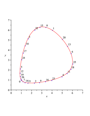
Figure 1: Oval of $\{V_{2,3}(x,y)=34\}$ with 27 iterates of $F_{2,3}$. The label $0$ indicates the initial condition $(1,1)$, and the label $k,k=1,\ldots,26,$ corresponds with the $k$-th point of the orbit.

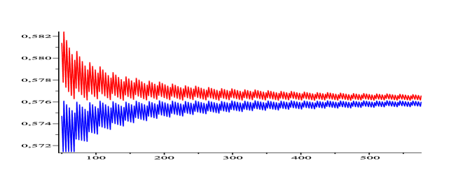
Figure 2: Lower and upper bounds for $\rho_{2,3}(34)$ obtained after following some points of the orbit starting at $(1,1)$.

We already know that the restriction of $F_{2,3}$ to the given oval is conjugated to a rotation, with rotation number $\rho:=\rho_{2,3}(34)$ that we want to estimate. This can be done by counting the number of turns that give the points $(x_{j},y_{j})$, after fixing some orientation in the closed curve. We orientate the curve with the counterclockwise sense. So, for instance we know that the second point $(x_{2},y_{2})$ has given more that one turn and less than two, giving that $1<2\rho<2,$ and hence that $\rho\in(1/2,1).$ Doing the same reasoning with all the points computed we obtain,

$$4<7\rho<5 \Rightarrow \rho\in\left(\frac{4}{7},\frac{5}{7}\right),$$

$$8<14\rho<9 \Rightarrow \rho\in\left(\frac{8}{14},\frac{9}{14}\right),$$

$$10<19\rho<11 \Rightarrow \rho\in\left(\frac{10}{19},\frac{11}{19}\right),$$

$$14<26\rho<15 \Rightarrow \rho\in\left(\frac{14}{26},\frac{15}{26}\right),$$

where we have only written the more relevant informacions obtained, which are given by the points of the orbit closer to the initial condition. So, we have shown that

$$0.5714\simeq\frac{4}{7}<\rho_{2,3}(34)<\frac{15}{26}\simeq 0.5769.$$

In Figure 2 we represent several successive lower and upper approximations obtained while the orbit is turning around the oval. We plot around six hundred steps, after skipping the first fifty ones. By taking 1000 points we get

$$0.5761246\simeq\frac{338}{578}<\rho_{2,3}(34)<\frac{473}{821}\simeq 0.5761267,$$

and after 3000 points,

$$0.57612457\simeq\frac{338}{578}<\rho_{2,3}(34)<\frac{1472}{2555}\simeq 0.57612524.$$

In fact when we say that $\rho_{2,3}(34)\in(\rho_{\mathrm{low}},\rho_{\mathrm{upp}})$, the value $\rho_{\mathrm{low}}$ is the upper lower bound obtained by following all the considered points of the orbit, and $\rho_{\mathrm{upp}}$ is the lowest upper bound. Notice that taking 1000 or 3000 points we have obtained the same lower bound for $\rho_{2,3}(34).$

Let us prove Theorem 3 by using the above approach.

Proof of Theorem 3. Consider $a=1/2,$ $b=3/2$ and the three points

$$\mathbf{p}^{1}=\left(\displaystyle{\frac{149}{100}},\displaystyle{\frac{173}{100}}\right),\quad\mathbf{p}^{2}=\left(\displaystyle{\frac{3}{40}},\displaystyle{\frac{173}{100}}\right),\quad\mathbf{p}^{3}=\left(\displaystyle{\frac{1}{1000}},\displaystyle{\frac{173}{100}}\right).$$

Notice that

$$h_{1}:=V_{3/2,1/2}(\mathbf{p}^{1})=\frac{10655559}{1288850}\simeq 8.27,$$

$$h_{2}:=V_{3/2,1/2}(\mathbf{p}^{2})=\frac{9328327}{207600}\simeq 44.93,$$

$$h_{3}:=V_{3/2,1/2}(\mathbf{p}^{3})=\frac{1056238343}{346000}\simeq 3052.71.$$

Hence $h_{c}<h_{1}<h_{2}<h_{3}.$ By applying the algorithm described above, using 100 points of each orbit starting at each ${\bf p}^{j},j=1,2,3,$ we obtain that

$$\rho_{3/2,1/2}(h_{1}),\rho_{3/2,1/2}(h_{3})\in\left(\frac{3}{5},\frac{59}{98}\right)\quad\mbox{and}\quad\rho_{3/2,1/2}(h_{2})\in\left(\frac{56}{93},\frac{53}{88}\right).$$

Since $59/98<56/93$ we have proved that the function $\rho_{3/2,1/2}(h)$ has at least a local maximum in $(h_{1},h_{3}).$ From the continuity of the rotation number function, with respect $a,b$ and $h$, we notice that this result also holds for all values of $a$ and $b$ in a neighborhood of $a=1/2,b=3/2.$    

We believe that with the same method it can be proved that a similar result to the one given in Theorem 3 holds for some maps $F_{c,b,a},$ but we have decided do not perform this study.

5.1 Some numerical explorations for $k=2.$

We start by studying with more detail the rotation number function $\rho_{3/2,1/2}(h)$, that we have considered to prove Theorem 3. In this case the fixed point is ${\bf p}\simeq(1.493363282,1.730133891)$ and $h_{c}=V_{b,a}({\mathbf{p}})=8.267483381.$ Moreover $\rho_{b,a}({h}_{c})\simeq 0.6006847931$. By applying our algorithm for approximating the rotation number, with $5000$ points on each orbit, we obtain the results presented in Table 1. In Figure 3 we also plot the upper and lower bounds of $\rho_{3/2,1/2}(h)$ that we have obtained by using a wide range of values of $h.$

Init. cond. $(x,\bar{y})$	Energy level $h$	$\rho_{\mathrm{low}}(h)\qquad$	$\rho_{\mathrm{upp}}(h)\qquad$
$\bar{x}$	$h_{c}\simeq 8.2675$	$\simeq 0.6006848$	$\simeq 0.6006848$
1.3	$8.3068$	$\frac{173}{288}\simeq 0.6006944$	$\frac{2938}{4891}\simeq 0.6006951$
0.75	$9.2747$	$\frac{1435}{2388}\simeq 0.6009213$	$\frac{2087}{3473}\simeq 0.6009214$
0.3	$14.7566$	$\frac{1548}{2573}\simeq 0.6016323$	$\frac{2285}{3798}\simeq 0.6016324$
0.075	$44.9347$	$\frac{657}{1091}\simeq 0.6021998$	$\frac{2354}{3909}\simeq 0.6022001$
0.001	$3052.75$	$\frac{2927}{4867}\simeq 0.6013972$	$\frac{86}{143}\simeq 0.6013986$
$5\cdot 10^{-6}$	$609716.07$	$\frac{1832}{3049}\simeq 0.6008527$	$\frac{1409}{2345}\simeq 0.6008529$
$5\cdot 10^{-256}$	$6.097\cdot 10^{255}$	$\frac{3}{5}=0.6$	$\frac{2999}{4998}\simeq 0.6000400$

Table 1: Lower and upper bounds of the rotation number $\rho_{3/2,1/2}(h)$, for some orbits of $F_{3/2,1/2}$ starting at $(x,\bar{y}),$ where ${\bf p}=(\bar{x},\bar{y}).$

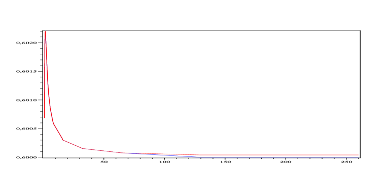
Figure 3: Lower and upper bounds for $\rho_{3/2,1/2}(h)$. On the horizontal axis we represent $-\log_{10}(h)$ and, on the vertical axis, the value of the rotation number. Notice that for values of $-\log_{10}(h)$ smaller that 70 both values are indistinguishable in the Figure.

For other values of $a$ and $b$ we obtain different behaviors. All the experiments are performed by starting at the fixed point ${\bf p}=(\bar{x},\bar{y}),$ and increasing the energy level by taking initial conditions of the form $(x,\overline{y})$, by decreasing $x$ to $0$. With this process we take orbits approaching to the boundary of ${Q^{+}}$, that is lying on level sets of $V_{b,a}$ with increasing energy. The step in the decrease of $x$ (and therefore in the increase of $h$) is not uniform, and it has been manually tuned making it smaller in those regions where a possible non monotonous behavior could appear.

Consider the set of parameters $\Gamma=\{(a,b),\in[0,\infty)^{2}\}$, where notice that we also consider the boundaries $a=0$ or $b=0,$ where the map $F_{b,a}$ is well defined. We already know that the rotation number function behaves equal at $(a,b)$ and $(b,a).$ Moreover we know perfectly its behavior on the diagonal $(a,a)$ (when $a<1$ it is monotonous decreasing and when $a>1$ it is monotonous increasing) and that $\rho_{1,1}(h)\equiv 4/5$ and $\rho_{0,0}(h)\equiv 2/3.$ Hence a good strategy for an numerical exploration can be to produce sequences of experiments using our algorithm by fixing some $a\geq 0$ and varying $b$. For instance we obtain:

• Case $a=1/2.$ For all the values of $b>0$ considered, the rotation number function seems to tend to $3/5$ when $h$ goes to infinity. Moreover it seems

  • monotone decreasing for $b\in\{1/4,1\};$

  • to have a unique maximum when $b\in\{7/5,3/2\}$;

  • monotone increasing for $b\in\{2,3\}.$

• Case $a=0.$ For all the values of $b>0$ considered, the rotation number function seems to tend to $5/8$ when $h$ goes to infinity. Moreover it seems

  • monotone decreasing for $b\in\{1/10,3/10,1/2\}$;

  • to have a unique maximum when $b\in\{7/10,3/4\}$;

  • monotone decreasing for $b\in\{1,5\}$.

The above results, together with some other experiments for other values of $a$ and $b$, not detailed in this paper, indicate the existence of a subset of positive measure in $\Gamma$ where the corresponding rotation number functions seem to present an unique maximum. This subset probably separates two other subsets of $\Gamma$, one where $\rho_{b,a}(h)$ is monotonically decreasing to $3/5$ , and another one where $\rho_{b,a}(h)$ increases monotonically to the same value. The “oscillatory subset” seems to shrink to $(a,b)=(1,1)$ when it approaches to the line $a=b$ and seems to finish in one interval on each of the borders $\{a=0\}$ and $\{b=0\}$. Further analysis must be done in this direction in order to have a more accurate knowledge of the bifurcation diagram associated to the behavior of $\rho_{b,a}$ on $\Gamma$.

References

- [1] W.J. Beyn, T. Hüls, M.Ch. Samtenschnieder. On –periodic orbits of –periodic maps, J. Difference Equ. Appl. 14 (2008), 865–887.
- [2] G. Bastien, M. Rogalski. Global behavior of the solutions of Lyness’ difference equation , J. Difference Equ. Appl. 10 (2004), 977–1003.
- [3] F. Beukers, R. Cushman. Zeeman’s monotonicity conjecture, J. Differential Equations 143 (1998), 191–200.
- [4] E. Camouzis, G. Ladas. Dynamics of third-order rational difference equations with open problems and conjectures. Advances in discrete mathematics and applications vol. 5. Chapman & Hall
- [5] A. Cima, A. Gasull, V. Maosa. Dynamics of the third order Lyness’ difference Equation, J. Difference Equ. Appl. 13 (2007), 855-884.
- [6] A. Cima, A. Gasull and V. Mañosa. Studying discrete dynamical systems through differential equations, J. Differential Equations 244 (2008), 630–648.
- [7] A. Cima, A. Gasull and V. Mañosa. On -periodic Lyness difference equations. In preparation 2010.
- [8] C.A. Clark, E.J. Janowski, M.R.S. Kulenović. Stability of the Gumowski–Mira equation with period–two coefficient, Int. J. Bifurcations & Chaos 17 (2007), 143–152.
- [9] V. de Angelis. Notes on the non–autonomous Lyness equation, J. Math. Anal and Appl. 307, 292–304 (2005).
- [10] S. Elaydi, R.J. Sacker. Global stability of periodic orbits of non–autonomous difference equations and population biology, J. Differential Equations 208, 258–273 (2005).
- [11] S. Elaydi, R.J. Sacker. Periodic difference equations, population biology and Cushing–Henson conjectures, Math. Biosciences 201, 195–207 (2006).
- [12] E.J. Janowski, M.R.S. Kulenović, Z. Nurkanović. Stability of the th order Lyness’ equation with period– coefficient, Int. J. Bifurcations & Chaos 17, 143–152 (2007).
- [13] D. Jogia, J. A. G. Roberts, F. Vivaldi, An algebraic geometric approach to integrable maps of the plane, J. Phys. A 39, 1133–1149 (2006).
- [14] M.R.S. Kulenović, Z. Nurkanović. Stability of Lyness’ equation with period–three coefficient, Radovi Matematički 12, 153–161 (2004).
- [15] J. Esch and T. D. Rogers, The screensaver map: dynamics on elliptic curves arising from polygonal folding, Discrete Comput. Geom. 25 (2001), 477–502 (2001).
- [16] J. Feuer, E.J. Janowski, G. Ladas. Invariants for some rational recursive sequaence with periodic coefficients, J. Difference Equations and Appl. 2, 167–174 (1996).
- [17] E.A. Grove, C.M. Kent and G. Ladas. Boundedness and persistence of nonautonomous Lyness and Max equations, J. Difference Equations and Appl. 3, 241–258 (1998).
- [18] E. C. Zeeman. Geometric unfolding of a difference equation, Hertford College, Oxford (1996). Unpublished.