Radius dependent shift of surface plasmon frequency in large metallic nanospheres: theory and experiment

Abstract

Theoretical description of oscillations of electron liquid in large metallic nanospheres (with radius of few tens nm) is formulated within random-phase-approximation semiclassical scheme. Spectrum of plasmons is determined including both surface and volume type excitations. It is demonstrated that only surface plasmons of dipole type can be excited by homogeneous dynamical electric field. The Lorentz friction due to irradiation of electro-magnetic wave by plasmon oscillations is analyzed with respect to the sphere dimension. The resulting shift of resonance frequency turns out to be strongly sensitive to the sphere radius. The form of e-m response of the system of metallic nanospheres embedded in the dielectric medium is found. The theoretical predictions are verified by a measurement of extinction of light due to plasmon excitations in nanosphere colloidal water solutions, for Au and Ag metallic components with radius from 10 to 75 nm. Theoretical predictions and experiments clearly agree in the positions of surface plasmon resonances and in an emergence of the first volume plasmon resonance in the e-m response of the system for limiting big nanosphere radii, when dipole approximation is not exact.

PACS No: 73.21.-b, 36.40.Gk, 73.20.Mf, 78.67.Bf

I Introduction

Experimental and theoretical investigations of plasmon excitations in metallic nanocrystals have received recently much attention due to possible applications in photo-voltaics and microelectronics. A significant enhancement of absorption of the incident light in photodiode-systems with active surface covered with metallic particles (of Au, Ag or Cu), with radius ten to several tens nanometers and with planar density $\sim 10^{8}$/cm², was observedwzmocn1 ; wzmocn2 ; wzr1 ; wzr2 ; wzr3 ; wzr4 ; wzr5 . This is due to mediating of light energy transfer by surface plasmon oscillations in metallic nano-components. These findings are of practical importance towards enhancement of solar cell efficiency especially for thin film cell technology. On the other side, hybridized states of surface plasmons and photons result in plasmon-polaritonsmaradudin which are of high significance for applications in sub-diffractional photonics and microelectronicszastos ; plasmons

For finite size crystals where the surface strongly affects the plasmon spectrum, surface plasmons occur and dominate the electro-magnetic (e-m) response of the metallic system. A strong dependence of resonance surface plasmon frequencies on the nanoparticle size and shape are reported in the literaturewzr2 ; burda . The plasmon resonances of noble metals, such as gold and silver (including also copper), are of particular interest due to their frequencies located within the visible part of the e-m spectrum.

Plasmon oscillations in metallic nanospheres can be excited by time-dependent electric field signal. There are different types of plasmon oscillations in the case of metallic nanoparticle. General types are volume and surface plasmons, referring to oscillations of internal electron density and surface electron density, respectively. The surface plasmons are linked to translational motion of all electrons which results in surface density oscillations only. The volume modes are related to compressional oscillations. Note that separation of these both types of collective excitations of electrons in metallic nanocrystal repeats the similar distinguishing of collective modes in atomic nucleimigdal ; steinw ; goldb (confirmed by giant resonance experiments). For metallic ultra-small clusters with number $N$ of electrons (in the range form $N=8$ to $N=200$ in Na clusters)brack the decoupling of volume and surface excitations is demonstrated by microscopic modelingbrack at approximately $N=50$. For ultra-small metallic clusters quantum shell effectsbrack and spill-out of electron cloud beyond the ionic jelliumekardt ; weick disturb separate formation of surface and volume collective excitations, while for large clusters (with radius larger than 10 nm) the role of shells and spill-out is considerably reducedbrack ; ekardt ; kresin , and both modes are well defined.

In order to excite the volume type oscillations an electric dynamical field inhomogeneous on the nanosphere scale is necessary while a homogeneous field excites only surface plasmons. For spherical symmetry, all modes of plasmon oscillations can be represented by spherical harmonics in terms of $l,m$, angular momentum (multiplicity) numbers. A dynamical electric field homogeneous over the sphere can induce only $l=1$, i.e., dipole-type surface oscillations.

The surface plasmons have been originally considered by Miemie , who provided a classical description of oscillations of electrical charge on the surface of the metallic sphere within the classical model. The dipole-type Mie oscillation energy is not dependent of the sphere radius, in contradiction to experimental observations, both in the case of small and larger nanospheres. For low radius, of order of single nanometers, besides mentioned above spill-out, the electron-electron interactions are importantburda ; brack ; ekardt ; kresin (including decay of plasmons into particle-hole pairs with similar energy, called as Landau dampingweick ; weick1 )—these quantum effects influence on position of resonance frequency. For large spheres, with radius bigger than 10 nm, even stronger shifts of resonance are observed, probably connected with another mechanism, since with radius growth quantum effects turn out to be not so important as for ultra-small clusters. The case of bigger nanospheres is, however, of particular significance as such metallic nano-components would be applied to enhancement of photo-voltaic effect in metallically modified solar cellswzmocn1 ; wzmocn2 ; wzr1 ; wzr2 ; wzr3 ; wzr4 .

Plasma excitations in metallic clusters were analyzed within many attitudes, addressed, however, mostly to small clusters. In particular were developed numerical methods of calculus ’ab initio’ including Kohn-Sham ’local density approximation [LDA], similar as applied in chemistry for large molecule calculations (limited, however, to few hundreds of electrons)serra ; ekardt ; brack . Also variational methods for energy density, semiclassical approachkresin and random-phase-approximation (RPA) numerical summations were applied (e.g., for clusters of Na with radius $\sim 1$nm)brack1 . Emerging of the Mie response from the more general description was analyzed, but including only (in a numerical manner) single breathing volume modebrack1 . Commonly the ’jellium’ model was applied, allowing for adiabatic approach to background ion system. In the ’jellium’ model all the kinetics concerns electron liquid screened by uniform and static background of positive ionsbrack ; ekart ; ksi .

Below we present the simplified RPA-type theory of plasmon excitations in metallic nanosphere embedded in dielectric medium adjusted to large nanospheres (with radius above 10 nm), when quantum corrections beyond semiclassical approximation are not so significant as in the case of ultra-small clustersbrack ; ekardt ; kresin . For optically induced plasma oscillations, the wavelength of incident light which excites resonance oscillations in metallic nanospheres (Au and Ag within several to several tens nm for radius) is considerably longer ($\lambda\sim 400$ nm) than nanosphere dimension. Thus, the dipole-type approximation is valid, i.e., one can assume that the electric field of the incident e-m wave is homogeneous over the nanosphere. Therefore, only dipole type oscillations of surface plasmons will contribute the resonance (except for limiting big nanospheres, when also volume excitations seem to enter e-m response due to not exact dipole approximation).

The experimentally observed red-shift of dipole Mie plasmon resonance for ultra-small clusters is caused mainly by significant spill-out effect reducing density of electronsbrack ; ekardt ; weick ; kresin . The Mie frequency is proportional to square root of the electron density and thus one arrives with reduced its value due to spill-out beyond the edge of ion jellium. With growing radius this effect weakens, as being of surface type and thus proportional to inverse radius, quite oppositely as red-shift observed for bigger nanospheres. For the radius over 10 nm the red-shift experimentally observed is much stronger than that one for small clusters and is sharply growing with radius enhancement. In order to explain this phenomenon observedwzr2 in nanospheres of Au and confirmed by more precise measurements for Au and Ag nanospheres reported in the present paper, we have included damping of plasmon oscillations via irradiation effects, which seem to dominate plasmon energy losses at larger scale of radii and cause strong red-shift of the resonance. We performed measurements of light extinction by nanospheres (in water colloidal solution) of Au with radii from 10 nm to 75 nm and Ag from 10 nm to 40 nm. The resulting data reveal a strong shift of resonance towards higher wave-lengths with radius growth. Radiation losses, which, as we suppose, are responsible for radius dependent red-shift of resonance frequency, can be described in terms of Lorentz frictionlan , and calculated also independently in Poyting vector terms in a far-field zone of plasmon radiation. Damping of plasmons is caused also additionally by electron scattering processes and we verify that this channel is not important for $a>20$ nm ($a$—nanosphere radius) when radiation losses are much stronger. The shift of the resonance frequency of dipole-type surface plasmons resulting due to damping phenomena is compared with the experimental data for various nanosphere radii. Emerging of the first mode of volume plasmons is experimentally observed for $2a\sim 150$ nm for Au and $2a\sim 80$ nm for Ag, due to breaking the dipole approximation at this range of radius, in agreement with the presented theory predictions.

The paper is organized as follows. In the first paragraph, the RPA theoryrpa ; pines ; jac is generalized for the confined system of spherical shape. In the second one, the equations for volume and surface plasmons are solved (with particularities of calculus in the Appendix). The third paragraph contains a description of the Lorentz friction for surface plasmons oscillations of the dipole-type. In the fourth one, an analysis of the radiation losses is presented using the Poyting vector of plasmon radiation in far-field region, which supports the previous Lorentz friction estimation. The following paragraph comprises the summarizing of whole e-m response of metallic nanosphere system. The last paragraph presents a comparison of the theoretical predictions with experimental data of e-m response features of the colloidal water solutions with nanospheres of Au and Ag with several radii of metallic nano-components.

II RPA semiclassical approach to electron excitations in metallic nanosphere

II.1 Derivation of RPA equation for local electron density in spherical geometry

Let us consider a metallic sphere with a radius $a$, located for the starting model in the vacuum, $\varepsilon=1,\;\mu=1$ and in the presence of a dynamical electric field (magnetic field is assumed zero). The model jelliumbrack ; ekart ; ksi is assumed in order to account for the screening background of positive ions in the form of static uniformly distributed over the sphere positive charge:

$$n_{e}({\bm{r}})=n_{e}\Theta(a-r),$$ (1)

where $n_{e}=N_{e}/V$ with $n_{e}|e|$ is the averaged positive charge density, $N_{e}$ is the number of collective electrons in the sphere, $V=\frac{4\pi a^{3}}{3}$ is the sphere volume, and $\Theta$ is the Heaviside step-function. After neglecting the ion dynamics within the jellium model, which can be adopted in particular for description of simple metals, as noble, transition and alkali metals, we deal with the Hamiltonian for collective electrons,

$$\hat{H}_{e}=\sum\limits_{j=1}^{N_{e}}\left[-\frac{\hbar^{2}\nabla_{j}^{2}}{2m}-e^{2}\int\frac{n_{e}({\bm{r}_{0}})d^{3}{\bm{r}_{0}}}{|{\bm{r}}_{j}-{\bm{r}_{0}}|}+e\varphi({\bm{r}}_{j},t)\right]+\frac{1}{2}\sum\limits_{j\neq j^{\prime}}\frac{e^{2}}{|{\bm{r}}_{j}-{\bm{r}}_{j^{\prime}}|}+\Delta E,$$ (2)

where ${\bm{r}}_{j}$ and $m$ are the position (with respect to the dot center) and mass of $j$th electron, $\Delta E$ represents the electrostatic energy contribution from the ion jellium, and $\varphi({\bm{r}},t)$ is the scalar potential of the external electric field. The corresponding electric field ${\bm{E}}({\bm{r}}_{j},t)=-\nabla\varphi({\bm{r}}_{j},t)$. Assuming that space-dependence of ${\bm{E}}$ is weak on the scale of the sphere radius $a$ (i.e the electric field is homogeneous over the sphere), $\varphi({\bm{r}}_{j},t)=-{\bm{r}}_{j}\cdot\bm{E}(t)$.

A local electron density can be written as followsrpa :

$$\rho({\bm{r}},t)=<\Psi({\bm{r}_{e}},t)|\sum\limits_{j}\delta({\bm{r}}-{\bm{r}}_{j})|\Psi({\bm{r}_{e}},t)>,$$ (3)

$i\hbar\frac{\partial\Psi({\bm{r}_{e}},t)}{\partial t}=\hat{H}_{e}\Psi({\bm{r}_{e}},t)$, ${\bm{r}_{e}}=({\bm{r}_{1}},{\bm{r}_{2}},...,{\bm{r}_{N}})$, with the Fourier picture:

$$\tilde{\rho}({\bm{k}},t)=\int\rho({\bm{r}},t)e^{-i{\bm{k}}\cdot{\bm{r}}}d^{3}r=<\Psi^{\prime}({\bm{r}_{e}},t)|\hat{\rho}({\bm{k}})|\Psi^{\prime}({\bm{r}_{e}},t)>,$$ (4)

where the ’operator’ $\hat{\rho}({\bm{k}})=\sum\limits_{j}e^{-i{\bm{k}}\cdot{\bm{r}_{j}}}$.

Using the above notation one can rewrite $\hat{H}_{e}$, in analogy to the bulk casepines , in the following form:

$$\begin{array}[]{l}\hat{H}_{e}=\sum\limits_{j=1}^{N_{e}}\left[-\frac{\hbar^{2}\nabla_{j}^{2}}{2m}\right]-\frac{e^{2}}{4\pi^{2}}\int d^{3}k\tilde{n}_{e}({\bm{k}})\frac{1}{k^{2}}\left(\hat{\rho^{+}}({\bm{k}})+\hat{\rho}({\bm{k}})\right)\\ +\frac{e^{2}}{16\pi^{3}}\int d^{3}k\tilde{\varphi}({\bm{k}},t)\left(\hat{\rho^{+}}({\bm{k}})+\hat{\rho}({\bm{k}})\right)+\frac{e^{2}}{4\pi^{2}}\int d^{3}k\frac{1}{k^{2}}\left[\hat{\rho^{+}}({\bm{k}})\hat{\rho}({\bm{k}})-N_{e}\right]+\Delta E,\\ \end{array}$$ (5)

where: $\tilde{n}_{e}({\bm{k}})=\int d^{3}rn_{e}({\bm{r}})e^{-i{\bm{k}}\cdot{\bm{r}}}$, $\frac{4\pi}{k^{2}}=\int d^{3}r\frac{1}{r}e^{-i{\bm{k}}\cdot{\bm{r}}}$, $\tilde{\varphi}({\bm{k}})=\int d^{3}r\varphi({\bm{r}},t)e^{-i{\bm{k}}\cdot{\bm{r}}}$.

Utilizing this form of the electron Hamiltonian one can write the motion equation for $\hat{\rho}({\bm{k}})$:

$$\frac{d^{2}\hat{\rho}({\bm{k}})}{dt^{2}}=\frac{1}{(i\hbar)^{2}}\left[\left[\hat{\rho}({\bm{k}}),\hat{H}_{e}\right],\hat{H}_{e}\right],$$ (6)

or, after some algebra:

$$\begin{array}[]{l}\frac{d^{2}\delta\hat{\rho}({\bm{k}})}{dt^{2}}=-\sum\limits_{j}e^{-i{\bm{k}}\cdot{\bm{r}}_{j}}\left\{-\frac{\hbar^{2}}{m^{2}}\left({\bm{k}}\cdot\nabla_{j}\right)^{2}+\frac{\hbar^{2}k^{2}}{m^{2}}i{\bm{k}}\cdot\nabla_{j}+\frac{\hbar^{2}k^{4}}{4m^{2}}\right\}\\ -\frac{e^{2}}{m2\pi^{2}}\int d^{3}q\tilde{n}_{e}({\bm{k}}-{\bm{q}})\frac{{\bm{k}}\cdot{\bm{q}}}{q^{2}}\delta\hat{\rho}({\bm{q}})-\frac{e}{m8\pi^{3}}\int d^{3}q\tilde{n}_{e}({\bm{k}}-{\bm{q}})({\bm{k}}\cdot{\bm{q}})\tilde{\varphi}({\bm{q}},t)\\ -\frac{e}{m8\pi^{3}}\int d^{3}q\delta\hat{\rho}({\bm{k}}-{\bm{q}})({\bm{k}}\cdot{\bm{q}})\tilde{\varphi}({\bm{q}},t)-\frac{e^{2}}{m2\pi^{2}}\int d^{3}q\delta\hat{\rho}({\bm{k}}-{\bm{q}})\frac{{\bm{k}}\cdot{\bm{q}}}{q^{2}}\delta\hat{\rho}({\bm{q}}),\\ \end{array}$$ (7)

where $\delta\hat{\rho}({\bm{k}})=\hat{\rho}({\bm{k})}-\tilde{n}_{e}({\bm{k}})$ is the ’operator’ of local electron density fluctuations beyond the uniform distribution. Taking into account that: $\delta\tilde{\rho}({\bm{k}},t)=<\Psi(t)|\delta\hat{\rho}({\bm{k}})|\Psi(t)>=\tilde{\rho}({\bm{k}},t)-\tilde{n}_{e}({\bm{k}})$ we find:

$$\begin{array}[]{l}\frac{\partial^{2}\delta\tilde{\rho}({\bm{k}},t)}{\partial t^{2}}=<\Psi|-\sum\limits_{j}e^{-i{\bm{k}}\cdot{\bm{r}}_{j}}\left\{-\frac{\hbar^{2}}{m^{2}}\left({\bm{k}}\cdot\nabla_{j}\right)^{2}+\frac{\hbar^{2}k^{2}}{m^{2}}i{\bm{k}}\cdot\nabla_{j}+\frac{\hbar^{2}k^{4}}{4m^{2}}\right\}|\Psi>\\ -\frac{e^{2}}{m2\pi^{2}}\int d^{3}q\tilde{n}_{e}({\bm{k}}-{\bm{q}})\frac{{\bm{k}}\cdot{\bm{q}}}{q^{2}}\delta\tilde{\rho}({\bm{q}},t)-\frac{e}{m8\pi^{3}}\int d^{3}q\tilde{n}_{e}({\bm{k}}-{\bm{q}})({\bm{k}}\cdot{\bm{q}})\tilde{\varphi}({\bm{q}},t)\\ -\frac{e}{m8\pi^{3}}\int d^{3}q\delta\tilde{\rho}({\bm{k}}-{\bm{q}},t)({\bm{k}}\cdot{\bm{q}})\tilde{\varphi}({\bm{q}},t)-\frac{e^{2}}{m2\pi^{2}}\int d^{3}q\frac{{\bm{k}}\cdot{\bm{q}}}{q^{2}}<\Psi|\delta\hat{\rho}({\bm{k}}-{\bm{q}})\delta\hat{\rho}({\bm{q}})|\Psi>,\\ \end{array}$$ (8)

One can simplify the above equation using the assumption that $\delta\rho({\bm{r},t})=\frac{1}{8\pi^{3}}\int e^{i{\bm{k}}\cdot{\bm{r}}}\delta\tilde{\rho}({\bm{k}},t)d^{3}k$ only weakly varies on the interatomic scale, and hence three components of the first term in right-hand-side of Eq. (8) can be estimated as: $k^{2}v_{F}^{2}\delta\tilde{\rho}({\bm{k}},t)$, $k^{3}v_{F}/k_{T}\delta\tilde{\rho}({\bm{k}},t)$ and $k^{4}v_{F}^{2}/k_{T}^{2}\delta\tilde{\rho}({\bm{k}},t)$, respectively ($1/k_{T}$ is Thomas-Fermi radiusrpa , $k_{T}=\sqrt{\frac{6\pi n_{e}e^{2}}{\epsilon_{F}}}$, $\epsilon_{F}$—the Fermi energy, $v_{F}$—the Fermi velocity). Thus the contribution of the second and the third components of the first term can be neglected in comparison to the first component. Small and thus negligible is also the last term in right-hand-side of Eq. (8), as it involves a product of two $\delta\tilde{\rho}$ (which we assumed small $\delta\tilde{\rho}/n_{e}<<1$). This approach corresponds to random-phase-approximation (RPA) attitude formulated for bulk metalrpa ; pines (note that $\delta\hat{\rho}(0)=0$ and the coherent RPA contribution of interaction is contained in the second term in the right-hand-side of Eq. (8)). The last but one term in Eq. (8)) can be reduced if to confine only to linear terms with respect to $\delta\tilde{\rho}$ and $\tilde{\varphi}$. Next, due to spherical symmetry, $<\Psi|\sum\limits_{j}e^{-i{\bm{k}}\cdot{\bm{r}}_{j}}\frac{\hbar^{2}}{m^{2}}\left({\bm{k}}\cdot\nabla_{j}\right)^{2}|\Psi>\simeq\frac{2k^{2}}{3m}<\Psi|\sum\limits_{j}e^{-i{\bm{k}}\cdot{\bm{r}}_{j}}\frac{\hbar^{2}\nabla_{j}^{2}}{2m}|\Psi>$. After the inverse Fourier transform, Eq. (8) attains the form:

$$\begin{array}[]{l}\frac{\partial^{2}\delta\rho({\bm{r}},t)}{\partial t^{2}}=-\frac{2}{3m}\nabla^{2}<\Psi|\sum\limits_{j}\delta({\bm{r}}-{\bm{r}}_{j})\frac{\hbar^{2}\nabla_{j}^{2}}{2m}|\Psi>\\ +\frac{\omega_{p}^{2}}{4\pi}\nabla\left\{\Theta(a-r)\nabla\int d^{3}r_{1}\frac{1}{|{\bm{r}}-{\bm{r}}_{1}|}\delta\rho({\bm{r}}_{1},t)\right\}+\frac{en_{e}}{m}\nabla\left\{\Theta(a-r)\nabla\varphi({\bm{r}},t)\right\}.\\ \end{array}$$ (9)

According to Thomas-Fermi approximationrpa the averaged kinetic energy can be represented as follows:

$$\begin{array}[]{l}<\Psi|-\sum\limits_{j}\delta({\bm{r}}-{\bm{r}}_{j})\frac{\hbar^{2}\nabla_{j}^{2}}{2m}|\Psi>\simeq\frac{3}{5}(3\pi^{2})^{2/3}\frac{\hbar^{2}}{2m}\rho^{5/3}({\bm{r}})\\ =\frac{3}{5}(3\pi^{2})^{2/3}\frac{\hbar^{2}}{2m}n_{e}^{5/3}\Theta(a-r)\left[1+\frac{5}{3}\frac{\delta\rho({\bm{r}})}{n_{e}}+...\right].\\ \end{array}$$ (10)

Taking into account the above approximation and that $\nabla\Theta(a-r)=-\frac{\bm{r}}{r}\delta(a-r)=-\frac{\bm{r}}{r}\lim_{\epsilon\rightarrow 0}\delta(a+\epsilon-r)$ as well as that $\varphi({\bm{r}},t)=-{\bm{r}}\cdot{\bm{E}}(t)$, one can rewrite Eq. (9) in the following manner:

$$\begin{array}[]{l}\frac{\partial^{2}\delta\rho({\bm{r}},t)}{\partial t^{2}}=\left[\frac{2}{3}\frac{\epsilon_{F}}{m}\nabla^{2}\delta\rho({\bm{r}},t)-\omega_{p}^{2}\delta\rho({\bm{r}},t)\right]\Theta(a-r)\\ -\frac{2}{3m}\nabla\left\{\left[\frac{3}{5}\epsilon_{F}n_{e}+\epsilon_{F}\delta\rho({\bm{r}},t)\right]\frac{\bm{r}}{r}\delta(a+\epsilon-r)\right\}\\ -\left[\frac{2}{3}\frac{\epsilon_{F}}{m}\frac{\bm{r}}{r}\nabla\delta\rho({\bm{r}},t)+\frac{\omega_{p}^{2}}{4\pi}\frac{\bm{r}}{r}\nabla\int d^{3}r_{1}\frac{1}{|{\bm{r}}-{\bm{r}}_{1}|}\delta\rho({\bm{r}}_{1},t)+\frac{en_{e}}{m}\frac{\bm{r}}{r}\cdot{\bm{E}}(t)\right]\delta(a+\epsilon-r).\\ \end{array}$$ (11)

In the above formula $\omega_{p}$ is the bulk plasmon frequency, $\omega_{p}^{2}=\frac{4\pi n_{e}e^{2}}{m}$, and $\delta(a+\epsilon-r)=\lim_{\epsilon\rightarrow 0}\delta(a+\epsilon-r)$. The solution of Eq. (11) can be decomposed into two parts with regard to the domain:

$$\delta\rho({\bm{r},t})=\left\{\begin{array}[]{l}\delta\rho_{1}({\bm{r},t}),\;for\;r<a,\\ \delta\rho_{2}({\bm{r},t}),\;for\;r\geq a,\;(r\rightarrow a+),\\ \end{array}\right.$$ (12)

corresponding to the volume and surface excitations, respectively. These two parts of local electron density fluctuations satisfy the equations:

$$\frac{\partial^{2}\delta\rho_{1}({\bm{r}},t)}{\partial t^{2}}=\frac{2}{3}\frac{\epsilon_{F}}{m}\nabla^{2}\delta\rho_{1}({\bm{r}},t)-\omega_{p}^{2}\delta\rho_{1}({\bm{r}},t),$$ (13)

and

$$\begin{array}[]{l}\frac{\partial^{2}\delta\rho_{2}({\bm{r}},t)}{\partial t^{2}}=-\frac{2}{3m}\nabla\left\{\left[\frac{3}{5}\epsilon_{F}n_{e}+\epsilon_{F}\delta\rho_{2}({\bm{r}},t)\right]\frac{\bm{r}}{r}\delta(a+\epsilon-r)\right\}\\ -\left[\frac{2}{3}\frac{\epsilon_{F}}{m}\frac{\bm{r}}{r}\nabla\delta\rho_{2}({\bm{r}},t)+\frac{\omega_{p}^{2}}{4\pi}\frac{\bm{r}}{r}\nabla\int d^{3}r_{1}\frac{1}{|{\bm{r}}-{\bm{r}}_{1}|}\left(\delta\rho_{1}({\bm{r}}_{1},t)\Theta(a-r_{1})\right.\right.\\ \left.\left.+\delta\rho_{2}({\bm{r}}_{1},t)\Theta(r_{1}-a)\right)+\frac{en_{e}}{m}\frac{\bm{r}}{r}\cdot{\bm{E}}(t)\right]\delta(a+\epsilon-r).\\ \end{array}$$ (14)

It is clear from Eq. (13) that the volume plasmons are independent of surface plasmons. However, surface plasmons can be excited by volume plasmons due to the last term in Eq. (14) (corresponding to ’a surface tail’ of volume oscillations), which expresses a coupling between surface and volume oscillations in the metallic nanosphere within the above semiclassical RPA approach.

In a dielectric medium in which the metallic sphere can be embedded, the electrons on the surface interact with forces $\varepsilon$ (dielectric constant) times weaker in comparison to electrons inside the sphere. To account for it, one can substitute Eq. (14) with the following one (Eq. (13) does not change):

$$\begin{array}[]{l}\frac{\partial^{2}\delta\rho_{2}({\bm{r}},t)}{\partial t^{2}}=-\frac{2}{3m}\nabla\left\{\left[\frac{3}{5}\epsilon_{F}n_{e}+\epsilon_{F}\delta\rho_{2}({\bm{r}},t)\right]\frac{\bm{r}}{r}\delta(a+\epsilon-r)\right\}\\ -\left[\frac{2}{3}\frac{\epsilon_{F}}{m}\frac{\bm{r}}{r}\nabla\delta\rho_{2}({\bm{r}},t)+\frac{\omega_{p}^{2}}{4\pi}\frac{\bm{r}}{r}\nabla\int d^{3}r_{1}\frac{1}{|{\bm{r}}-{\bm{r}}_{1}|}\left(\delta\rho_{1}({\bm{r}}_{1},t)\Theta(a-r_{1})\right.\right.\\ \left.\left.+\frac{1}{\varepsilon}\delta\rho_{2}({\bm{r}}_{1},t)\Theta(r_{1}-a)\right)+\frac{en_{e}}{m}\frac{\bm{r}}{r}\cdot{\bm{E}}(t)\right]\delta(a+\epsilon-r).\\ \end{array}$$ (15)

Let us also assume that both volume and surface plasmon oscillations are damped with the time ratio $\tau_{0}$ which can be phenomenologically accounted for via the additional term, $-\frac{2}{\tau_{0}}\frac{\partial\delta\rho({\bm{r}},t)}{\partial t}$, to the right-hand-side of above equations. They attain the form:

$$\frac{\partial^{2}\delta\rho_{1}({\bm{r}},t)}{\partial t^{2}}+\frac{2}{\tau_{0}}\frac{\partial\delta\rho_{1}({\bm{r}},t)}{\partial t}=\frac{2}{3}\frac{\epsilon_{F}}{m}\nabla^{2}\delta\rho_{1}({\bm{r}},t)-\omega_{p}^{2}\delta\rho_{1}({\bm{r}},t),$$ (16)

and

$$\begin{array}[]{l}\frac{\partial^{2}\delta\rho_{2}({\bm{r}},t)}{\partial t^{2}}+\frac{2}{\tau_{0}}\frac{\partial\delta\rho_{2}({\bm{r}},t)}{\partial t}=-\frac{2}{3m}\nabla\left\{\left[\frac{3}{5}\epsilon_{F}n_{e}+\epsilon_{F}\delta\rho_{2}({\bm{r}},t)\right]\frac{\bm{r}}{r}\delta(a+\epsilon-r)\right\}\\ -\left[\frac{2}{3}\frac{\epsilon_{F}}{m}\frac{\bm{r}}{r}\nabla\delta\rho_{2}({\bm{r}},t)+\frac{\omega_{p}^{2}}{4\pi}\frac{\bm{r}}{r}\nabla\int d^{3}r_{1}\frac{1}{|{\bm{r}}-{\bm{r}}_{1}|}\left(\delta\rho_{1}({\bm{r}}_{1},t)\Theta(a-r_{1})\right.\right.\\ \left.\left.+\frac{1}{\varepsilon}\delta\rho_{2}({\bm{r}}_{1},t)\Theta(r_{1}-a)\right)+\frac{en_{e}}{m}\frac{\bm{r}}{r}\cdot{\bm{E}}(t)\right]\delta(a+\epsilon-r).\\ \end{array}$$ (17)

From Eqs (16) and (17) it is noticeable that the homogeneous electric field does not excite the volume-type plasmons but only induces the surface plasmons.

The derived above equations for plasmon excitations in spherical metallic system are in agreement with other similar semiclassical approximations reviewed e.g., in Ref. kresin, .

II.2 Solution of RPA equations: volume and surface plasmons frequencies

Eqs (16, 17) can be solved upon imposed the boundary and initial conditions (cf. Appendix A). Let us represent both parts of the electron fluctuation in the following manner:

$$\begin{array}[]{l}\delta\rho_{1}({\bm{r},t})=n_{e}\left[f_{1}(r)+F({\bm{r}},t)\right],\;for\;r<a,\\ \delta\rho_{2}({\bm{r},t})=n_{e}f_{2}(r)+\sigma(\Omega,t)\delta(r+\epsilon-a),\;for\;r\geq a,\;(r\rightarrow a+),\\ \end{array}$$ (18)

and let us choose the convenient initial conditions, $F({\bm{r}},t)|_{t=0}=0,\;\sigma(\Omega,t)|_{t=0}=0$, ($\Omega=(\theta,\psi)$—the spherical angles), moreover, $(1+f_{1}(r))|_{r=a}=f_{2}(r)|_{r=a}$ (continuity condition), $F({\bm{r}},t)|_{r=a}=0$, $\int\rho({\bm{r}},t)d^{3}r=N_{e}$ (neutrality condition).

We arrive thus with the explicit form of the solutions of Eqs (16) and (17) (cf. Appendix A):

$$\begin{array}[]{l}f_{1}(r)=-\frac{k_{T}a+1}{2}e^{-k_{T}(a-r)}\frac{1-e^{-2k_{T}r}}{k_{T}r},\;for\;\;r<a,\\ f_{2}(r)=\left[k_{T}a-\frac{k_{T}a+1}{2}\left(1-e^{-2k_{T}a}\right)\right]\frac{e^{-k_{T}(r-a)}}{k_{T}r},\;for\;\;r\geq a,\\ \end{array}$$ (19)

where $k_{T}=\sqrt{\frac{6\pi n_{e}e^{2}}{\epsilon_{F}}}=\sqrt{\frac{3\omega_{p}^{2}}{v_{F}^{2}}}$, and for time-dependent parts:

$$F({\bm{r}},t)=\sum\limits_{l=1}^{\infty}\sum\limits_{m=-l}^{l}\sum\limits_{n=1}^{\infty}A_{lmn}j_{l}(k_{nl}r)Y_{lm}(\Omega)sin(\omega^{\prime}_{nl}t)e^{-t/\tau_{0}},$$ (20)

and

$$\begin{array}[]{l}\sigma(\Omega,t)=\sum\limits_{l=1}^{\infty}\sum\limits_{m=-l}^{l}Y_{lm}(\Omega)\left[\frac{B_{lm}}{a^{2}}sin(\omega^{\prime}_{0l}t)e^{-t/\tau_{0}}(1-\delta_{1l})+Q_{1m}(t)\delta_{1l}\right]\\ +\sum\limits_{l=1}^{\infty}\sum\limits_{m=-l}^{l}\sum\limits_{n=1}^{\infty}A_{lmn}\frac{(l+1)\omega_{p}^{2}}{l\omega_{p}^{2}-(2l+1)\omega_{nl}^{2}}Y_{lm}(\Omega)n_{e}\int\limits_{0}^{a}dr_{1}\frac{r_{1}^{l+2}}{a^{l+2}}j_{l}(k_{nl}r_{1})sin(\omega^{\prime}_{nl}t)e^{-t/\tau_{0}},\\ \end{array}$$ (21)

where $j_{l}(\xi)=\sqrt{\frac{\pi}{2\xi}}I_{l+1/2}(\xi)$ is the spherical Bessel function, $Y_{lm}(\Omega)$ is the spherical function, $\omega_{nl}=\omega_{p}\sqrt{1+\frac{x_{nl}^{2}}{k_{T}^{2}a^{2}}}$ are the frequencies of electron volume free self-oscillations (volume plasmon frequencies), $x_{nl}$ are nodes of the Bessel function $j_{l}(\xi)$, $\omega_{0l}=\omega_{p}\sqrt{\frac{l}{2l+1}}$ are the frequencies of electron surface free self-oscillations (surface plasmon frequencies), and $k_{nl}=x_{nl}/a$; $\omega^{\prime}=\sqrt{\omega^{2}-\frac{1}{\tau_{0}^{2}}}$ are the shifted frequencies for all modes due to damping. The coefficients $B_{lm}$ and $A_{lmn}$ can be determined by the initial conditions. As we have assumed that $\delta\rho({\bm{r}},t=0)=0$, we get $B_{lm}=0$ and $A_{lmn}=0$, except for $l=1$ in the former case (of $B_{lm}$), corresponding to response to homogeneous electric field. This mode is described by the function $Q_{1m}(t)$ in the general solution (21). The function $Q_{1m}(t)$ satisfies the equation:

$$\begin{array}[]{l}\frac{\partial^{2}Q_{1m}(t)}{\partial t^{2}}+\frac{2}{\tau_{0}}\frac{\partial Q_{1m}(t)}{\partial t}+\omega_{1}^{2}Q_{1m}(t)\\ =\sqrt{\frac{4\pi}{3}}\frac{en_{e}}{m}\left[E_{z}(t)\delta_{m0}+\sqrt{2}\left(E_{x}(t)\delta_{m1}+E_{y}(t)\delta_{m-1}\right)\right],\\ \end{array}$$ (22)

where $\omega_{1}=\omega_{01}=\frac{\omega_{p}}{\sqrt{3\varepsilon}}$ (it is a dipole-type surface plasmon Mie frequencymie ). Only this function contributes the dynamical response to the homogeneous electric field (for the assumed initial conditions). From the above it follows thus that local electron density (within semiclassical RPA attitude) has the form:

$$\rho({\bm{r}},t)=\rho_{0}(r)+\rho_{1}({\bm{r}},t),$$ (23)

with the RPA equilibrium electron distribution (correcting the uniform distribution $n_{e}$):

$$\rho_{0}(r)=\left\{\begin{array}[]{l}n_{e}\left[1+f_{1}(r)\right],\;for\;\;r<a,\\ n_{e}f_{2}(r),\;for\;\;r\geq a,\;r\rightarrow a+\\ \end{array}\right.$$ (24)

and the nonequilibrium part, of surface plasmon oscillation type:

$$\rho_{1}({\bm{r}},t)=\left\{\begin{array}[]{l}0,\;for\;\;r<a,\\ \sum\limits_{m=-1}^{1}Q_{1m}(t)Y_{1m}(\Omega)\;for\;\;r\geq a,\;r\rightarrow a+.\\ \end{array}\right.$$ (25)

In general, $F({\bm{r}},t)$ (volume plasmons) and $\sigma(\Omega,t)$ (surface plasmons) contribute to plasmon e-m response. However, in the case of homogeneous perturbation, only the surface $l=1$ mode is excited.

For plasmon oscillations given by Eq. (25) one can calculate the corresponding dipole,

$${\bm{D}}(t)=e\int d^{3}r{\bm{r}}\rho({\bm{r}},t)=\frac{4\pi}{3}e{\bm{q}}(t)a^{3},$$ (26)

where $Q_{11}(t)=\sqrt{\frac{8\pi}{3}}q_{x}(t)$, $Q_{1-1}(t)=\sqrt{\frac{8\pi}{3}}q_{y}(t)$, $Q_{10}(t)=\sqrt{\frac{4\pi}{3}}q_{x}(t)$ and ${\bm{q}}(t)$ satisfies the equation (cf. Eq. (22)),

$$\left[\frac{\partial^{2}}{\partial t^{2}}+\frac{2}{\tau_{0}}\frac{\partial}{\partial t}+\omega_{1}^{2}\right]{\bm{q}}(t)=\frac{en_{e}}{m}{\bm{E}}(t).$$ (27)

III Lorentz friction for nanosphere plasmons

The nanosphere plasmons induced by a homogeneous electric field, as described in the above paragraph, are themselves a source of the e-m radiation. This radiation takes away the energy of plasmons resulting in their damping, which can be described as the Lorentz frictionlan . This damping was not included in $\tau_{0}$ in Eq. (22). The e-m wave emission which causes electron friction can be described as the additional electric fieldlan ,

$${\bm{E}}_{L}=\frac{2}{3\varepsilon v^{2}}\frac{\partial^{3}{\bm{D}}(t)}{\partial t^{3}},$$ (28)

where $v=\frac{c}{\sqrt{\varepsilon}}$ is the light velocity in the dielectric medium, and ${\bm{D}}(t)$ is the dipole of the nanosphere. According to Eq. (26) we arrive at the following relation,

$${\bm{E}}_{L}=\frac{2e}{3\varepsilon v^{2}}\frac{4\pi}{3}a^{3}\frac{\partial^{3}{\bm{q}}(t)}{\partial t^{3}}.$$ (29)

Substituting it into Eq. (27) we get

$$\left[\frac{\partial^{2}}{\partial t^{2}}+\frac{2}{\tau_{0}}\frac{\partial}{\partial t}+\omega_{1}^{2}\right]{\bm{q}}(t)=\frac{en_{e}}{m}{\bm{E}}(t)+\frac{2}{3\omega_{1}}\left(\frac{\omega_{1}a}{v}\right)^{3}\frac{\partial^{3}{\bm{q}}(t)}{\partial t^{3}}.$$ (30)

If one assumes the estimation $\frac{\partial^{3}{\bm{q}}(t)}{\partial t^{3}}\simeq-\omega_{1}^{2}\frac{\partial{\bm{q}}(t)}{\partial t}$ (resulting from perturbative method of solution of the above equation), then one can include the Lorentz friction in a renormalized damping term:

$$\left[\frac{\partial^{2}}{\partial t^{2}}+\frac{2}{\tau}\frac{\partial}{\partial t}+\omega_{1}^{2}\right]{\bm{q}}(t)=\frac{en_{e}}{m}{\bm{E}}(t),$$ (31)

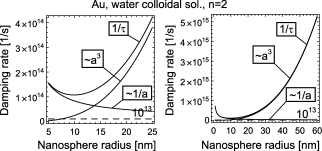
Figure 1: Damping rate $\frac{1}{\tau}$ of surface plasmons calculated according to the formula (32) versus nanosphere radius for Au (in water colloidal solution with refraction factor $n=2$ in Eq. (32) $C=2$, $\lambda_{B}=5.3\cdot 10^{-8}$ m), dashed line—$10^{13}$ 1/s level

where (cf. Fig. 1),

$$\frac{1}{\tau}=\frac{1}{\tau_{0}}+\frac{\omega_{1}}{3}\left(\frac{\omega_{1}a}{v}\right)^{3}\simeq\frac{v_{F}}{2\lambda_{B}}+\frac{Cv_{F}}{2a}+\frac{\omega_{1}}{3}\left(\frac{\omega_{1}a}{v}\right)^{3},$$ (32)

where we used for $\frac{1}{\tau_{0}}\simeq\frac{v_{F}}{2\lambda_{B}}+\frac{Cv_{F}}{2a}$ ($\lambda_{B}$ is the free path in bulk, $v_{F}$ the Fermi velocity, and $C\simeq 1$ is a constant)atwater ; kr which corresponds to inclusion of plasmon damping due to electron scattering on other electrons, on impurities, on phonons and on nanocrystal boundary. The renormalized damping causes the change in the shift of self-frequency of free surface plasmons, $\omega_{1}^{\prime}=\sqrt{\omega_{1}^{2}-\frac{1}{\tau^{2}}}$.

Using Eq. (32) one can determine the radius $a_{0}$ corresponding to a minimal damping,

$$a_{0}=\frac{\sqrt{3}}{\omega_{p}}\left(v_{F}c^{3}\sqrt{\varepsilon}/2\right)^{1/4}.$$ (33)

III.1 Radiation of surface plasmons on metallic nanosphere in far-field zone

The Lorentz friction mechanism of energy losses of dipole surface oscillations described above can be also analyzed equivalently by accounting for e-m emission from oscillating dipoles of plasmons. Let us consider Eq. (27) with irradiation induced damping included into $\tau$ (instead of $\tau_{0}$). For $E(t)=E_{0}[1-\Theta(t)]$ (the rapid switching off a constant electric field $E_{0}$) the solution of Eq. (27) has the form:

$$q(t)=\sqrt{\frac{4\pi}{3}}\frac{en_{e}}{m\omega_{1}^{2}}E_{0}\left\{\begin{array}[]{l}1,\;\;for\;\;t<0,\\ \left[cos(\omega_{1}t)+\frac{sin(\omega_{1}t)}{\omega_{1}\tau}\right]e^{-t/\tau},\;\;for\;\;\ t\geq 0,\\ \end{array}\right.$$ (34)

It is easy to calculate the loss of the total energy of the system, ${\cal{A}}={\cal{E}}(t=0)-{\cal{E}}(t=\infty)$, i.e., by taking into account both kinetic and potential energy of electron system. Only potential interaction energy of oscillating electrons contributes, and ${\cal{E}}(t)=const.+\frac{e^{2}}{2\varepsilon}a^{3}q^{2}(t)$, [the time dependent part of energy is caused by interaction of excited electrons, $\frac{q^{2}(t)e^{2}}{2\varepsilon}\int d^{3}r_{1},d^{3}r_{2}\frac{Y_{10}(\Omega_{1})\delta(a+\epsilon_{1}-r_{1})Y_{10}(\Omega_{2})\delta(a+\epsilon_{2}-r_{2})}{|{\bm{r}}_{1}-{\bm{r}}_{2}|}$, with $\epsilon_{1},\;\epsilon_{2}\rightarrow 0$, $\epsilon_{1}>\epsilon_{2}$]. For $q$ given by Eq. (34) we obtain

$${\cal{A}=\cal{E}}(t=0)-{\cal{E}}(t=\infty)=\frac{e^{2}}{2\varepsilon}a^{3}\frac{4\pi}{3}\left(\frac{en_{e}E_{0}}{m\omega_{1}^{2}}\right)^{2}.$$ (35)

Radiation of the corresponding dipole, Eq. (26), far from the sphere can be described by potentials of retarded type, leading to the formulalan for the vector potential, ${\bm{A}}({\bm{R}},t)=\frac{1}{Rc}\frac{\partial{\bm{D}}\left(t-\frac{R}{v}\right)}{\partial t}$.

Hence, for far-field radiation of surface plasmon dipole oscillations we have

$${\bm{B}}=rot{\bm{A}}=-\frac{\sqrt{\varepsilon}}{c^{2}R}\hat{\bm{n}}\times\frac{\partial^{2}{\bm{D}}}{\partial t^{2}},$$ (36)

and

$${\bm{E}}=\frac{1}{\sqrt{\varepsilon}}{\bm{B}}\times\hat{\bm{n}},$$ (37)

corresponding to the planar wave in far-field zone ($\hat{\bm{n}}={\bm{R}}/R$), with the Poyting vector ${\bm{\Pi}}=\frac{v}{4\pi}{\bm{E}}\times{\bm{B}}=\frac{\hat{\bm{n}}}{4\pi}\frac{\left|\frac{\partial^{2}{\bm{D}}}{\partial t^{2}}\right|^{2}sin^{2}\Theta}{\varepsilon v^{3}R^{2}}$, ($\Theta$ is the angle between ${\bm{D}}$ and ${\bm{R}}$, $v=c/\sqrt{\varepsilon}$). Next, taking into account that $\frac{d\cal{A}}{dt}=\oint{\bm{\Pi}}\cdot d{\bm{s}}$, one can find ${\cal{A}}=\int\limits_{0}^{\infty}\frac{d{\cal{A}}}{dt}dt=\frac{2}{3\varepsilon v^{3}}\int\limits_{0}^{\infty}\left(\frac{\partial^{2}D_{z}(t-R/v)}{\partial t^{2}}\right)^{2}dt$. For $D_{z}$ given by Eq. (26), one can find the total energy transfer:

$${\cal{A}}=\frac{e^{2}}{6\varepsilon v^{3}}\frac{4\pi}{3}a^{6}\left(\frac{en_{e}E_{0}}{m\omega_{1}^{2}}\right)^{2}\omega_{1}^{4}\tau.$$ (38)

In this way we estimated the energy loss of plasmon oscillations induced by the signal $E(t)=E(1-\Theta(t)$), which then irradiated gradually all own energy to the surrounding medium. By comparison of Eqs (35) and (38) we find

$$\omega_{1}\tau=3\left(\frac{\sqrt{3}c}{a\omega_{p}}\right)^{3}.$$ (39)

The above calculation of the time ratio $\frac{1}{\tau}$ for oscillation damping due to radiation losses agrees with the formula for this parameter estimated by Lorentz friction force.

III.2 Inclusion of screening effect

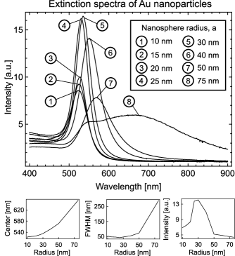
Figure 2: The results of measurement of light extinction in water colloidal solution of Au nanoparticles with radii $a$ indicated in the inset; bottom—extracted red-shift of resonance frequency (left), half-width of the attenuation peak (central) and peak height (right) versus nanosphere radius $a$

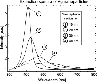
Figure 3: The results of measurement of light extinction in water colloidal solution of Ag nanoparticles with radii $a$ indicated in the inset

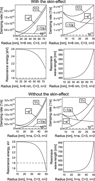
Figure 4: Damping rate (Eq. (32)) of surface plasmons and corresponding resonance shift with respect to nanosphere radius for Au in colloidal water solution with inclusion of screening via skin layer with the depth $h=6$ nm (upper) and without screening (lower); screening (skin-effect) improves fitting with the experimental data—cf. Fig. 2

In the above consideration all irradiating electrons in the sphere were treated equivalently. Note that in surface plasmon oscillations take part all electrons, since it is a translational movement of all collective electrons. In fact some part of electron irradiation is absorbed by other electrons in the system, which reduces outside energy transfer. It can be accounted for in analogy to skin-effect in metals via introducing an effective radiationally active layer with a depth $h$ close to the sphere surface. Thus the factor $\frac{4\pi}{3}(a^{3}-(a-h)^{3})/\frac{4\pi a^{3}}{3}$ can be introduced in the formula (39) to account for screening skin-effect in the metallic nanosphere, with $h\sim\frac{1}{\sigma\omega}$, ($\sigma$—conductivity) as for normal skin-effectabr . Inclusion of screening results thus in reducing of Lorentz friction and in reducing of induced by radiation losses red-shift of resonance, from $a^{3}$ dependence to $a^{2}$, being closer to experimental data in the latter case—cf. Figs 2, 3 and 4. for comparison of $\sim a^{3}$ and $\sim a^{2}$ red-shift of resonance.

IV E-m response of the system of metallic nanospheres

Let us consider number $N_{s}$ of identical metallic nanospheres (with radius $a$) randomly located in the dielectric medium ($\varepsilon\geq 1$) of volume $V$. We assume the metal is simple (as considered in the previous sections) and separation between spheres is sufficiently large to neglect inter-sphere electric interaction. The Hamiltonian of electrons in the system of $N_{s}$ spheres (in ’jellium’ model) has the form: $\hat{H}_{s}=\sum\limits_{l=1}^{N_{s}}\hat{H}_{e}({\bm{r}}_{l})$, where ${\bm{r}}_{l}$ is the position of $l$-th sphere center, $\hat{H}_{e}({\bm{r}}_{l})$ is the electron Hamiltonian of the $l$-th sphere. Thus the total electron wave function $\psi_{e}=\prod\limits_{l=1}^{N_{s}}\Psi_{e}^{l}$, and $i\hbar\frac{\partial\Psi_{e}^{l}}{\partial t}=\hat{H}_{e}({\bm{r}}_{l})\Psi_{e}^{l}$. A density of electrons in the system has the form: $\rho_{s}({\bm{r}},t)=\sum\limits_{l=1}^{N_{s}}\rho({\bm{r}}-{\bm{r}}_{l},t)$, where $\rho({\bm{r}}-{\bm{r}}_{l},t)=<\Psi_{e}^{l}|\sum\limits_{j}\delta({\bm{r}}-{\bm{r}}_{l}-{\bm{r}}_{j})|\Psi_{e}^{l}>$ is the contribution to the total electron density from the $l$th sphere electrons (${\bm{r}}_{j}$ is electron position relative to sphere center).

The space-time Fourier picture of this electron density has the form: $\tilde{\rho}_{s}({\bm{k}},\omega)=\frac{1}{(2\pi)^{4}}\int dtd^{3}re^{-i{\bm{k}}\cdot{\bm{r}}+i\omega t}\rho_{s}({\bm{r}},t)=\tilde{\rho}({\bm{k}},\omega)\sum\limits_{l=1}^{N_{s}}e^{-i{\bm{k}}\cdot{\bm{r}}_{l}}$. According to the notation (23) we have $\tilde{\rho}({\bm{k}},\omega)=\tilde{\rho}_{0}({\bm{k}})\delta(\omega)+\tilde{\rho}_{1}({\bm{k}},\omega)$, with:

$$\begin{array}[]{l}\tilde{\rho}_{0}({\bm{k}})=\frac{1}{(2\pi)^{3}}\int d^{3}r\rho_{0}({\bm{r}})e^{-i{\bm{k}}\cdot{\bm{r}}},\\ \tilde{\rho}_{1}({\bm{k}},\omega)=\frac{1}{(2\pi)^{3}}\sum\limits_{l=1}^{\infty}\sum\limits_{m=-l}^{l}B_{lm}\int d\Omega Y_{lm}(\Omega)e^{-i{\bm{k}}\cdot{\bm{a}}}\frac{\delta(\omega+\omega_{0l})-\delta(\omega-\omega_{0l})}{2i}\\ +\frac{1}{(2\pi)^{3}}\sum\limits_{l=1}^{\infty}\sum\limits_{m=-l}^{l}\sum\limits_{n=1}^{\infty}A_{lm}\left\{n_{e}\frac{(l+1)\omega_{p}^{2}}{l\omega_{p}^{2}-(2l+1)\omega_{nl}^{2}}\int\limits_{0}^{a}dr_{1}\frac{r_{1}^{2+l}}{a^{2l}}j_{l}(k_{nl}r_{1})\int Y_{ln}(\Omega_{1})e^{-i{\bm{k}}\cdot{\bm{a}}}\right.\\ \left.+n_{e}\int\limits_{0}^{a}dr_{1}r_{1}^{2}\int d\Omega_{1}e^{-i{\bm{k}}\cdot{\bm{r}_{1}}}j_{l}(k_{nl}r_{1})Y(\Omega_{1})\right\}\frac{\delta(\omega+\omega_{nl})-\delta(\omega-\omega_{nl})}{2i},\end{array}$$ (40)

here ${\bm{a}}=a\hat{{\bm{r}}}_{1}$, $\hat{{\bm{r}}}=\frac{{\bm{r}}}{r}$. If now one uses the continuity equation, $\frac{\partial\rho_{s}}{\partial t}=div{\bm{j}}_{s}$, or in the Fourier form, ${\bm{k}}\cdot\tilde{\bm{j}}_{s}({\bm{k}},\omega)=\omega\tilde{\rho}_{s}({\bm{k}},\omega)$ (here ${\bm{j}}_{s}$ is the electron current), then one can find: ${\bm{k}}\cdot\tilde{\bm{j}}_{s}({\bm{k}},\omega)=\omega\tilde{\rho_{1}}({\bm{k}},\omega)\sum\limits_{l=1}^{N_{s}}e^{-i{\bm{k}}\cdot{\bm{r}}_{l}}$.

For long wave-length limit ($ka<<1$, which is appropriate for the e-m response of nanospheres; i.e. assuming the ’dipole approximation’, when only linear in $k$ terms remain) we use the following approximations: $e^{-i{\bm{k}}\cdot{\bm{r}}}\simeq 1-i{\bm{k}}\cdot{\bm{r}}$ and ${\bm{k}}\cdot\tilde{\bm{j}}({\bm{k}},\omega)\simeq{\bm{k}}\cdot\tilde{\bm{j}}(0,\omega)$. Thus one can rewrite the continuity equation in the form:

$$\begin{array}[]{l}{\bm{k}}\cdot\tilde{\bm{j}}_{s}(0,\omega)=N_{s}\omega\left\{\sum\limits_{l=1}^{\infty}\sum\limits_{m=-l}^{l}\sum\limits_{n=1}^{\infty}A_{lm}\left[\frac{n_{e}}{(2\pi)^{3}}\int\limits_{0}^{a}dr_{1}r_{1}^{2}j_{l}(k_{nl}r_{1})\int d\Omega_{1}Y_{lm}(\Omega_{1})(-i{\bm{k}}\cdot{\bm{r}}_{1})\right.\right.\\ +\frac{n_{e}}{(2\pi)^{3}}\frac{(l+1)\omega_{p}^{2}}{l\omega_{p}^{2}-(2l+1)\omega_{nl}^{2}}\int\limits_{0}^{a}dr_{1}r_{1}^{l+2}/a^{l}j_{l}(k_{nl}r_{1})\int d\Omega_{1}Y_{lm}(\Omega_{1})\left.(-i{\bm{k}}\cdot{\bm{a}})\right]\frac{\delta(\omega+\omega_{nl})-\delta(\omega-\omega_{nl})}{2i}\\ \left.+\sum\limits_{l=1}^{\infty}\sum\limits_{m=-l}^{l}B_{lm}\frac{1}{(2\pi)^{3}}\int d\Omega_{1}Y_{lm}(\Omega_{1})(-i{\bm{k}}\cdot{\bm{a}})\frac{\delta(\omega+\omega_{0l})-\delta(\omega-\omega_{0l})}{2i}\right\}\\ \end{array}$$ (41)

(as for sufficiently dense nanocomponent system $\sum\limits_{l=1}^{N_{s}}e^{-i{\bm{k}}\cdot{\bm{r}_{l}}}\simeq 1$, and $\int d\Omega Y_{lm}(\Omega)=0$, for $l\geq 1$). Assuming a rapid excitation of all frequencies (${\bm{E}}(t)={\bm{E}}_{0}2\pi\delta(t)$, and thus $\tilde{\bm{E}}(\omega)={\bm{E}}_{0})$ one can write from the Ohm law $-e\tilde{{\bm{j}}}_{s}(0,\omega)=\sigma(\omega){\bm{E}}_{0}$, and next, for ${\bm{E}}_{0}$ in $z$-th direction, ${\bm{k}}\cdot{\bm{E}}_{0}=cos\Theta,\;{\bm{k}}\cdot{\bm{r}}_{1}=kr_{1}\frac{4\pi}{3}\left\{cos\Theta Y_{10}(\Omega_{1})+\frac{1}{\sqrt{2}}sin(\Theta)[Y_{11}(\Omega_{1})+Y_{1-1}(\Omega_{1})]\right\}$, and ${\bm{k}}\cdot{\bm{a}}=ka\frac{4\pi}{3}\left\{cos\Theta Y_{10}(\Omega_{1}^{\prime})+\frac{1}{\sqrt{2}}sin(\Theta)[Y_{11}(\Omega_{1}^{\prime})+Y_{1-1}(\Omega_{1}^{\prime})]\right\}$, where $\Omega_{1}=(\theta_{1},\phi_{1})$ and $\Omega_{1}^{\prime}=(\theta_{1}^{\prime},\phi_{1}^{\prime})$. Thus one can obtain:

$$\begin{array}[]{l}\sigma(\omega)E_{0}kcos\Theta=\frac{N_{s}|e|\omega k}{2(2\pi)^{3}}\sqrt{\frac{4\pi}{3}}\left\{\sum\limits_{n=1}^{\infty}n_{e}\int\limits_{0}^{a}r_{1}^{3}dr_{1}j_{1}(k_{1n}r_{1})\right.\\ \left(1+\frac{2\omega_{p}^{2}}{\omega_{p}^{2}-3\omega_{n1}^{2}}\right)\left([A_{10}cos\theta+sin\theta\sqrt{\frac{1}{2}}(A_{11}+A_{1-1})](\delta(\omega-\omega_{n1})-\delta(\omega+\omega_{n1}))\right)\\ \left.+a[B_{10}cos\theta+sin\Theta\sqrt{\frac{1}{2}}(B_{11}+B_{1-1})]\left(\delta(\omega-\omega_{01})-\delta(\omega+\omega_{01})\right)\right\},\\ \end{array}$$ (42)

from which $A_{11}+A_{1-1}=B_{11}+B_{1-1}=0$, while $A_{10}=\mu E_{0}$ and $B_{10}=\nu n_{e}a^{3}E_{0}$ (the constants $\mu,\nu$ will be determined later). From the above it follows:

$$\begin{array}[]{l}\sigma(\omega)=\frac{|e|N_{s}\omega}{2(2\pi)^{3}}\sqrt{\frac{4\pi}{3}}n_{e}a^{4}\left\{\nu(\delta(\omega-\omega_{01})-\delta(\omega+\omega_{01}))\right.\\ +\left.\mu\sum\limits_{n=1}^{\infty}\frac{3}{(2k_{T}^{2}a^{2}+3x_{n1}^{2})x_{n1}^{2}}\int\limits_{0}^{x_{n1}}x^{3}dxj_{1}(x)(\delta(\omega-\omega_{n1})-\delta(\omega+\omega_{n1}))\right\},\end{array}$$ (43)

where $\omega_{n1}^{2}=\omega_{p}^{2}(1+x_{n1}^{2}/(k_{T}a^{2}))$. Via the formula for $\sigma$ one can now derive the dielectric response function $\varepsilon(\omega)=\varepsilon^{\prime}(\omega)+i\varepsilon^{\prime\prime}(\omega)$, with $\varepsilon^{\prime\prime}(\omega)=\frac{4\pi}{\omega}\sigma(\omega)$ and $\varepsilon^{\prime}(\omega)=\varepsilon+\frac{1}{\pi}{\cal{P}}\int\limits_{-\infty}^{+\infty}dx\frac{\varepsilon^{\prime\prime}(x)}{x-\omega}$:

$$\begin{array}[]{l}\varepsilon^{\prime\prime}(\omega)=\frac{|e|N_{s}n_{e}a^{4}}{4\pi^{2}}\sqrt{\frac{4\pi}{3}}\left\{\nu(\delta(\omega-\omega_{01})-\delta(\omega+\omega_{01}))\right.\\ \left.+\mu\sum\limits_{n=1}^{\infty}\frac{3}{(2k_{T}a^{2}+3x_{n1}^{2})x_{n1}^{2}}\int\limits_{0}^{x_{n1}}dxx^{3}j_{1}(x)(\delta(\omega-\omega_{n1})-\delta(\omega+\omega_{n1}))\right\},\\ \end{array}$$ (44)

and

$$\begin{array}[]{l}\varepsilon^{\prime}(\omega)=\varepsilon+\frac{|e|N_{s}n_{e}a^{4}}{2\pi^{2}}\sqrt{\frac{4\pi}{3}}\left\{\nu{\cal P}\frac{\omega_{01}}{\omega_{01}^{2}-\omega^{2}}\right.\\ \left.+\mu\sum\limits_{n=1}^{\infty}\frac{3}{(2k_{T}a^{2}+3x_{n1}^{2})x_{n1}^{2}}\int\limits_{0}^{x_{n1}}dxx^{2}j_{1}(x){\cal P}\frac{\omega_{n1}}{\omega_{n1}^{2}-\omega^{2}}\right\}.\\ \end{array}$$ (45)

One can determine now the constants $\mu,\nu$ using the sum rule: $\int\limits_{0}^{\infty}d\omega\omega\varepsilon^{\prime\prime}(\omega)=\frac{n2\pi^{2}e^{2}}{m}$, where $n=\frac{N}{V}=\frac{N_{s}V_{0}n_{e}}{V}$, (here, $V$—the volume of the whole system, $V_{0}$—the volume of the single nanosphere), and the static value of the dielectric response of the system $\varepsilon(0)=\varepsilon+8\int\limits_{0}^{\infty}d\omega{\cal P}\frac{\sigma(\omega)}{\omega^{2}}$ (assumed to be known). These conditions give:

$$\mu=\frac{\omega_{p}^{2}c_{0}}{u\omega_{01}[\alpha_{1}-\alpha_{2}]}\left(1-\frac{\varepsilon(0)-\varepsilon}{3c_{0}\varepsilon}\right),\;\nu=\frac{\omega_{p}^{2}c_{0}}{u\omega_{01}[\alpha_{1}-\alpha_{2}]}\left(\alpha_{1}\frac{\varepsilon(0)-\varepsilon}{3c_{0}\varepsilon}-\alpha_{2}\right),$$ (46)

where $\alpha_{1}=\sum\limits_{n=1}^{\infty}\frac{3}{(2k_{T}^{2}a^{2}+3x_{n1}^{2})x_{n1}^{2}}\int\limits_{0}^{x_{n1}}dxx^{3}j_{1}(x)\frac{\omega_{n1}}{\omega_{01}}$, $\alpha_{2}=\sum\limits_{n=1}^{\infty}\frac{3}{(2k_{T}^{2}a^{2}+3x_{n1}^{2})x_{n1}^{2}}\int\limits_{0}^{x_{n1}}dxx^{3}j_{1}(x)\frac{\omega_{01}}{\omega_{n1}}$,
$c_{0}=N_{s}\frac{V_{0}}{V}$, $u=\frac{4|e|n_{e}N_{s}a^{4}}{(2\pi)^{3}}\sqrt{\frac{4\pi}{3}}$,.

By introducing the oscillator strength $f(\omega)=\frac{2\omega\varepsilon^{\prime\prime}(\omega)}{\pi c_{0}\omega_{p}^{2}}$, one can express the dipole-type dielectric response of the considered metallically nanomodified system in a more conventional form:

$$\varepsilon(\omega)=\varepsilon^{\prime}(\omega)+i\varepsilon^{\prime\prime}(\omega)=\varepsilon+c_{0}\omega_{p}^{2}\sum\limits_{n=0}^{\infty}\frac{f_{n}}{2\omega_{n1}}\left[\frac{1}{\omega_{n1}-\omega-i\epsilon}+\frac{1}{\omega_{n1}+\omega+i\epsilon}\right],$$ (47)

where $\epsilon=0+$, $f(\omega)=\sum\limits_{n=0}^{\infty}f_{n}[\delta(\omega-\omega_{n1})+\delta(\omega+\omega_{n1})]$, $f_{0}=\frac{1}{\alpha_{1}-\alpha_{2}}\left(\frac{\varepsilon(0)-\varepsilon_{0}}{3c_{0}\varepsilon_{0}}\alpha_{1}-\alpha_{2}\right)$, $f_{n}=\frac{1}{\alpha_{1}-\alpha_{2}}\left(1-\frac{\varepsilon(0)-\varepsilon_{0}}{3c_{0}\varepsilon_{0}}\right)\frac{3}{(2k_{t}^{2}a^{2}+3x_{n1}^{2})x_{n1}^{2}}\frac{\omega_{n1}}{\omega_{01}}\int\limits_{0}^{x_{n1}}dxx^{3}j_{1}(x)$, $\int\limits_{0}^{\infty}d\omega f(\omega)=\sum\limits_{n=0}^{\infty}f_{n}=1$.

We can include attenuation (also due to irradiation losses), of dipole excitations ($l=1$), via the damping term $\frac{2}{\tau}\frac{\partial\rho_{1}({\bm{r}},t)}{\partial t}$ in oscillator-type equation for plasmons (which can be added to left-hand-side of Eq. (13) and assuming that all modes are damped with the same attenuation time $\tau$). Thus the time-dependent solution of such modified equation attains the form as given by Eq. (20) with the factor $e^{-t/\tau}$, and with the shifted frequency $\omega^{\prime}_{n}=\sqrt{\omega_{n}^{2}-\frac{1}{\tau^{2}}}$. Similarly to the equation for the surface plasmons, Eq. (14), can be added (to its left-hand-side) the damping term $\frac{2}{\tau}\frac{\partial\rho_{2}({\bm{r}},t)}{\partial t}$. It leads to the factor $e^{-t/\tau}$ for the first part of the solution (21) (and simultaneously shifted frequency $\omega^{\prime}_{l0}=\sqrt{\omega_{l0}^{2}-\frac{1}{\tau^{2}}}$), and the second term of Eq. (21) acquires the additional factor $e^{-t/\tau}$ (and shifted frequency $\omega^{\prime}_{n}=\sqrt{\omega_{n}^{2}-\frac{1}{\tau^{2}}}$). The corresponding change in the dipole-type ($l=1$) e-m response function (47) resolves thus to the following expression:

$$\varepsilon(\omega)=\varepsilon^{\prime}(\omega)+i\varepsilon^{\prime\prime}(\omega)=\varepsilon+c_{0}\omega_{p}^{2}\sum\limits_{n=0}^{\infty}\frac{f_{n}}{2\omega^{\prime}_{n1}}\left[\frac{1}{\omega^{\prime}_{n1}-\omega-\frac{i}{\tau}}+\frac{1}{\omega^{\prime}_{n1}+\omega+\frac{i}{\tau}}\right].$$ (48)

The above equation can be rewritten as follows:

$$\varepsilon^{\prime}(\omega)=\varepsilon+c_{0}\omega_{p}^{2}\sum\limits_{n=0}^{\infty}\frac{f_{n}}{2\omega^{\prime}_{n1}}\left[\frac{\omega^{\prime}_{n1}-\omega}{(\omega^{\prime}_{n1}-\omega)^{2}+\frac{1}{\tau^{2}}}+\frac{\omega^{\prime}_{n1}+\omega}{(\omega^{\prime}_{n1}+\omega)^{2}+\frac{1}{\tau^{2}}}\right]$$ (49)

and

$$\varepsilon^{\prime\prime}(\omega)=c_{0}\omega_{p}^{2}\sum\limits_{n=0}^{\infty}\frac{f_{n}}{2\omega^{\prime}_{n1}\tau}\left[\frac{1}{(\omega^{{}^{\prime}}_{n1}-\omega)^{2}+\frac{1}{\tau^{2}}}-\frac{1}{(\omega^{{}^{\prime}}_{n1}+\omega)^{2}+\frac{1}{\tau^{2}}}\right].$$ (50)

V Measurement of the dipole surface plasmon frequencies in nanoparticles with variation of their radius

To determine the plasmon frequencies in metal nanoparticles as a function of the nanoparticle radius, extinction spectra of colloidal solution of Au and Ag nanoparticles with radii ranging form 10 nm to 75 nm for Au, and from 10 nm to 40 nm for Ag, respectively, were measured. The nanoparticles, prepared as a water colloidal solution with an average size distribution not exceeding 8% and an almost constant total mass per ml independent of the particle radii, were obtained from British Biocell International. The particular data of the Au nanoparticles are listed in Tab. 1.

Tab. 1. Nanoparticle data for Au colloidal solutions
nominal nanosphere radius [nm]	10	15.	20	25	30	40	50	75
average nanosphere radius [nm]	10.2	15.55	20.55	24.65	29.35	39	49.45	77.15
particle density [109/ml]	700	200	90	45	26	11	5.6	1.7
total volume [1015 nm3/ml]	3.11	3.15	3.27	2.82	2.75	2.73	2.84	3.27

The extinction spectra were measured using a xenon lamp operated at 150 W in combination with a Monospek 1000 monochrometer, providing monochromatic light at wavelengths from 300 nm to 900 nm. To accommodate for the response of the aqueous environment, the cuvette containing the colloidal solution and the lamp spectrum, reference measurements were performed to which the extinction spectra are normalized. The extinction coefficient shown in Figs. 2 and 3 is defined as the fraction $T_{C}/T_{Au,Ag}$, where $T_{C}$ is the light intensity transmitted through the cuvette containing de-ionized water and $T_{Au,Ag}$ light intensity transmitted through the cuvette containing Au or Ag nanoparticle colloidal solutions.

The results are presented in Fig. 2 for Au and in Fig. 3 for Ag, respectively. The red-shift of the resonant frequency with growth of nanosphere radius is clearly noticeable. This is accompanied by the broadening of the attenuation peak and variation of peak height (at the beginning growth and next lowering of the peak height). These features are collected in the Fig. 2 (bottom) for Au, where the position of the center of extinction peak, its half-width and height are plotted versus the nanosphere radius.

For nanoparticles of gold, silver and copper in the air, in water and in a colloidal solution, one can find $a_{0}\sim 10-14$ nm (cf. Eq. (33), Fig. 1 and Fig. 4), i.e., the radius of nanosphere corresponding to minimal damping, which well corresponds to experimental dataccc ; scharte . It is a cross-over point for the resonance red-shift versus $a$. For $a>a_{0}$ damping increases due to Lorentz friction (proportionally to $a^{3}$, or after inclusion of screening, proportionally to $a^{2}$) but for $a<a_{0}$ damping due to electron scattering dominates and causes opposite behavior—enhancement of damping with lowering radius (proportional to $\frac{1}{a}$, in agreement with experimental observationsatwater ; ccc ), which leads to cross-over of resonance red-shift dependence on $a$.

Surface plasmon oscillations cause attenuation of the incident e-m radiation where the maximum of attenuation is at the resonant frequencyjac $\omega_{1}=\sqrt{\omega_{1}^{2}-\frac{1}{\tau^{2}}}$. This frequency diminishes with growth of $a$, for $a>a_{0}$ according to Eq. (32), which agrees well with the experimental measurements for Au and Ag presented in Figs 2 and 3 and in Tabs 2 and 3 (after inclusion of screening via skin-effect type correction—cf. Fig. 4).

Tab. 2. Resonant frequency for e-m wave attenuation in Au nanospheres
radius of nanospheres [nm]	10	15	20	25	30	40	50	75
$\hbar\omega_{1}^{\prime}$ (experiment) [eV]	2.371	2.362	2.357	2.340	2.316	2.248	2.172	1.895
$\hbar\omega_{1}^{\prime}$ (theory, $h=a$) [eV], $n_{0}=1.4$	3.72	3.716	3.71	3.69	3.66	2.41	2.37	XXX
$\hbar\omega_{1}^{\prime}$ (theory, $h=a$) [eV], $n_{0}=2$	2.601	2.60	2.59	2.58	2.56	2.38	1.64	XXX
$\hbar\omega_{1}^{\prime}$ (theory, $h=6$ nm) [eV], $n_{0}=2$	2.601	2.600	2.599	2.595	2.58	2.55	2.47	1.84

($C=2$, $v_{F}=1.396\cdot 10^{6}$ m/s, $\lambda_{B}=5.3\cdot 10^{-8}$ m, [cf. Eq. (32)], $\omega_{p}=1.371\cdot 10^{16}$ 1/s, $\omega_{1}=3.96\cdot 10^{15}$ 1/s [for n=2]) XXX—overdamped oscillations;

Tab. 3. Resonant frequency for e-m wave attenuation in Ag nanospheres
radius of nanospheres [nm]	10	20	30	40
$\hbar\omega_{1}^{\prime}$ (experiment) [eV]	3.024	2.911	2.633	2.385
$\hbar\omega_{1}^{\prime}$ (theory, $h=a$) [eV], $n_{0}=1.4$	3.71	2.70	2.66	2.41
$\hbar\omega_{1}^{\prime}$ (theory, $h=a$) [eV], $n_{0}=2$	2.61	2.60	2.56	2.382
$\hbar\omega_{1}^{\prime}$ (theory, $h=8$ nm) [eV], $n_{0}=2$	2.60	2.59	2.58	2.55

(C=2, $v_{F}=1.393\cdot 10^{6}$ m/s, $\lambda_{B}=5.3\cdot 10^{-8}$ m, [cf. Eq. (32)], $\omega_{p}=1.37\cdot 10^{16}$ 1/s, $\omega_{1}=7.89\cdot 10^{15}$ 1/s [for n=1])

The observed behavior well corresponds with the formula (32) with the additional skin-effect factor in the last term $\frac{4\pi}{3}(a^{3}-(a-h)^{3})/\frac{4\pi}{3}a^{3}$ (reducing $a^{3}$ to $a^{2}$ radius dependence), which gives the damping rate $\frac{1}{\tau}$ for surface dipole plasmons versus $a$. This damping leads to Lorentzian shape of attenuation peak (in response function), $\frac{1/\tau^{2}}{(\omega-\omega^{\prime})^{2}+1/\tau^{2}}$ with central position at frequency $\omega^{\prime}=\sqrt{\omega_{1}^{2}-1/\tau^{2}}$. As $1/\tau$ scales as $a^{2}$, after inclusion of screening—cf. Fig. 4, it is dominating contribution to the value given by Eq. (32) for $a\geq 20$ nm (in agreement with the experiment). Inclusion of screening (Fig. 4) reduces irradiation-induced damping of plasmons at limiting large values of nanosphere radius and allows to avoid overdamped regime in this case, which is entered by unscreened $a^{3}$ damping rate dependence at $a\sim 75$ nm (cf. Tab. 2). The agreement between the model and the experimental data suggests that for the $a$ dependent red-shift of resonance frequency of surface plasmons in metallic nanoparticles of large size ($10<a<75$ nm) responsible are plasmon energy losses caused by Lorentz friction.

VI Conclusions

We have analyzed red-shift of Mie frequency of dipole surface plasmon oscillations in large metallic nanospheres, with radius beyond 10 nm. For this region of metallic cluster size the dominating channel of plasmon damping starts to be radiation loss due to Lorentz friction. At approximately 10 nm for nanosphere radius the cross-over point of red-shift versus nanosphere radius occurs. For lower radii the $\frac{1}{a}$ rule dominates describing scattering Fermi type mechanisms of damping, for higher radii the damping due to Lorentz friction, with radius dependence $\sim a^{3}$ (or $\sim a^{2}$ when screening is included), prevails and quickly completely dominates plasmon attenuation. The resulting red-shift of damped harmonic oscillation well reproduces the experimentally observed resonance positions with respect to metallic sphere size. We have measured the resonance positions via observation of extinction of light in water colloidal solutions of Au nanospheres with radii between 10 and 75 nm, and Ag with radii between 10 and 40 nm. The theoretical predictions well fit to the experimental behavior, especially if include corrections due to radiation screening of skin-effect type. The resulting $a^{2}$ scaling well reproduces the experimental curves for skin-depth of order of 6 nm (for Au). At the limiting value of metallic nanosphere radius ($a>75$ nm) an almost overdamped oscillation regime is expected from theoretical analysis, earlier for Ag than for Au, due to bigger conductivity in Au and thus stronger reducing damping than in Ag. In experiment the corresponding large red-shift in the almost overdamped regime is observed for both Au and Ag. Moreover, the first volume mode with original energy above $\hbar\omega_{p}$ (bulk volume plasmon frequency) in the case of an almost overdamped regime is strongly red-shifted and emerges in extinction features as an additional smaller peak on the left side of surface plasmon peak for sufficiently large nanospheres, when dipole approximation is not exact.

Appendix A Analytical solution of plasmon equations for the nanosphere

Let us solve first the Eq. (16), assuming the solution in the form:

$$\delta\rho_{1}({\bm{r},t})=n_{e}\left[f_{1}(r)+F({\bm{r}},t)\right],\;for\;r<a.$$ (51)

Eq. (16) resolves thus into:

$$\begin{array}[]{l}\nabla^{2}f_{1}(r)-k_{T}^{2}f_{1}(r)=0,\\ \frac{\partial^{2}F({\bm{r}},t)}{\partial t^{2}}+\frac{2}{\tau_{0}}\frac{\partial F({\bm{r}},t)}{\partial t}=\frac{v_{F}^{2}}{3}\nabla^{2}F({\bm{r}},t)-\omega_{p}^{2}F({\bm{r}},t).\\ \end{array}$$ (52)

The solution for function $f_{1}(r)$ (nonsingular at $r=0$) has thus the form:

$$f_{1}(r)=\alpha\frac{e^{-k_{T}a}}{k_{T}r}\left(e^{-k_{T}r}-e^{k_{T}r}\right),$$ (53)

where $\alpha$ is a constant, $k_{T}=\sqrt{\frac{6\pi n_{e}e^{2}}{\epsilon_{F}}}=\sqrt{\frac{3\omega_{p}^{2}}{v_{F}^{2}}}\;$ ($k_{T}$ is the inverse Thomas-Fermi radius), $\omega_{p}=\sqrt{\frac{4\pi n_{e}e^{2}}{m}}\;$ (bulk plasmon frequency).

Since we assumed $F({\bm{r}},0)=0$, then for function $F({\bm{r}},t)$ the solution can be taken as,

$$F({\bm{r}},t)=F_{\omega}({\bm{r}})sin(\omega^{\prime}t)e^{-\tau_{0}t}$$ (54)

where $\omega^{\prime}=\sqrt{\omega^{2}+1/\tau_{0}^{2}}$. $F_{\omega}({\bm{r}})$ satisfies the equation (Helmholtz equation):

$$\nabla^{2}F_{\omega}({\bm{r}})+k^{2}F_{\omega}({\bm{r}})=0,$$ (55)

with $k^{2}=\frac{\omega^{2}-\omega_{p}^{2}}{v_{F}^{2}/3}$. A solution of the above equation, nonsingular at $r=0$, is as follows:

$$F_{\omega}({\bm{r}})=Aj_{l}(kr)Y_{lm}(\Omega),$$ (56)

where $A$ is a constant, $j_{l}(\xi)=\sqrt{\pi/(2\xi)}I_{l+1/2}(\xi)$ the spherical Bessel function [$I_{n}(\xi)$ the Bessel function of the first order], and $Y_{lm}(\Omega)$ the spherical function ($\Omega$ the spherical angle). Owing to the semiclassical boundary condition, $F({\bm{r}},t)|_{r=a}=0$, one has to demand $j_{l}(ka)=0$, which leads to the discrete values of $k=k_{nl}=x_{nl}/a$, (where $x_{nl},\;\;n=1,2,3...$, are nodes of $j_{l}$), and next to the discretization of self-frequencies:

$$\omega_{nl}^{2}=\omega_{p}^{2}\left(1+\frac{x_{nl}^{2}}{k_{T}^{2}a^{2}}\right).$$ (57)

The general solution for $F({\bm{r}},t)$ attains thus the form

$$F({\bm{r}},t)=\sum\limits_{l=0}^{\infty}\sum\limits_{m=-l}^{l}\sum\limits_{n=1}^{\infty}A_{lmn}j_{l}(k_{nl}r)Y_{lm}(\Omega)sin(\omega^{\prime}_{nl}t)e^{-\tau_{0}t}.$$ (58)

A solution of Eq. (17) we represent as:

$$\delta\rho_{2}({\bm{r},t})=n_{e}f_{2}(r)+\sigma(\Omega,t)\delta(r+\epsilon-a),\;for\;r\geq a,\;(r\rightarrow a+,i.e.\epsilon\rightarrow 0).$$ (59)

The neutrality condition, $\int\rho({\bm{r}},t)d^{3}r=N_{e}$, with $\delta\rho_{2}({\bm{r}},t)=\sigma(\omega,t)\delta(a+\epsilon-r)+n_{e}f_{2}(r),(\;\epsilon\rightarrow 0)$, can be rewritten as follows: $-\int\limits_{0}^{a}drr^{2}f_{1}(r)=\int\limits_{a}^{\infty}drr^{2}f_{2}(r)$, $\int\limits_{0}^{a}d^{3}rF({\bm{r}},t)=0$, $\int d\Omega\sigma(\Omega,t)=0$. Taking into account also the continuity condition on the surface, $1+f_{1}(a)=f_{2}(a)$, one can obtain: $f_{2}(r)=\beta e^{-k_{T}(r-a)}/(k_{T}r)$ and it is possible to fit $\alpha$ (cf. Eq. (53)) and $\beta$ constants: $\alpha=\frac{k_{T}a+1}{2}$, $\beta=k_{T}a-\frac{k_{T}a+1}{2}\left(1-e^{-2k_{T}a}\right)$, which gives Eqs (19).

From the condition $\int\limits_{0}^{a}d^{3}rF({\bm{r}},t)=0$ and from Eq. (58) it follows that $A_{00n}=0$, (because of $\int d\Omega Y_{lm}(\omega)=4\pi\delta_{l0}\delta_{m0}$).

In order to remove the Dirac delta functions we integrate both sides of the Eq. (17) with respect to the radius length ($\int\limits_{0}^{\infty}r^{2}dr...$) and then we take the limit to the sphere surface, $\epsilon\rightarrow 0$. It results in the following equation for surface plasmons:

$$\begin{array}[]{l}\frac{\partial^{2}\sigma(\Omega,t)}{\partial t^{2}}+\frac{2}{\tau_{0}}\frac{\partial\sigma(\Omega,t)}{\partial t}=-\sum\limits_{l=0}^{\infty}\sum\limits_{m=-l}^{l}\omega_{0l}^{2}Y_{lm}(\Omega)\int d\Omega_{1}\sigma(\Omega_{1},t)Y^{*}_{lm}(\Omega_{1})\\ +\omega_{p}^{2}n_{e}\sum\limits_{l=0}^{\infty}\sum\limits_{m=-l}^{l}\sum\limits_{n=1}^{\infty}A_{lmn}\frac{l+1}{2l+1}Y_{lm}(\Omega)\int\limits_{0}^{a}dr_{1}\frac{r_{1}^{l+2}}{a^{l+2}}j_{l}(k_{nl}r_{1})sin(\omega_{nl}t),\\ +\frac{en_{e}}{m}\sqrt{4\pi/3}\left[E_{z}(t)Y_{10}(\Omega)+\sqrt{2}E_{x}(t)Y_{11}(\Omega)+\sqrt{2}E_{y}(t)Y_{1-1}(\Omega)\right],\end{array}$$ (60)

where $\omega_{0l}^{2}=\omega_{p}^{2}\frac{l}{2l+1}$. In derivation of the above equation the following formulae were exploited, (for $a<r_{1}$):

$$\frac{\partial}{\partial a}\frac{1}{\sqrt{a^{2}+r_{1}^{2}-2ar_{1}cos\gamma}}=\frac{\partial}{\partial a}\sum\limits_{l=0}^{\infty}\frac{a^{l}}{r_{1}^{l+1}}P_{l}(cos\gamma)=\sum\limits_{l=0}^{\infty}\frac{la^{l-1}}{r_{1}^{l+1}}P_{l}(cos\gamma),$$ (61)

where $P_{l}(cos\gamma)$ is the Legendre polynomial [$P_{l}(cos\gamma)=\frac{4\pi}{2l+1}\sum\limits_{m=-l}^{l}Y_{lm}(\Omega)Y^{*}_{lm}(\Omega_{1})$], $\gamma$ is an angle between vectors ${\bm{a}}=a\hat{\bm{r}}$ and ${\bm{r}}_{1}$, and (for $a>r_{1}$):

$$\frac{\partial}{\partial a}\frac{1}{\sqrt{a^{2}+r_{1}^{2}-2ar_{1}cos\gamma}}=\frac{\partial}{\partial a}\sum\limits_{l=0}^{\infty}\frac{r_{1}^{l}}{a^{l+1}}P_{l}(cos\gamma)=-\sum\limits_{l=0}^{\infty}\sum\limits_{m=-l}^{l}4\pi\frac{l+1}{2l+1}\frac{r_{1}^{l}}{a^{l+2}}Y_{lm}(\Omega)Y^{*}_{lm}(\Omega_{1}).$$ (62)

Taking into account the spherical symmetry, one can assume the solution of the Eq. (60) in the form:

$$\sigma(\Omega,t)=\sum\limits_{l=0}^{\infty}\sum\limits_{m=-l}^{l}q_{lm}(t)Y_{lm}(\Omega).$$ (63)

From the condition $\int\sigma(\omega t)d\Omega=0$ it follows that $q_{00}=0$. Taking into account the initial condition $\sigma(\omega,0)=0$ we get (for $l\geq 1$),

$$\begin{array}[]{l}q_{lm}(t)=\frac{B_{lm}}{a^{2}}sin(\omega_{0l}^{\prime}t)e^{-t/\tau_{0}}(1-\delta_{l1})+Q_{1m}(t)\delta_{l1}\\ +\sum\limits_{n=1}^{\infty}A_{lmn}\frac{(l+1)\omega_{p}^{2}}{l\omega_{p}^{2}-(2l+1)\omega_{nl}^{2}}n_{e}\int\limits_{0}^{a}dr_{1}\frac{r_{1}^{l+2}}{a^{l+2}}j_{l}(k_{nl}r_{1})sin(\omega_{nl}^{\prime}t)e^{-t/\tau_{0}},\\ \end{array}$$ (64)

where $\omega_{0l}^{\prime}=\sqrt{\omega_{0l}^{2}-1/\tau_{0}^{2}}$ and $Q_{1m}(t)$ satisfies the equation:

$$\frac{\partial^{2}Q_{1m}(t}{\partial t^{2}}+\frac{2}{\tau_{0}}\frac{\partial Q_{1m}(t)}{\partial t}+\omega_{01}^{2}Q_{1m}(t)=\frac{en_{e}}{m}\sqrt{4\pi/3}\left[E_{z}(t)\delta_{m0}+\sqrt{2}E_{x}(t)\delta_{m1}+\sqrt{2}E_{y}(t)\delta_{m-1}\right].$$ (65)

Thus $\sigma(\omega,t)$ attains the form:

$$\begin{array}[]{l}\sigma(\Omega,t)=\sum\limits_{l=2}^{\infty}\sum\limits_{m=-l}^{l}Y_{lm}(\Omega)\frac{B_{lm}}{a^{2}}sin(\omega_{0l}^{\prime}t)e^{-t/\tau_{0}}+\sum\limits_{m=-1}^{1}Q_{1m}(t)Y_{1m}(\Omega)\\ +\sum\limits_{l=1}^{\infty}\sum\limits_{m=-l}^{l}\sum\limits_{n=1}^{\infty}A_{nlm}\frac{(l+1)\omega_{p}^{2}}{l\omega_{p}^{2}-(2l+1)\omega_{nl}^{2}}Y_{lm}(\Omega)n_{e}\int\limits_{0}^{a}dr_{1}\frac{r_{1}^{l+2}}{a^{l+2}}j_{l}(k_{nl}r_{1})sin(\omega_{nl}^{\prime}t)e^{-t/\tau_{0}}.\\ \end{array}$$ (66)

References

- (1) S. Pillai, K. B. Catchpole, T. Trupke, G. Zhang, J, Zhao, and M. A. Green, Appl. Phys. Let., 88, 161102 (2006)
- (2) M. Westphalen, U. Kreibig, J. Rostalski, H. Lüth, and D. Meissner, Sol. Energy Mater. Sol. Cells 61, 97 (2000); M. Gratzel, J. Photochem. Photobiol. C: Photochem. Rev. 4, 145 (2003)
- (3) H. R. Stuart and D. G. Hall, Appl. Phys. Lett. 73, 3815 (1998); H. R. Stuart and D. G. Hall, Phys. Rev. Lett. 80, 5663 (1998); H. R. Stuart and D. G. Hall, Appl. Phys. Lett. 69, 2327 (1996)
- (4) D. M. Schaadt, B. Feng, and E. T. Yu, Appl. Phys. Lett. 86, 063106 (2005)
- (5) K. Okamoto, I. Niki, A. Shvartser, Y. Narukawa, T. Mukai, and A. Scherter, Nature Mat. 3, 661 (2004); K. Okamoto, I. Niki, A. Scherer, Y. Narukawa, T. Mukai, and Y. Kawakami, Appl. Phys. Lett. 87, 071102 (2005)
- (6) C. Wen, K. Ishikawa, M. Kishima, K. Yamada, Sol. Cells 61, 339 (2000)
- (7) L. Lalanne, J. P. Hugonin, Nature Phys. 2, 551 (2006)
- (8) A.V. Zayats, I. I. Smolyaninov, and A. A. Maradudin, Phys. Rep. 408, 131 (2005)
- (9) S.A. Mayer, Plasmonics: Fundamentals and Applications, Springer VL 2007
- (10) W. L. Barnes, A. Dereux, and T. W. Ebbesen, Nature 424, 824 (2003)
- (11) C. Burda, X. Chen, R. Narayanan, M. El-Sayed, Chem. Rev. 105, 1025 (2005)
- (12) A. B. Migdal, J. Phys. USSR 8, 331 (1944)
- (13) H. von Steiwedel and J. H. D. Jensen, Z. Naturforsh. A 5, 413 (1950)
- (14) M. Godhaber and E. Teller, Phys. Rev. ‘74, 1046 (1948)
- (15) M. Brack, Rev. of Mod. Phys. 65, 677 (1993)
- (16) W. Ekardt, Phys. Rev B 31, 6360 (1985)
- (17) G. Weick, R. A. Molina, D. Weinmann, and R. A. Jalabert, Phys. Rev. B 72, 115410 (2005)
- (18) V. V. Kresin, Phys. Rep. 220, 1 (1992)
- (19) G. Mie, Ann. Phys. 25, 329 (1908)
- (20) G. Weick, G. L. Ingold, R. A. Jalabert, and D. Weinmann, Phys. Rev. B 74, 165421 (2006)
- (21) L. Serra, F. Garcias, M. Barranco, N. Barberan, and J. Navarro , Phys. Rev. B 41, 3434 (1990)
- (22) M. Brack, Phys. Rev. B 39, 3533 (1989)
- (23) W. Ekardt, Phys. Rev. Lett. 52, 1925 (1984)
- (24) C.F. Bohren and D.R. Huffman, Absorption and Scattering of Light by Small Particles, Wiley, New York (1983); U. Kreibig and M. Vollmer, Optical Properties of Metal Clusters, Springer, Berlin (1995); J. I. Petrov, Physics of Small Particles, Nauka, Moscow (1984)
- (25) L. D. Landau and E. M. Lifshitz, Field Theory, Nauka, Moscow (1973) (in Russian)
- (26) D. Pines, Elementary Excitations in Solids, ABP Perseus Books, Massachusetts (1999)
- (27) D. Pines and D. Bohm, Phys. Rev. 85, 338 (1952); D. Bohm and D. Pines, Phys. Rev. 92, 609 (1953)
- (28) L. Jacak, J. Krasnyj, and A. Chepok, Fizika Niskich Temp. 33, (2009)
- (29) M. L. Brongersma, J. W. Hartman, and H. A. Atwater, Phys. Rev. B 62, R16356 (2000)
- (30) U. Kreibig and L. Genzel, Surf. Sci., 156, 678, (1985)
- (31) A. A. Abrikosov, Osnovy tieorii metalov, Nauka, Moscow (1987)
- (32) F. Stietz, I. Bosbach, T. Wenzel, T. Vartanyan, A. Goldmann, and F. Träger, Phys. Rev. Lett., 84, 5644 (2000)
- (33) M. Scharte, R. Porath, T. Ohms, M. Aeschlimann, J. R. Krenn, H. Ditlbacher, F. R. Aussenegg, and A. Liebsch, Appl. Phys. B: Laser Opt. 73, 305 (2001)