Sparse Recovery from Combined Fusion Frame Measurements

Abstract

Sparse representations have emerged as a powerful tool in signal and information processing, culminated by the success of new acquisition and processing techniques such as Compressed Sensing (CS). Fusion frames are very rich new signal representation methods that use collections of subspaces instead of vectors to represent signals. This work combines these exciting fields to introduce a new sparsity model for fusion frames. Signals that are sparse under the new model can be compressively sampled and uniquely reconstructed in ways similar to sparse signals using standard CS. The combination provides a promising new set of mathematical tools and signal models useful in a variety of applications. With the new model, a sparse signal has energy in very few of the subspaces of the fusion frame, although it does not need to be sparse within each of the subspaces it occupies. This sparsity model is captured using a mixed $\ell_{1}/\ell_{2}$ norm for fusion frames.

A signal sparse in a fusion frame can be sampled using very few random projections and exactly reconstructed using a convex optimization that minimizes this mixed $\ell_{1}/\ell_{2}$ norm. The provided sampling conditions generalize coherence and RIP conditions used in standard CS theory. It is demonstrated that they are sufficient to guarantee sparse recovery of any signal sparse in our model. Moreover, a probabilistic analysis is provided using a stochastic model on the sparse signal that shows that under very mild conditions the probability of recovery failure decays exponentially with increasing dimension of the subspaces.

I Introduction

Compressed Sensing (CS) has recently emerged as a very powerful field in signal processing, enabling the acquisition of signals at rates much lower than previously thought possible [1, 2]. To achieve such performance, CS exploits the structure inherent in many naturally occurring and man-made signals. Specifically, CS uses classical signal representations and imposes a sparsity model on the signal of interest. The sparsity model, combined with randomized linear acquisition, guarantees that non-linear reconstruction can be used to efficiently and accurately recover the signal.

Fusion frames are recently emerged mathematical structures that can better capture the richness of natural and man-made signals compared to classically used representations [3]. In particular, fusion frames generalize frame theory by using subspaces in the place of vectors as signal building blocks. Thus signals can be represented as linear combinations of components that lie in particular, and often overlapping, signal subspaces. Such a representation provides significant flexibility in representing signals of interest compared to classical frame representations.

In this paper we extend the concepts and methods of Compressed Sensing to fusion frames. In doing so we demonstrate that it is possible to recover signals from underdetermined measurements if the signals lie only in very few subspaces of the fusion frame. Our generalized model does not require that the signals are sparse within each subspace. The rich structure of the fusion frame framework allows us to characterize more complicated signal models than the standard sparse or compressible signals used in compressed sensing techniques. This paper complements and extends our work in [4].

Introducing sparsity in the rich fusion frame model and introducing fusion frame models to the Compressed Sensing literature is a major contribution of this paper. We extend the results of the standard worst-case analysis frameworks in Compressed Sensing, using the sampling matrix null space property (NSP), coherence, and restricted isometry property (RIP). In doing so, we extend the definitions to fusion NSP, fusion coherence and fusion RIP to take into account the differences of the fusion frame model. The three approaches provide complementary intuition on the differences between standard sparsity and block-sparsity models and sparsity in fusion frame models. We note that in the special case that the subspaces in our model all have the same dimension, most of our results follow from previous analysis of block-sparsity models [5, 6]. But in the general case of different dimensions they are new.

Our understanding of the problem is further enhanced by the probabilistic analysis. As we move from standard sparsity to fusion frame or other vector-based sparsity models, worst case analysis becomes increasingly pessimistic. The probabilistic analysis provides a framework to discern which assumptions of the worst case model become irrelevant and which are critical. It further demonstrates the significance of the angles between the subspaces comprising the fusion frame. Although our analysis is inspired by the model and the analysis in [7], the tools used in that work do not extend to the fusion frame model. The analysis presented in Sec. V is the second major contribution of our paper.

In the remainder of this section we provide the motivation behind our work and describe some possible applications. Section II provides some background on Compressed Sensing and on fusion frames to serve as a quick reference for the fundamental concepts and our basic notation. In Section III we formulate the problem, establish the additional notation and definitions necessary in our development, and state the main results of our paper. We further explore the connections with existing research in the field, as well as possible extensions. In Section IV we prove deterministic recovery guarantees using the properties of the sampling matrix. Section V presents the probabilistic analysis of our model, which is more appropriate for typical usage scenarios. We conclude with a discussion of our results.

I-A Motivation

As technology progresses, signals and computational sensing equipment becomes increasingly multidimensional. Sensors are being replaced by sensor arrays and samples are being replaced by multidimensional measurements. Yet, modern signal acquisition theory has not fully embraced the new computational sensing paradigm. Multidimensional measurements are often treated as collections of one-dimensional ones due to the mathematical simplicity of such treatment. This approach ignores the potential information and structure embedded in multidimensional signal and measurement models.

Our ultimate motivation is to provide a better understanding of more general mathematical objects, such as vector-valued data points [8]. Generalizing the notion of sparsity is part of such understanding. Towards that goal, we demonstrate that the generalization we present in this paper encompasses joint sparsity models [9, 10] as a special case. Furthermore, it is itself a special case of block-sparsity models [11, 12, 5, 6], with significant additional structure.

I-B Applications

Although the development in this paper provides a general theoretical perspective, the principles and the methods we develop are widely applicable. In particular, the special case of joint (or simultaneous) sparsity has already been widely used in radar [13], sensor arrays [14], and MRI pulse design [15]. In these applications a mixed $\ell_{1}/\ell_{2}$ norm was used heuristically as a sparsity proxy. Part of our goals in this paper is to provide a solid theoretical understanding of such methods.

In addition, the richness of fusion frames allows the application of this work to other cases, such as target recognition and music segmentation. The goal in such applications is to identify, measure, and track targets that are not well described by a single vector but by a whole subspace. In music segmentation, for example, each note is not characterized by a single frequency, but by the subspace spanned by the fundamental frequency of the instrument and its harmonics [16]. Furthermore, depending on the type of instrument in use, certain harmonics might or might not be present in the subspace. Similarly, in vehicle tracking and identification, the subspace of a vehicle’s acoustic signature depends on the type of vehicle, its engine and its tires [17]. Note that in both applications, there might be some overlap in the subspaces which distinct instruments or vehicles occupy.

Fusion frames are quite suitable for such representations. The subspaces defined by each note and each instrument or each tracked vehicle generate a fusion frame for the whole space. Thus the fusion frame serves as a dictionary of targets to be acquired, tracked, and identified. The fusion frame structure further enables the use of sensor arrays to perform joint source identification and localization using far fewer measurements than a classical sampling framework. In Sec. III-E we provide a stylized example that demonstrates this potential.

We also envision fusion frames to play a key role in video acquisition, reconstruction and compression applications such as [18]. Nearby pixels in a video exhibit similar sparsity structure locally, but not globally. A joint sparsity model such as [9, 10] is very constraining in such cases. On the other hand, subspace-based models for different parts of an image significantly improve the modeling ability compared to the standard compressed sensing model.

I-C Notation

Throughout this paper $\|\mathbf{x}\|_{p}=\left(\sum_{i}x_{i}^{p}\right)^{1/p},~{}p>0$ denotes the standard $\ell_{p}$ norm. The operator norm of a matrix $A$ from $\ell_{p}$ into $\ell_{p}$ is written as $\|A\|_{p\to p}=\max_{\|x\|_{p}\leq 1}\|Ax\|_{p}$.

II Background

II-A Compressed Sensing

Compressed Sensing (CS) is a recently emerged field in signal processing that enables signal acquisition using very few measurements compared to the signal dimension, as long as the signal is sparse in some basis. It predicts that a signal $\mathbf{x}\in{\mathbb{R}}^{N}$ with only $k$ non-zero coefficients can be recovered from only $n={\cal{O}}(k\log(N/k))$ suitably chosen linear non-adaptive measurements, compactly represented by

$$\mathbf{y}=\mathbf{A}\mathbf{x},\quad\mathbf{y}\in{\mathbb{R}}^{n},\mathbf{A}\in{\mathbb{R}}^{n\times N}.$$

A necessary condition for exact signal recovery of all $k$-sparse $\mathbf{x}$ is that

$$\mathbf{A}\mathbf{z}\neq 0\quad\mbox{~{}for~{}all~{}}\mathbf{z}\neq 0,\|\mathbf{z}\|_{0}\leq 2k,$$

where the $\ell_{0}$ ‘norm,’ $\|\mathbf{x}\|_{0}$, counts the number of non-zero coefficients in $\mathbf{x}$. In this case, recovery is possible using the following combinatorial optimization,

$$\widehat{\mathbf{x}}={\text{\rm argmin}}\,_{\mathbf{x}\in{\mathbb{R}}^{N}}\|\mathbf{x}\|_{0}\mbox{~{}subject~{}to~{}}\mathbf{y}=\mathbf{A}\mathbf{x}.$$

Unfortunately this is an NP-hard problem [19] in general, hence is infeasible.

Exact signal recovery using computationally tractable methods can be guaranteed if the measurement matrix $\mathbf{A}$ satisfies the null space property (NSP) [20, 21], i.e., if for all support sets $S\subset\{1,\ldots,N\}$ of cardinality at most $k$,

$$\|\mathbf{h}_{S}\|_{1}<\frac{1}{2}\|\mathbf{h}\|_{1}\quad\mbox{ for all }\mathbf{h}\in\mathrm{nullsp}(\mathbf{A})\setminus\{0\},$$

where $\mathbf{h}_{S}$ denotes the vector which coincides with $\mathbf{h}$ on the index set $S$ and is zero outside $S$.

If the coherence of $\mathbf{A}$ is sufficiently small, the measurement matrix satisfies the NSP and, therefore, exact recovery is guaranteed [22, 8]. The coherence of a matrix $\mathbf{A}$ with unit norm columns $\mathbf{a}_{i}$, $\|\mathbf{a}_{i}\|_{2}=1$, is defined as

$$\mu=\max_{i\neq j}\left|\langle\mathbf{a}_{i},\mathbf{a}_{j}\rangle\right|.$$ (1)

Exact signal recovery is also guaranteed if $\mathbf{A}$ obeys a restricted isometry property (RIP) of order $2k$ [1], i.e., if there exists a constant $\delta_{2k}\in(0,1)$ such that for all $2k$-sparse signals $\mathbf{x}$

$$(1-\delta_{2k})\|\mathbf{x}\|_{2}^{2}\leq\|\mathbf{A}\mathbf{x}\|_{2}^{2}\leq(1+\delta_{2k})\|\mathbf{x}\|_{2}^{2}.$$

We note the relation $\delta_{2k}\leq(k-1)\mu$, which easily follows from Gershgorin’s theorem. If any of the above properties hold, then the following convex optimization program exactly recovers the signal from the measurement vector $\mathbf{y}$,

$$\widehat{\mathbf{x}}={\text{\rm argmin}}\,_{\mathbf{x}\in{\mathbb{R}}^{N}}\|\mathbf{x}\|_{1}\mbox{~{}subject~{}to~{}}\mathbf{y}=\mathbf{A}\mathbf{x}.$$

A surprising result is that random matrices with sufficient number of rows can achieve small coherence and small RIP constants with overwhelmingly high probability.

A large body of literature extends these results to measurements of signals in the presence of noise, to signals that are not exactly sparse but compressible [1], to several types of measurement matrices [23, 24, 25, 26, 27] and to measurement models beyond simple sparsity [28].

II-B Fusion Frames

Fusion frames are generalizations of frames that provide a richer description of signal spaces. A fusion frame for ${\mathbb{R}}^{M}$ is a collection of subspaces $\mathcal{W}_{j}\subseteq{\mathbb{R}}^{M}$ and associated weights $v_{j}$, compactly denoted by $(\mathcal{W}_{j},v_{j})_{j=1}^{N}$, that satisfies

$$A\|\mathbf{x}\|_{2}^{2}\leq\sum_{j=1}^{N}v_{j}^{2}\left\|\mathbf{P}_{j}\mathbf{x}\right\|_{2}^{2}\leq B\|\mathbf{x}\|_{2}^{2}$$

for some universal fusion frame bounds $0<A\leq B<\infty$ and for all $\mathbf{x}\in{\mathbb{R}}^{M}$, where $\mathbf{P}_{j}$ denotes the orthogonal projection onto the subspace $\mathcal{W}_{j}$. We use $m_{j}$ to denote the dimension of the $j$th subspace $\mathcal{W}_{j}$, $j=1,\ldots,N$. A frame is a special case of a fusion frame in which all the subspaces $\mathcal{W}_{j}$ are one-dimensional (i.e., $m_{j}=1,~{}j=1,\ldots,N$), and the weights $v_{j}$ are the norms of the frame vectors. For finite $M$ and $N$, the definition reduces to the requirement that the subspace sum of $\mathcal{W}_{j}$ is equal to ${\mathbb{R}}^{M}$.

The generalization to fusion frames allows us to capture interactions between frame vectors to form specific subspaces that are not possible in classical frame theory. Similar to classical frame theory, we call the fusion frame tight if the frame bounds are equal, $A=B$. If the fusion frame has $v_{j}=1,~{}j=1,\ldots,N$, we call it a unit-norm fusion frame. In this paper, we will in fact restrict to the situation of unit-norm fusion frames, since the anticipated applications are only concerned with membership in the subspaces and do not necessitate a particular weighting.

Dependent on a fusion frame $(\mathcal{W}_{j},v_{j})_{j=1}^{N}$ we define the Hilbert space $\mathcal{H}$ as

$$\mathcal{H} = \{(\mathbf{x}_{j})_{j=1}^{N}:\mathbf{x}_{j}\in\mathcal{W}_{j}\mbox{ for all }j=1,\ldots,N\}$$

$$\subseteq {\mathbb{R}}^{M\times N}(\mathrm{or}~{}{\mathbb{R}}^{MN}).$$

We should point out that depending on the use, $\mathbf{x}$ can be represented as a very long vector or as a matrix. However, both representations are just rearrangements of vectors in the same Hilbert space, and we use them interchangeably in the manuscript.

Finally, let $\mathbf{U}_{j}\in{\mathbb{R}}^{M\times m_{j}}$ be a known but otherwise arbitrary matrix, the columns of which form an orthonormal basis for $\mathcal{W}_{j}$, $j=1,\ldots,N$, that is $\mathbf{U}_{j}^{T}\mathbf{U}_{j}=\mathbf{I}_{m_{j}}$, where $\mathbf{I}_{m_{j}}$ is the $m_{j}\times m_{j}$ identity matrix, and $\mathbf{U}_{j}\mathbf{U}_{j}^{T}=\mathbf{P}_{j}$.

The fusion frame mixed $\ell_{q,p}$ norm is defined as

$$\left\|(\mathbf{x}_{j})_{j=1}^{N}\right\|_{q,p}\equiv\left(\sum_{j=1}^{N}\left(v_{j}\|\mathbf{x}_{j}\|_{q}\right)^{p}\right)^{1/p},$$ (2)

where $(v_{j})_{j=1}^{N}$ are the fusion frame weights. Furthermore, for a sequence $\mathbf{c}=(\mathbf{c}_{j})_{j=1}^{N}$, $\mathbf{c}_{j}\in{\mathbb{R}}^{m_{j}}$, we similarly define the mixed norm

$$\|\mathbf{c}\|_{2,1}=\sum_{j=1}^{N}\|\mathbf{c}_{j}\|_{2}.$$

The $\ell_{q,0}$–‘norm’ (which is actually not even a quasi-norm) is defined as

$$\|\mathbf{x}\|_{q,0}=\#\{j:\mathbf{x}_{j}\neq 0\},$$

independent of $q$. For the remainder of the paper we use $q=2$ just for the purpose of notation and to distinguish $\ell_{2,0}$ from the $\ell_{0}$ vector ’norm’. We call a vector $\mathbf{x}\in\mathcal{H}$ $k$-sparse, if $\|\mathbf{x}\|_{2,0}\leq k$.

III Sparse Recovery of Fusion Frame Vectors

III-A Measurement Model

We now consider the following scenario. Let $\mathbf{x}^{0}=(\mathbf{x}_{j}^{0})_{j=1}^{N}\in\mathcal{H}$, and assume that we only observe $n$ linear combinations of those vectors, i.e., there exist some scalars $a_{ij}$ satisfying $\|(a_{ij})_{i=1}^{n}\|_{2}=1$ for all $j=1,\ldots,N$ such that we observe

$$\mathbf{y}=(\mathbf{y}_{i})_{i=1}^{n}=\left(\sum_{j=1}^{N}a_{ij}\mathbf{x}_{j}^{0}\right)_{i=1}^{n}\in{\mathcal{K}},$$ (3)

where ${\mathcal{K}}$ denotes the Hilbert space

$${\mathcal{K}}=\{(\mathbf{y}_{i})_{i=1}^{n}:\mathbf{y}_{i}\in{\mathbb{R}}^{M}\mbox{ for all }i=1,\ldots,n\}.$$

We first notice that (3) can be rewritten as

$$\mathbf{y}=\mathbf{A}_{\mathbf{I}}\mathbf{x}^{0},\quad\mbox{where }\mathbf{A}_{\mathbf{I}}=(a_{ij}\mathbf{I}_{M})_{1\leq i\leq n,\,1\leq j\leq N},$$

i.e., $\mathbf{A}_{\mathbf{I}}$ is the matrix consisting of the blocks $a_{ij}\mathbf{I}_{M}$.

III-B Reconstruction using Convex Optimization

We now wish to recover $\mathbf{x}^{0}$ from the measurements $\mathbf{y}$. If we impose conditions on the sparsity of $\mathbf{x}^{0}$, it is suggestive to consider the following minimization problem,

$$\hat{\mathbf{x}} = {\text{\rm argmin}}\,_{\mathbf{x}\in\mathcal{H}}\|\mathbf{x}\|_{2,0}$$

$$\mbox{subject to }\sum_{j=1}^{N}a_{ij}\mathbf{x}_{j}=\mathbf{y}_{i}\mbox{ for all }i=1,\ldots,n.$$

Using the matrix $\mathbf{A}_{\mathbf{I}}$, we can rewrite this optimization problem as

$${\sc(P_{0})}\quad\hat{\mathbf{x}}={\text{\rm argmin}}\,_{\mathbf{x}\in\mathcal{H}}\|\mathbf{x}\|_{2,0}\quad\mbox{ subject to }\mathbf{A}_{\mathbf{I}}\mathbf{x}=\mathbf{y}.$$

However, this problem is NP-hard [19] and, as proposed in numerous publications initiated by [29], we prefer to employ $\ell_{1}$ minimization techniques. This leads to the investigation of the following minimization problem,

$$\hat{\mathbf{x}}={\text{\rm argmin}}\,_{\mathbf{x}\in\mathcal{H}}\|\mathbf{x}\|_{2,1}\quad\mbox{ subject to }\mathbf{A}_{\mathbf{I}}\mathbf{x}=\mathbf{y}.$$

Since we minimize over all $\mathbf{x}=(\mathbf{x}_{j})_{j=1}^{N}\in\mathcal{H}$ and certainly $\mathbf{P}_{j}\mathbf{x}_{j}=\mathbf{x}_{j}$ by definition, we can rewrite this minimization problem as

$${\sc(\tilde{P}_{1})}\quad\hat{\mathbf{x}}={\text{\rm argmin}}\,_{\mathbf{x}\in\mathcal{H}}\|\mathbf{x}\|_{2,1}\quad\mbox{ subject to }\mathbf{A}_{\mathbf{P}}\mathbf{x}=\mathbf{y},$$

where

$$\mathbf{A}_{\mathbf{P}}=(a_{ij}\mathbf{P}_{j})_{1\leq i\leq n,\,1\leq j\leq N}.$$ (4)

Problem ${\sc(\tilde{P}_{1})}$ bears difficulties to implement since minimization runs over $\mathcal{H}$. Still, it is easy to see that ${\sc(\tilde{P}_{1})}$ is equivalent to the optimization problem

$${\sc(P_{1})}\quad(\hat{\mathbf{c}}_{j})_{j} = {\text{\rm argmin}}\,_{\mathbf{c}_{j}\in{\mathbb{R}}^{m_{j}}}\|(\mathbf{U}_{j}\mathbf{c}_{j})_{j=1}^{N}\|_{2,1}$$

$$\mbox{subject to }\mathbf{A}_{\mathbf{I}}(\mathbf{U}_{j}\mathbf{c}_{j})_{j}=\mathbf{y},$$

where then $\hat{\mathbf{x}}=(\mathbf{U}_{j}\hat{\mathbf{c}}_{j})_{j=1}^{N}$. This particular form ensures that the minimizer lies in the collection of subspaces $(\mathcal{W}_{j})_{j=1}^{N}$ while minimization is performed over $\mathbf{c}_{j}\in{\mathbb{R}}^{m_{j}}$ for all $j=1,\ldots,N$ and $\sum_{j}m_{j}\leq MN$, hence feasible.

Finally, by rearranging (III-B), the optimization problems, invoking the $\ell_{0}$-‘norm’ and $\ell_{1}$-norm, can be rewritten using matrix-only notation as

$$\mbox{{\sc($P_{0}$)}}\quad\hat{\mathbf{c}}={\text{\rm argmin}}\,_{\mathbf{c}}\|\mathbf{c}\|_{2,0}\mbox{ subject to }\mathbf{Y}=\mathbf{A}\mathbf{U}(\mathbf{c})$$

and

$$\mbox{{\sc($P_{1}$)}}\quad\hat{\mathbf{c}}={\text{\rm argmin}}\,_{\mathbf{c}}\|\mathbf{c}\|_{2,1}\mbox{ subject to }\mathbf{Y}=\mathbf{A}\mathbf{U}(\mathbf{c}),$$

in which

$$\mathbf{U}(\mathbf{c}) = \left(\begin{array}[]{c}\mathbf{c}_{1}^{T}\mathbf{U}_{1}^{T}\\ \hline\cr\vspace*{-0.5cm}\hfil\\ \vdots\\ \hline\cr\vspace*{-0.35cm}\hfil\\ \mathbf{c}_{N}^{T}\mathbf{U}_{N}^{T}\end{array}\right)\in{\mathbb{R}}^{N\times M},~{}\mathbf{Y}=\left(\begin{array}[]{c}\mathbf{y}_{1}\\ \hline\cr\vspace*{-0.5cm}\hfil\\ \vdots\\ \hline\cr\vspace*{-0.5cm}\hfil\\ \mathbf{y}_{n}\end{array}\right)\in{\mathbb{R}}^{n\times M},$$

$$\mathbf{A} = (a_{ij})\in{\mathbb{R}}^{n\times N},\quad\mathbf{c}_{j}\in{\mathbb{R}}^{m_{j}},\;~{}\mbox{and~{}}\mathbf{y}_{i}\in{\mathbb{R}}^{M}.$$

Hereby, we additionally used that $\|\mathbf{U}_{j}\mathbf{c}_{j}\|_{2}=\|\mathbf{c}_{j}\|_{2}$ by orthonormality of the columns of $\mathbf{U}_{j}$. We follow this notation for the remainder of the paper.

III-C Worst Case Recovery Conditions

To guarantee that ${\sc(\tilde{P}_{1})}$ always recovers the original signal $\mathbf{x}^{0}$, we provide three alternative conditions, in line with the standard CS literature [8, 23, 1, 20, 30, 31, 32, 22]. Specifically, we define the fusion null space property, the fusion coherence, and the fusion restricted isometry propery (FRIP). These are fusion frame versions of the null space property, the coherence and the RIP, respectively.

Definition III.1

The pair $(\mathbf{A},(\mathcal{W}_{j})_{j=1}^{N})$, with a matrix $\mathbf{A}\in{\mathbb{R}}^{n\times N}$ and a fusion frame $(\mathcal{W}_{j})_{j=1}^{N}$ is said to satisfy the fusion null space property if

$$\|\mathbf{h}_{S}\|_{2,1}<\frac{1}{2}\|\mathbf{h}\|_{2,1}\quad\mbox{ for all }\mathbf{h}\in{\cal{N}}\setminus\{0\},$$

for all support sets $S\subset\{1,\ldots,N\}$ of cardinality at most $k$. Here ${\cal{N}}$ denotes the null space $\{\mathbf{h}=(\mathbf{h}_{j})_{j=1}^{N}:\mathbf{h}_{j}\in{\mathbb{R}}^{m_{j}},\mathbf{A}\mathbf{U}(\mathbf{h})=0\}$, and $\mathbf{h}_{S}$ denotes the vector which coincides with $\mathbf{h}$ on the index set $S$ and is zero outside $S$.

Definition III.2

The fusion coherence of a matrix $\mathbf{A}\in{\mathbb{R}}^{n\times N}$ with normalized ‘columns’ $(\mathbf{a}_{j}=\mathbf{a}_{\cdot,j})_{j=1}^{N}$ and a fusion frame $(\mathcal{W}_{j})_{j=1}^{N}$ for ${\mathbb{R}}^{M}$ is given by

$$\mu_{f}=\mu_{f}(\mathbf{A},(\mathcal{W}_{j})_{j=1}^{N})=\max_{j\neq k}\left[|\langle\mathbf{a}_{j},\mathbf{a}_{k}\rangle|\cdot\|\mathbf{P}_{j}\mathbf{P}_{k}\|_{2\to 2}\right],$$

where $\mathbf{P}_{j}$ denotes the orthogonal projection onto $\mathcal{W}_{j}$, $j=1,\ldots,N$.

Definition III.3

Let $\mathbf{A}\in{\mathbb{R}}^{n\times N}$ and $(\mathcal{W}_{j})_{j=1}^{N}$ be a fusion frame for ${\mathbb{R}}^{M}$ and $\mathbf{A}_{\mathbf{P}}$ as defined in (4). The fusion restricted isometry constant $\delta_{k}$ is the smallest constant such that

$$(1-\delta_{k})\|\mathbf{z}\|_{2,2}^{2}\leq\|\mathbf{A}_{\mathbf{P}}\mathbf{z}\|_{2,2}^{2}\leq(1+\delta_{k})\|\mathbf{z}\|_{2,2}^{2}$$

for all $\mathbf{z}=(\mathbf{z}_{1},\mathbf{z}_{2},\ldots,\mathbf{z}_{N})\in{\mathbb{R}}^{MN}$, $\mathbf{z}_{j}\in{\mathbb{R}}^{M}$, of sparsity $\|\mathbf{z}\|_{0}\leq k$.

In the case that the subspaces have the same dimension the definitions of fusion coherence and fusion RIP coincide with those of block coherence and block RIP introduced in [5, 6]. This is expected, as we discuss in Sec. III-E, since the fusion sparsity model is a special case of general block sparsity models.

Using those definitions, we provide three alternative recovery conditions, also in line with standard CS results. We first state the characterization via the fusion null space property.

Theorem III.4

Let $\mathbf{A}\in{\mathbb{R}}^{n\times N}$ and $(\mathcal{W}_{j})_{j=1}^{N}$ be a fusion frame. Then all $\mathbf{c}=(\mathbf{c}_{j})_{j=1}^{N}$, $\mathbf{c}_{j}\in{\mathbb{R}}^{m_{j}}$, with $\|\mathbf{c}\|_{2,0}\leq k$ are the unique solution to $(P_{1})$ with $\mathbf{Y}=\mathbf{A}\mathbf{U}(\mathbf{c})$ if and only if $(\mathbf{A},(\mathcal{W}_{j})_{j=1}^{N})$ satisfies the fusion null space property of order $k$.

While the fusion null space property characterizes recovery, it is somewhat difficult to check in practice. The fusion coherence is much more accessible for a direct calculation, and the next result states a corresponding sufficient condition. In the case, that the subspaces have the same dimension the theorem below reduces to Theorem 3 in [6] on block-sparse recovery.

Theorem III.5

Let $\mathbf{A}\in{\mathbb{R}}^{n\times N}$ with normalized columns $(\mathbf{a}_{j})_{j=1}^{N}$, let $(\mathcal{W}_{j})_{j=1}^{N}$ be a fusion frame in ${\mathbb{R}}^{M}$, and let $\mathbf{Y}\in{\mathbb{R}}^{n\times M}$. If there exists a solution $\mathbf{c}^{0}$ of the system $\mathbf{A}\mathbf{U}(\mathbf{c})=\mathbf{Y}$ satisfying

$$\|\mathbf{c}^{0}\|_{2,0}<\frac{1}{2}(1+\mu_{f}^{-1}),$$ (7)

then this solution is the unique solution of $(P_{0})$ as well as of $(P_{1})$.

Finally, we state a sufficient condition based on the fusion RIP, which allows stronger recovery results, but is more difficult to evaluate than the fusion coherence. The constant $1/3$ below is not optimal and can certainly be improved, but our aim was rather to have a short proof. Furthermore, in the case that all the subspaces have the same dimension, the fusion frame setup is equivalent to the block-sparse case, for which the next theorem is implied by Theorem 1 in [5].

Theorem III.6

Let $(\mathbf{A},(\mathcal{W}_{j})_{j=1}^{N})$ with fusion frame restricted isometry constant $\delta_{2k}<1/3$. Then $(P_{1})$ recovers all $k$-sparse $\mathbf{c}$ from $\mathbf{Y}=\mathbf{A}\mathbf{U}(\mathbf{c})$.

III-D Probability of Correct Recovery

Intuitively, it seems that the higher the dimension of the subspaces $\mathcal{W}_{j}$, the ‘easier’ the recovery via the $\ell_{1}$ minimization problem [7] should be. However, it turns out that this intuition only holds true if we consider a probabilistic analysis. Thus we provide a probabilistic signal model and a typical case analysis for the special case where all the subspaces have the same dimension $m=m_{j}$ for all $j$. Inspired by the probability model in [7], we will assume that on the $k$-element support set $S={\text{\rm supp}}(\mathbf{U}(\mathbf{c}))=\{j_{1},\ldots,j_{k}\}$ the entries of the vectors $\mathbf{c}_{j}$, $j\in S$, are independent and follow a normal distribution,

$$\mathbf{U}(\mathbf{c})_{S}=\left(\begin{array}[]{c}\mathbf{X}_{1}^{T}\mathbf{U}_{j_{1}}^{T}\\ \hline\cr\vspace*{-0.5cm}\hfil\\ \vdots\\ \hline\cr\vspace*{-0.45cm}\hfil\\ \mathbf{X}_{k}^{T}\mathbf{U}_{j_{k}}^{T}\end{array}\right)\in{\mathbb{R}}^{k\times M},$$ (8)

where $\mathbf{X}=(\mathbf{X}_{1}^{T}\ldots\mathbf{X}_{k}^{T})^{T}\in{\mathbb{R}}^{Nm}$ is a Gaussian random vector, i.e., all entries are independent standard normal random variables.

Our probabilistic result shows that the failure probability for recovering $\mathbf{U}(\mathbf{c})$ decays exponentially fast with growing dimension $m$ of the subspaces. Interestingly, the quantity $\theta$ involved in the estimate is again dependent on the ‘angles’ between subspaces and is of the flavor of the fusion coherence in Def. III.2. Since the block-sparsity model can be seen as a special case of the fusion frame sparsity model, the theorem clearly applies also to this scenario.

Theorem III.7

Let $S\subseteq\{1,\ldots,N\}$ be a set of cardinality $k$ and suppose that $\mathbf{A}\in{\mathbb{R}}^{n\times N}$ satisfies

$$\|\mathbf{A}_{S}^{\dagger}\mathbf{A}_{\cdot,j}\|_{2}\leq\alpha<1\quad\mbox{for all }j\not\in S.$$ (9)

Let $(\mathcal{W}_{j})_{j=1}^{N}$ be a fusion frame with associated orthogonal bases $(\mathbf{U}_{j})_{j=1}^{N}$ and orthogonal projections $(\mathbf{P}_{j})_{j=1}^{N}$, and let $\mathbf{Y}\in{\mathbb{R}}^{n\times M}$. Further, let $\mathbf{c}_{j}\in{\mathbb{R}}^{m_{j}}$, $j=1\ldots,N$ with $S={\text{\rm supp}}(\mathbf{U}(\mathbf{c}))$ such that the coefficients on $S$ are given by (8), and let $\theta$ be defined by

$$\theta=1+\max_{i\in S}\sum_{j\in S,j\neq i}\lambda_{\max{}}(\mathbf{P}_{i}\mathbf{P}_{j})^{1/2}.$$

Choose $\delta\in(0,1-\alpha^{2})$. Then with probability at least

$$1-(N-k)\exp\left(-\frac{(\sqrt{1-\delta}-\alpha)^{2}}{2\alpha^{2}\theta}m\right)-k\exp\left(-\frac{\delta^{2}}{4}m\right)$$

the minimization problem $(P_{1})$ recovers $\mathbf{U}(\mathbf{c})$ from $\mathbf{Y}=\mathbf{A}\mathbf{U}(\mathbf{c})$. In particular, the failure probability can be estimated by

$$N\,\exp\left(-\left(\max_{\delta\in(0,1-\alpha^{2})}\min\left\{\frac{(\sqrt{1-\delta}-\alpha)^{2}}{2\alpha^{2}\theta},\frac{\delta^{2}}{4}\right\}\right)m\right).$$

Let us note that [7, Section V] provides several mild conditions that imply (9). We exemplify one of these. Suppose that the columns of $A\in{\mathbb{R}}^{n\times N}$ form a unit norm tight frame with (ordinary) coherence $\mu\leq c/\sqrt{n}$. (This condition is satisfied for a number of explicitly given matrices, see also [7].) Suppose further that the support set $S$ is chosen uniformly at random among all subsets of cardinality $k$. Then with high probability (9) is satisfied provided $k\leq C_{\alpha}n$, see Theorem 5.4 and Section V.A in [7]. This is in sharp contrast to deterministic recovery guarantees based on coherence, which cannot lead to better bounds than $k\leq C\sqrt{n}$. Further note, that the quantity $\theta$ is bounded by $k$ in the worst case, but maybe significantly smaller if the subspaces are close to orthogonal. Clearly, $m$ can only be varied by changing the fusion frame model, and $\theta$ may also change in this case. While, in principle, $\theta$ may grow with $m$, typically $\theta$ actually decreases; for instance if the subspaces are chosen at random. In any case, since always $\theta\leq k$, the failure probability of recovery decays exponentially in the dimension $m$ of the subspaces.

III-E Relation with Previous Work

A special case of the problem above appears when all subspaces $(\mathcal{W}_{j})_{j=1}^{N}$ are equal and also equal to the ambient space $\mathcal{W}_{j}={\mathbb{R}}^{M}$ for all $j$. Thus, $\mathbf{P}_{j}=\mathbf{I}_{M}$ and the observation setup of Eq. (3) is identical to the matrix product

$$\mathbf{Y}=\mathbf{A}\mathbf{X},\quad\mbox{where }\mathbf{X}=\left(\begin{array}[]{c}\mathbf{x}_{1}\\ \hline\cr\vspace*{-0.5cm}\hfil\\ \vdots\\ \hline\cr\vspace*{-0.5cm}\hfil\\ \mathbf{x}_{N}\end{array}\right)\in{\mathbb{R}}^{N\times M}.$$ (10)

This special case is the same as the well studied joint sparsity setup of [33, 9, 10, 34, 7] in which a collection of $M$ sparse vectors in ${\mathbb{R}}^{N}$ is observed through the same measurement matrix $\mathbf{A}$, and the recovery assumes that all the vectors have the same sparsity structure. The use of mixed $\ell_{1}/\ell_{2}$ optimization has been proposed and widely used in this case.

The following simple example illustrates how a fusion frame model can reduce the sampling required compared to simple joint sparsity models. Consider the measurement scenario of (10), rewritten in an expanded form:

$$\left[\begin{array}[]{c}-\mathbf{y}_{1}^{T}-\\ \vdots\\ -\mathbf{y}_{n}^{T}-\\ \end{array}\right]=\left[\begin{array}[]{cccc}|&|&&|\\ \mathbf{a}_{1}&\mathbf{a}_{2}&\ldots&\mathbf{a}_{N}\\ |&|&&|\end{array}\right]\left[\begin{array}[]{c}-\mathbf{x}_{1}^{T}-\\ -\mathbf{x}_{2}^{T}-\\ \vdots\\ -\mathbf{x}_{N}^{T}-\\ \end{array}\right],$$

where $\mathbf{x}_{i},\mathbf{y}_{i}\in{\mathbb{R}}^{M}$ and $\mathbf{x}_{i}\in\mathcal{W}_{i}$. Using the fusion frames notation, $\mathbf{X}$ is a fusion frame representation of our acquired signal, which we assume sparse as we defined in Sec. II-B. For the purposes of the example, suppose that only $\mathbf{x}_{1}$ and $\mathbf{x}_{2}$ have significant content and the remaining components are zero. Thus we only focus on the measurement vectors $\mathbf{a}_{1}$ and $\mathbf{a}_{2}$ and their relationship, with respect to the subspaces $\mathcal{W}_{1}$ and $\mathcal{W}_{2}$ where $\mathbf{x}_{1}$ and $\mathbf{x}_{2}$ lie in.

Using the usual joint sparsity models, would require that $\mathbf{a}_{1}$ and $\mathbf{a}_{2}$ have low coherence (1), even if prior information about $\mathcal{W}_{1}$ and $\mathcal{W}_{2}$ provided a better signal model. For example, if we know from the problem formulation that the two components $\mathbf{x}_{1}$ and $\mathbf{x}_{2}$ lie in orthogonal subspaces $\mathcal{W}_{1}\perp\mathcal{W}_{2}$, we can select $\mathbf{a}_{1}$ and $\mathbf{a}_{2}$ to be identical, and still be able to recover the signal. If, instead, $\mathcal{W}_{1}$ and $\mathcal{W}_{2}$ only have a common overlapping subspace we need $\mathbf{a}_{1}$ and $\mathbf{a}_{2}$ to be incoherent only when projected on that subspace, as measured by fusion coherence, defined in Def. III.2, and irrespective of the dimensionality of the two subspaces and the dimensionality of their common subspace. This is a case not considered in the existing literature.

The practical applications are significant. For example, consider a wideband array signal acquisition system in which each of the signal subspaces are particular targets of interest from particular directions of interest (e.g. as an extremely simplified stylized example consider $\mathcal{W}_{1}$ as the subspace of friendly targets and $\mathcal{W}_{2}$ as the subspace of enemy targets from the same direction). If two kinds of targets occupy two different subspaces in the signal space, we can exploit this in the acquisition system. This opens the road to subspace-based detection and subspace-based target classification dictionaries.

Our formulation is a special case of the block sparsity problem [11, 12, 6], where we impose a particular structure on the measurement matrix $\mathbf{A}$. This relationship is already known for the joint sparsity model, which is also a special case of block sparsity. In other words, the fusion frame formulation we examine here specializes block sparsity problems and generalizes joint sparsity ones.

For the special case of fusion frames in which all the subspaces $\mathcal{W}_{j}$ have the same dimension, our definition of coherence can be shown to be essentially the same (within a constant scaling factor) as the one in [6] when the problem is reformulated as a block sparsity one. Similarly, for the same special case our definition of the NSP becomes similar to the one in [35].

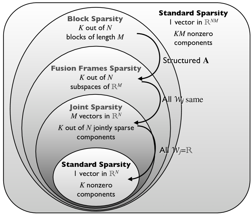
We would also like to note that the hierarchy of such sparsity problems depends on their dimension. For example, a joint sparsity problem with $M=1$ becomes the standard sparsity model. In that sense, joint sparsity models generalize standard sparsity models. The hierarchy of sparsity models is illustrated in the Venn diagram of Fig. 1.

Figure 1: Hierarchy of Sparsity Models

III-F Extensions

Several extensions of this formulation and the work in this paper are possible, but beyond our scope. For example, the analysis we provide is in the exactly sparse, noiseless case. As with classical compressed sensing, it is possible to accommodate sampling in the presence of noise. It is also natural to consider the extension of this work to sampling signals that are not $k$-sparse in a fusion frame representation but can be very well approximated by such a representation. (However, see Section IV-D.)

The richness of fusion frames also allows us to consider richer sampling matrices. Specifically, it is possible to consider sampling operators consisting of different matrices, each operating on a separate subspace of the fusion frame. Such extensions open the use of $\ell_{1}$ methods to general vector-valued mathematical objects, to the general problem of sampling such objects [8], and to general model-based CS problems [28].

IV Deterministic Recovery Conditions

In this section we derive conditions on $\mathbf{c}^{0}$ and $\mathbf{A}$ so that $\mathbf{c}^{0}$ is the unique so lution of ($P_{0}$) as well as of ($P_{1}$). Our approach uses the generalized notions of null space property, coherence and the restricted isometry property, all commonly used measures of morphological difference between the vectors of a measuring matrix.

IV-A Fusion Null Space Property

We first prove Thm. III.4, which demonstrates that the fusion NSP guarantees recovery, similarly to the standard CS setup [20]. This notion will also be useful later to prove recovery bounds using the fusion coherence and using the fusion restricted isometry constants.

Proof:

Assume first that the fusion NSP holds. Let $\mathbf{c}^{0}$ be a vector with $\|\mathbf{c}^{0}\|_{2,0}\leq k$, and let $\mathbf{c}^{1}$ be an arbitrary solution of the system $\mathbf{A}\mathbf{U}(\mathbf{c})=\mathbf{Y}$, and set

$$\mathbf{h}=\mathbf{c}^{1}-\mathbf{c}^{0}.$$

Letting $S$ denote the support of $\mathbf{c}^{0}$, we obtain

$$\|\mathbf{c}^{1}\|_{2,1}-\|\mathbf{c}^{0}\|_{2,1} = \|\mathbf{c}^{1}_{S}\|_{2,1}+\|\mathbf{c}^{1}_{S^{c}}\|_{2,1}-\|\mathbf{c}^{0}_{S}\|_{2,1}$$

$$\geq \|\mathbf{h}_{S^{c}}\|_{2,1}-\|\mathbf{h}_{S}\|_{2,1}.$$

This term is greater than zero for any $\mathbf{h}\neq 0$ provided that

$$\|\mathbf{h}_{S^{c}}\|_{2,1}>\|\mathbf{h}_{S}\|_{2,1}$$ (12)

or, in other words,

$$\tfrac{1}{2}\|\mathbf{h}\|_{2,1}>\|\mathbf{h}_{S}\|_{2,1},$$ (13)

which is ensured by the fusion NSP.

Conversely, assume that all vectors $\mathbf{c}$ with $\|\mathbf{c}\|_{0}\leq k$ are recovered using $(P_{1})$. Then, for any $\mathbf{h}\in{\cal{N}}\setminus\{0\}$ and any $S\subset\{1,\ldots,N\}$ with $|S|\leq k$, the $k$-sparse vector $\mathbf{h}_{S}$ is the unique minimizer of $\|\mathbf{c}\|_{2,1}$ subject to $\mathbf{A}\mathbf{c}=\mathbf{A}\mathbf{h}_{S}$. Further, observe that $\mathbf{A}(-\mathbf{h}_{S^{c}})=\mathbf{A}(\mathbf{h}_{S})$ and $-\mathbf{h}_{S^{c}}\neq\mathbf{h}_{S}$, since $\mathbf{h}\in{\cal{N}}\setminus\{0\}$. Therefore, $\|\mathbf{h}_{S}\|_{2,1}<\|\mathbf{h}_{S^{c}}\|_{2,1}$, which is equivalent to the fusion NSP because $\mathbf{h}$ was arbitrary. ∎

IV-B Fusion Coherence

The fusion coherence is an adaptation of the coherence notion to our more complicated situation involving the angles between the subspaces generated by the bases $\mathbf{U}_{j}$, $j=1,\ldots,N$. In other words, here we face the problem of recovery of vector-valued (instead of scalar-valued) components and our definition is adapted to handle this.

Since the $\mathbf{P}_{j}$’s are projection matrices, we can also rewrite the definition of fusion coherence as

$$\mu_{f}=\max_{j\neq k}\left[|\langle\mathbf{a}_{j},\mathbf{a}_{k}\rangle|\cdot|\lambda_{\max}(\mathbf{P}_{j}\mathbf{P}_{k})|^{1/2}\right]$$

with $\lambda_{\max}$ denoting the largest eigenvalue, simply due to the fact that the eigenvalues of $\mathbf{P}_{k}\mathbf{P}_{j}\mathbf{P}_{k}$ and $\mathbf{P}_{j}\mathbf{P}_{k}$ coincide. Indeed, if $\lambda$ is an eigenvalue of $\mathbf{P}_{j}\mathbf{P}_{k}$ with corresponding eigenvector $v$ then $\mathbf{P}_{k}\mathbf{P}_{j}\mathbf{P}_{k}v=\lambda\mathbf{P}_{k}v$. Since $\mathbf{P}_{k}^{2}=\mathbf{P}_{k}$ this implies that $\mathbf{P}_{k}\mathbf{P}_{j}\mathbf{P}_{k}(\mathbf{P}_{k}v)=\lambda\mathbf{P}_{k}v$ so that $\lambda$ is an eigenvalue of $\mathbf{P}_{k}\mathbf{P}_{j}\mathbf{P}_{k}$ with eigenvector $\mathbf{P}_{k}v$. Let us also remark that $|\lambda_{\max}(\mathbf{P}_{j}\mathbf{P}_{k})|^{1/2}$ equals the largest absolute value of the cosines of the principle angles between $\mathcal{W}_{j}$ and $\mathcal{W}_{k}$.

Before we continue with the proof of the recovery condition in Theorem III.5, let us for a moment consider the following special cases of this theorem.

Case $M=1$

In this case the projection matrices equal $1$, and hence the problem reduces to the classical recovery problem $\mathbf{A}\mathbf{x}=\mathbf{y}$ with $\mathbf{x}\in{\mathbb{R}}^{N}$ and $\mathbf{y}\in{\mathbb{R}}^{n}$. Thus our result reduces to the result obtained in [36], and the fusion coherence coincides with the commonly used mutual coherence, i.e., $\mu_{f}=\max_{j\neq k}|\langle\mathbf{a}_{j},\mathbf{a}_{k}\rangle|$.

Case $\mathcal{W}_{j}={\mathbb{R}}^{M}$ for all $j$

In this case the problem becomes the standard joint sparsity recovery. We recover a matrix $\mathbf{X}^{0}\in{\mathbb{R}}^{N\times M}$ with few non-zero rows from knowledge of $\mathbf{A}\mathbf{X}^{0}\in{\mathbb{R}}^{n\times M}$, without any constraints on the structure of each row of $\mathbf{X}^{0}$. The recovered matrix is the fusion frame representation of the sparse vector and each row $j$ represents a signal in the subspace $\mathcal{W}_{j}$ (the general case has the constraint that $\mathbf{X}^{0}$ is required to be of the form $\mathbf{U}(\mathbf{c}^{0})$). Again fusion coherence coincides with the commonly used mutual coherence, i.e., $\mu_{f}=\max_{j\neq k}|\langle\mathbf{a}_{j},\mathbf{a}_{k}\rangle|$.

Case $\mathcal{W}_{j}\perp\mathcal{W}_{k}$ for all $j,k$

In this case the fusion coherence becomes 0. And this is also the correct answer, since in this case there exists precisely one solution of the system $\mathbf{A}\mathbf{U}(\mathbf{c})=\mathbf{Y}$ for a given $\mathbf{Y}$. Hence Condition (7) becomes meaningless.

General Case

In the general case we can consider two scenarios: either we are given the subspaces $(\mathcal{W}_{j})_{j}$ or we are given the measuring matrix $\mathbf{A}$. In the first situation we face the task of choosing the measuring matrix such that $\mu_{f}$ is as small as possible. Intuitively, we would choose the vectors $(\mathbf{a}_{j})_{j}$ so that a pair $(\mathbf{a}_{j},\mathbf{a}_{k})$ has a large angle if the associated two subspaces $(\mathcal{W}_{j},\mathcal{W}_{k})$ have a small angle, hence balancing the two factors and try to reduce the maximum. In the second situation, we can use a similar strategy now designing the subspaces $(\mathcal{W}_{j})_{j}$ accordingly.

For the proof of Theorem III.5 we first derive a reformulation of the equation $\mathbf{A}\mathbf{U}(\mathbf{c})=\mathbf{Y}$. For this, let $\mathbf{P}_{j}$ denote the orthogonal projection onto $\mathcal{W}_{j}$ for each $j=1,\ldots,N$, set $\mathbf{A}_{\mathbf{P}}$ as in (4) and define the map $\varphi_{k}:{\mathbb{R}}^{k\times M}\to{\mathbb{R}}^{kM}$, $k\geq 1$ by

$$\varphi_{k}(\mathbf{Z})=\varphi_{k}\left(\begin{array}[]{c}\mathbf{z}_{1}\\ \hline\cr\vspace*{-0.5cm}\hfil\\ \vdots\\ \hline\cr\vspace*{-0.45cm}\hfil\\ \mathbf{z}_{k}\end{array}\right)=(\mathbf{z}_{1}\ldots\mathbf{z}_{k})^{T},$$

i.e., the concatenation of the rows. Then it is easy to see that

$$\mathbf{A}\mathbf{U}(\mathbf{c})=\mathbf{Y}\quad\Leftrightarrow\quad\mathbf{A}_{\mathbf{P}}\varphi_{N}(\mathbf{U}(\mathbf{c}))=\varphi_{n}(\mathbf{Y}).$$ (14)

We now split the proof of Theorem III.5 into two lemmas, and wish to remark that many parts are closely inspired by the techniques employed in [36, 31]. We first show that $\mathbf{c}^{0}$ satisfying (7) is the unique solution of $(P_{1})$.

Lemma IV.1

If there exists a solution $\mathbf{U}(\mathbf{c}^{0})\in{\mathbb{R}}^{N\times M}$ of the system $\mathbf{A}\mathbf{U}(\mathbf{c})=\mathbf{Y}$ with $\mathbf{c}^{0}$ satisfying (7), then $\mathbf{c}^{0}$ is the unique solution of $(P_{1})$.

Proof:

We aim at showing that the condition on the fusion coherence implies the fusion NSP. To this end, let $\mathbf{h}\in{\cal{N}}\setminus\{0\}$, i.e., $\mathbf{A}\mathbf{U}(\mathbf{h})=0$. By using the reformulation (14), it follows that

$$\mathbf{A}_{\mathbf{P}}\varphi_{N}(\mathbf{U}(\mathbf{h}))=0.$$

This implies that

$$\mathbf{A}_{\mathbf{P}}^{*}\mathbf{A}_{\mathbf{P}}\varphi_{N}(\mathbf{U}(\mathbf{h}))=0.$$

Defining $\mathbf{a}_{j}$ by $\mathbf{a}_{j}=(a_{ij})_{i}$ for each $j$, the previous equality can be computed to be

$$(\left\langle\mathbf{a}_{j},\mathbf{a}_{k}\right\rangle\mathbf{P}_{j}\mathbf{P}_{k})_{jk}\varphi_{N}(\mathbf{U}(\mathbf{h}))=0.$$

Recall that we have required the vectors $\mathbf{a}_{j}$ to be normalized. Hence, for each $j$,

$$\mathbf{U}_{j}\mathbf{h}_{j}=-\sum_{k\neq j}\left\langle\mathbf{a}_{j},\mathbf{a}_{k}\right\rangle\mathbf{P}_{j}\mathbf{P}_{k}\mathbf{U}_{k}\mathbf{h}_{k}.$$

Since $\|\mathbf{U}_{j}\mathbf{h}_{j}\|_{2}=\|\mathbf{h}_{j}\|_{2}$ for any $j$, this gives

$$\|\mathbf{h}_{j}\|_{2} \leq \sum_{k\neq j}|\langle\mathbf{a}_{j},\mathbf{a}_{k}\rangle|\cdot\|\mathbf{P}_{j}\mathbf{P}_{k}\|_{2\to 2}\|\mathbf{h}_{k}\|_{2}$$

$$\leq \mu_{f}(\|\mathbf{h}\|_{2,1}-\|\mathbf{h}_{j}\|_{2}),$$

which implies

$$\|\mathbf{h}_{j}\|_{2}\leq(1+\mu_{f}^{-1})^{-1}\|\mathbf{h}\|_{2,1}.$$

Thus, we have

$$\|\mathbf{h}_{S}\|_{2,1} \leq \#(S)\cdot(1+\mu_{f}^{-1})^{-1}\|\mathbf{h}\|_{2,1}$$

$$= \|\mathbf{c}^{0}\|_{2,0}\cdot(1+\mu_{f}^{-1})^{-1}\|\mathbf{h}\|_{2,1}.$$

Concluding, (7) and the fusion null space property show that $\mathbf{h}$ satisfies (13) unless $\mathbf{h}=0$, which implies that $\mathbf{c}^{0}$ is the unique minimizer of $(P_{1})$ as claimed. ∎

Using Lemma IV.1 it is easy to show the following lemma.

Lemma IV.2

If there exists a solution $\mathbf{U}(\mathbf{c}^{0})\in{\mathbb{R}}^{N\times M}$ of the system $\mathbf{A}\mathbf{U}(\mathbf{c})=\mathbf{Y}$ with $\mathbf{c}^{0}$ satisfying (7), then $\mathbf{c}^{0}$ is the unique solution of $(P_{0})$.

Proof:

Assume $\mathbf{c}^{0}$ satisfies (7) and $\mathbf{A}\mathbf{U}(\mathbf{c}^{0})=\mathbf{Y}$. Then, by Lemma IV.1, it is the unique solution of $(P_{1})$. Assume there is a $\tilde{\mathbf{c}}$ satisfying $\mathbf{A}\mathbf{U}(\tilde{\mathbf{c}})=\mathbf{Y}$ such that $\|\tilde{\mathbf{c}}\|_{2,0}\leq\|\mathbf{c}^{0}\|_{2,0}$. Then $\tilde{\mathbf{c}}$ also satisfies (7) and again by Lemma IV.1 $\tilde{\mathbf{c}}$ is also the unique solution to $(P_{1})$. But this means that $\tilde{\mathbf{c}}=\mathbf{c}^{0}$ and $\mathbf{c}^{0}$ is the unique solution to $(P_{0})$. ∎

We observe that Theorem III.5 now follows immediately from Lemmas IV.1 and IV.2.

IV-C Fusion Restricted Isometry Property

Finally, we consider the condition for sparse recovery using the restricted isometry property (RIP) of the sampling matrix. The RIP property on the sampling matrix, first introduced in [1], complements the null space propery and the mutual coherence conditions. Definition III.3 generalizes it for the fusion frame setup. Informally, we say that $(\mathbf{A},(\mathcal{W}_{j})_{j=1}^{N})$ satisfies the fusion restricted isometry property (FRIP) if $\delta_{k}$ is small for reasonably large $k$. Note that we obtain the classical definition of the RIP of $\mathbf{A}$ if $M=1$ and all the subspaces $\mathcal{W}_{j}$ have dimension $1$. Using this property we can prove Theorem III.6.

Proof:

The proof proceeds analogously to the one of Theorem 2.6 in [26], that is, we establish the fusion NSP. The claim will then follow from Theorem III.4.

Let us first note that

$$|\langle\mathbf{A}_{\mathbf{P}}\mathbf{u},\mathbf{A}_{\mathbf{P}}\mathbf{v}\rangle|\leq\delta_{k}\|\mathbf{u}\|_{2,2}\|\mathbf{v}\|_{2,2}$$

for all $\mathbf{u}=(\mathbf{u}_{1},\ldots,\mathbf{u}_{N}),\mathbf{v}=(\mathbf{v}_{1},\ldots,\mathbf{v}_{N})\in{\mathbb{R}}^{MN}$, $\mathbf{u}_{j},\mathbf{v}_{j}\in{\mathbb{R}}^{M}$, with ${\text{\rm supp}}\,\mathbf{u}=\{j:\mathbf{u}_{j}\neq 0\}\cap{\text{\rm supp}}\,\mathbf{v}=\emptyset$ and $\|\mathbf{u}\|_{2,0}+\|\mathbf{v}\|_{2,0}\leq k$. This statement follows completely analogously to the proof of Proposition 2.5(c) in [32], see also [37, 20].

Now let $\mathbf{h}\in{\cal{N}}=\{\mathbf{h}:\mathbf{A}\mathbf{U}(\mathbf{h})=0\}$ be given. Using the reformulation (14), it follows that

$$\mathbf{A}_{\mathbf{P}}\varphi_{N}(\mathbf{U}(\mathbf{h}))=0.$$

In order to show the fusion NSP it is enough to consider an index set $S_{0}$ of size $k$ of largest components $\|\mathbf{h}_{j}\|_{2}$, i.e., $\|\mathbf{h}_{j}\|_{2}\geq\|\mathbf{h}_{i}\|_{2}$ for all $j\in S_{0}$, $i\in S_{0}^{c}=\{1,\ldots,N\}\setminus S_{0}$. We partition $S_{0}^{c}$ into index sets $S_{1},S_{2},\ldots$ of size $k$ (except possibly the last one), such that $S_{1}$ is an index set of largest components in $S_{0}^{c}$, $S_{2}$ is an index set of largest components in $(S_{0}\cup S_{0})^{c}$, etc. Let $\mathbf{h}_{S_{i}}$ be the vector that coincides with $\mathbf{h}$ on $S_{i}$ and is set to zero outside. In view of $\mathbf{h}\in{\cal{N}}$ we have $\mathbf{A}\mathbf{U}(\mathbf{h}_{S_{0}})=\mathbf{A}\mathbf{U}(-\mathbf{h}_{S_{1}}-\mathbf{h}_{S_{2}}-\cdots)$. Now set $\mathbf{z}=\varphi_{N}(\mathbf{U}(\mathbf{h}))$ and $\mathbf{z}_{S_{i}}=\varphi_{N}(\mathbf{U}(\mathbf{h}_{S_{i}}))$. It follows that $\mathbf{A}_{\mathbf{P}}(\mathbf{z}_{S_{0}})=\mathbf{A}_{\mathbf{P}}(-\sum_{i\geq 1}\mathbf{z}_{S_{i}})$. By definition of the FRIP we obtain

$$\|\mathbf{h}_{S_{0}}\|_{2,2}^{2} = \|\mathbf{z}_{S_{0}}\|_{2,2}^{2}\leq\frac{1}{1-\delta_{k}}\|\mathbf{A}_{\mathbf{P}}\mathbf{z}_{S_{0}}\|_{2,2}^{2}$$

$$= \frac{1}{1-\delta_{k}}\Big{\langle}\mathbf{A}_{\mathbf{P}}\mathbf{z}_{S_{0}},\mathbf{A}_{\mathbf{P}}\big{(}-\sum_{i\geq 1}\mathbf{z}_{S_{i}}\big{)}\Big{\rangle}$$

$$\leq \frac{1}{1-\delta_{k}}\sum_{i\geq 1}|\langle\mathbf{A}_{\mathbf{P}}\mathbf{z}_{S_{0}},\mathbf{A}_{\mathbf{P}}(-\mathbf{z}_{S_{i}})\rangle|$$

$$\leq \frac{\delta_{2k}}{1-\delta_{k}}\|\mathbf{z}_{S_{0}}\|_{2,2}\cdot\sum_{i\geq 1}\|\mathbf{z}_{S_{i}}\|_{2,2}.$$

Using that $\delta_{k}\leq\delta_{2k}$ and dividing by $\|\mathbf{z}_{S_{0}}\|_{2,2}$ yields

$$\|\mathbf{z}_{S_{0}}\|_{2,2}\leq\frac{\delta_{2k}}{1-\delta_{2k}}\sum_{i\geq 1}\|\mathbf{z}_{S_{i}}\|_{2,2}.$$

By construction of the sets $S_{i}$ we have $\|\mathbf{z}_{j}\|_{2}\leq\frac{1}{k}\sum_{\ell\in S_{i-1}}\|\mathbf{z}_{\ell}\|_{2}$ for all $j\in S_{i}$, hence,

$$\|\mathbf{z}_{S_{i}}\|_{2,2}=\big{(}\sum_{j\in S_{i}}\|\mathbf{z}_{j}\|_{2}^{2}\big{)}^{1/2}\leq\frac{1}{\sqrt{k}}\|\mathbf{z}_{S_{i-1}}\|_{2,1}.$$

The Cauchy-Schwarz inequality yields

$$\|\mathbf{h}_{S_{0}}\|_{2,1} \leq \sqrt{k}\|\mathbf{h}_{S_{0}}\|_{2,2}\leq\frac{\delta_{2k}}{1-\delta_{2k}}\sum_{i\geq 1}\|\mathbf{z}_{S_{i-1}}\|_{2,1}$$

$$\leq \frac{\delta_{2k}}{1-\delta_{2k}}(\|\mathbf{z}_{S_{0}}\|_{2,1}+\|\mathbf{z}_{S_{0}^{c}}\|_{2,1})<\frac{1}{2}\|\mathbf{h}\|_{2,1},$$

where we used the assumption $\delta_{2k}<1/3$. Hence, the fusion null space property follows. ∎

Having proved that the FRIP ensures signal recovery, our next proposition relates the classical RIP with our newly introduced FRIP. Let us note, however, that using the RIP to guarantee the FRIP does not take into account any properties of the fusion frame, so it is sub-optimal—especially if the subspaces of the fusion frame are orthogonal or almost orthogonal.

Proposition IV.3

Let $\mathbf{A}\in{\mathbb{R}}^{n\times N}$ with classical restricted isometry constant $\tilde{\delta}_{k}$, that is,

$$(1-\tilde{\delta}_{k})\|y\|_{2}^{2}\leq\|\mathbf{A}y\|_{2}^{2}\leq(1+\tilde{\delta}_{k})\|y\|_{2}^{2}$$

for all $k$-sparse $y\in{\mathbb{R}}^{N}$. Let $(\mathcal{W}_{j})_{j=1}^{N}$ be an arbitrary fusion frame for ${\mathbb{R}}^{M}$. Then the fusion restricted isometry constant $\delta_{k}$ of $(\mathbf{A},(\mathcal{W})_{j=1}^{N})$ satisfies $\delta_{k}\leq\tilde{\delta}_{k}$.

Proof:

Let $\mathbf{c}$ satisfy $\|\mathbf{c}\|_{0}\leq k$, and denote the columns of the matrix $\mathbf{U}(\mathbf{c})$ by $\mathbf{u}_{1},\ldots,\mathbf{u}_{M}$. The condition $\|\mathbf{c}\|_{0}\leq k$ implies that each $\mathbf{u}_{i}$ is $k$-sparse. Since $\mathbf{A}$ satisfies the RIP of order $k$ with constant $\delta_{k}$, we obtain

$$\|\mathbf{A}\mathbf{U}(\mathbf{c})\|_{2,2}^{2} = \sum_{i=1}^{M}\|\mathbf{A}\mathbf{u}_{i}\|_{2}^{2}\leq(1+\delta_{k})\sum_{i=1}^{M}\|\mathbf{u}_{i}\|_{2}^{2}$$

$$= (1+\delta_{k})\|\mathbf{U}(\mathbf{c})\|_{2,2}^{2}=(1+\delta_{k})\|\mathbf{c}\|_{2,2}^{2}$$

as well as

$$\|\mathbf{A}\mathbf{U}(\mathbf{c})\|_{2,2}^{2} = \sum_{i=1}^{M}\|\mathbf{A}\mathbf{u}_{i}\|_{2}^{2}\geq(1-\delta_{k})\sum_{i=1}^{M}\|\mathbf{u}_{i}\|_{2}^{2}$$

$$= (1-\delta_{k})\|\mathbf{U}(\mathbf{c})\|_{2,2}^{2}=(1-\delta_{k})\|\mathbf{c}\|_{2,2}^{2}.$$

This proves the proposition because $\mathbf{A}\mathbf{U}(\mathbf{c})=\mathbf{A}_{\mathbf{P}}\mathbf{U}(\mathbf{c})$. ∎

IV-D Additional Remarks and Extensions

Of course, it is possible to extend the proof of Theorem III.6 in a similar manner to [1, 37, 38, 39] such that we can accommodate measurement noise and signals that are well approximated by sparse fusion frame representation. We state the analog of the main theorem of [37] without proof.

Theorem IV.4

Assume that the fusion restricted isometry constant $\delta_{2k}$ of $(\mathbf{A},(\mathcal{W}_{j})_{j=1}^{N})$ satisfies

$$\delta_{2k}<\Delta:=\sqrt{2}-1\approx 0.4142.$$

For $\mathbf{x}\in\mathcal{H}$, let noisy measurements $\mathbf{Y}=\mathbf{A}\mathbf{x}+\eta$ be given with $\|\eta\|_{2}\leq\epsilon$. Let $\mathbf{c}^{\#}$ be the solution of the convex optimization problem

$$\min\|\mathbf{c}\|_{2,1}\quad\mbox{subject to}\quad\|\mathbf{A}\mathbf{U}(\mathbf{c})-\mathbf{Y}\|_{2,2}\leq\eta,$$

and set $\mathbf{x}^{\#}=\mathbf{U}(\mathbf{c}^{\#})$. Then

$$\|\mathbf{x}-\mathbf{x}^{\#}\|_{2,2}\leq C_{1}\eta+C_{2}\frac{\|\mathbf{x}^{k}-\mathbf{x}\|_{2,1}}{\sqrt{k}}$$

where $\mathbf{x}_{k}$ is obtained from $\mathbf{x}$ be setting to zero all components except the $k$ largest in norm. The constants $C_{1},C_{2}>0$ only depend on $\delta_{2k}$ (or rather on $\Delta-\delta_{2k}$).

V Probabilistic Analysis

V-A General Recovery Condition

We start our analysis by deriving a recovery condition on the measurement matrix and the signal which the reader might want to compare with [40, 41]. Given a matrix $\mathbf{X}\in{\mathbb{R}}^{N\times M}$, we let ${\rm sgn}(\mathbf{X})\in{\mathbb{R}}^{N\times M}$ denote the matrix which is generated from $\mathbf{X}$ by normalizing each entry $X_{ji}$ by the norm of the corresponding row $\mathbf{X}_{j,\cdot}$. More precisely,

$${\rm sgn}(\mathbf{X})_{ji}=\left\{\begin{array}[]{ccl}\frac{X_{ji}}{\|\mathbf{X}_{j,\cdot}\|_{2}}&\mbox{~{}if~{}}&\|\mathbf{X}_{j,\cdot}\|_{2}\neq 0,\\ 0&\mbox{~{}if~{}}&\|\mathbf{X}_{j,\cdot}\|_{2}=0.\end{array}\right.$$

Column vectors are defined similarly by $\mathbf{X}_{\cdot,i}$.

Under a certain condition on $A$, which is dependent on the support of the solution, we derive the result below on unique recovery. To phrase it, let $(\mathcal{W}_{j})_{j=1}^{N}$ be a fusion frame with associated orthogonal bases $(\mathbf{U}_{j})_{j=1}^{N}$ and orthogonal projections $(\mathbf{P}_{j})_{j=1}^{N}$, and recall the definition of the notion $\mathbf{U}(\mathbf{c})$ in Section III. Then, for some support set $S=\{j_{1},\ldots,j_{|S|}\}\subseteq\{1,\ldots,N\}$ of $\mathbf{U}(\mathbf{c})$, we let

$$\mathbf{A}_{S}=(\mathbf{A}_{\cdot,j_{1}}\cdots\mathbf{A}_{\cdot,j_{|S|}})\in{\mathbb{R}}^{n\times|S|}$$

and

$$\mathbf{U}(\mathbf{c})_{S}=\left(\begin{array}[]{c}\mathbf{c}_{j_{1}}^{T}\mathbf{U}_{j_{1}}^{T}\\ \hline\cr\vspace*{-0.5cm}\hfil\\ \vdots\\ \hline\cr\vspace*{-0.45cm}\hfil\\ \mathbf{c}_{j_{|S|}}^{T}\mathbf{U}_{j_{|S|}}^{T}\end{array}\right)\in{\mathbb{R}}^{|S|\times M}.$$

Before stating the theorem, we wish to remark that its proof uses similar ideas as the analog proof in [7]. We however state all details for the convenience of the reader.

Theorem V.1

Retaining the notions from the beginning of this section, we let $\mathbf{c}_{j}\in{\mathbb{R}}^{m_{j}}$, $j=1\ldots,N$ with $S={\text{\rm supp}}(\mathbf{c})=\{j:\mathbf{c}_{j}\neq 0\}$. If $\mathbf{A}_{S}$ is non-singular and there exists a matrix $\mathbf{H}\in{\mathbb{R}}^{n\times M}$ such that

$$\mathbf{A}_{S}^{T}\mathbf{H}={\rm sgn}(\mathbf{U}(\mathbf{c})_{S})$$ (15)

and

$$\|\mathbf{H}^{T}\mathbf{A}_{\cdot,j}\|_{2}<1\quad\mbox{for all }j\not\in S,$$ (16)

then $\mathbf{U}(\mathbf{c})$ is the unique solution of $(P_{1})$.

Proof:

Let $\mathbf{c}_{j}\in{\mathbb{R}}^{m_{j}}$, $j=1\ldots,N$ be a solution of $\mathbf{Y}=\mathbf{A}\mathbf{U}(\mathbf{c})$, set $S={\text{\rm supp}}(\mathbf{U}(\mathbf{c}))$, and suppose $\mathbf{A}_{S}$ is non-singular and the hypotheses (15) and (16) are satisfied for some matrix $\mathbf{H}\in{\mathbb{R}}^{n\times M}$. Let $\mathbf{c}^{\prime}_{j}\in{\mathbb{R}}^{m_{j}}$, $j=1\ldots,N$ with $\mathbf{c}^{\prime}_{j_{0}}\neq\mathbf{c}_{j_{0}}$ for some $j_{0}$ be a different set of coefficient vectors which satisfies $\mathbf{Y}=\mathbf{A}\mathbf{U}(\mathbf{c}^{\prime})$. To prove our result we aim to establish that

$$\|\mathbf{c}\|_{2,1}<\|\mathbf{c}^{\prime}\|_{2,1}.$$ (17)

We first observe that

$$\|\mathbf{c}\|_{2,1} = \|\mathbf{U}(\mathbf{c})\|_{2,1}=\|\mathbf{U}(\mathbf{c})_{S}\|_{2,1}$$

$$= \textnormal{tr}\left[{\rm sgn}(\mathbf{U}(\mathbf{c})_{S})(\mathbf{U}(\mathbf{c})_{S})^{T}\right].$$

Set $S^{\prime}={\text{\rm supp}}(\mathbf{U}(\mathbf{c}^{\prime}))$, apply (15), and exploit properties of the trace,

$$\|\mathbf{c}\|_{2,1} = \textnormal{tr}\left[\mathbf{A}_{S}^{T}\mathbf{H}(\mathbf{U}(\mathbf{c})_{S})^{T}\right]=\textnormal{tr}\left[(\mathbf{A}\mathbf{U}(\mathbf{c}))^{T}\mathbf{H}\right]$$

$$= \textnormal{tr}\left[(\mathbf{A}\mathbf{U}(\mathbf{c}^{\prime}))^{T}\mathbf{H}\right]$$

$$= \textnormal{tr}\left[(\mathbf{A}\mathbf{U}(\mathbf{c}^{\prime}_{S}))^{T}\mathbf{H}\right]+\textnormal{tr}\left[(\mathbf{A}\mathbf{U}(\mathbf{c}^{\prime}_{S^{c}}))^{T}\mathbf{H}\right].$$

Now use the Cauchy-Schwarz inequality to obtain

$$\|\mathbf{c}\|_{2,1} \leq \sum_{j\in S}\|(\mathbf{U}(\mathbf{c}^{\prime})_{S})_{j,\cdot}\|_{2}\|(\mathbf{H}^{T}\mathbf{A}_{S})_{\cdot,j}\|_{2}$$

$$+ \sum_{j\in S^{c}}\|(\mathbf{U}(\mathbf{c}^{\prime})_{S^{c}})_{j,\cdot}\|_{2}\|(\mathbf{H}^{T}\mathbf{A}_{S^{c}})_{\cdot,j}\|_{2}$$

$$\leq \max_{j\in S}\|(\mathbf{H}^{T}\mathbf{A}_{S})_{\cdot,j}\|_{2}\|\mathbf{c}^{\prime}_{S}\|_{2,1}$$

$$+ \max_{j\in S^{c}}\|(\mathbf{H}^{T}\mathbf{A}_{S^{c}})_{\cdot,j}\|_{2}\|\mathbf{c}^{\prime}_{S^{c}}\|_{2,1}$$

$$< \|\mathbf{c}^{\prime}_{S}\|_{2,1}+\|\mathbf{c}^{\prime}_{S^{c}}\|_{2,1}=\|\mathbf{c}^{\prime}\|_{2,1}.$$

The strict inequality follows from $\|\mathbf{c}^{\prime}_{S^{c}}\|_{1}>0$, which is true because otherwise $\mathbf{c}^{\prime}$ would be supported on $S$. The equality $\mathbf{A}\mathbf{U}(\mathbf{c})=\mathbf{A}\mathbf{U}(\mathbf{c}^{\prime})$ would then be in contradiction to the injectivity of $\mathbf{A}_{S}$ (recall that $\mathbf{c}\neq\mathbf{c}^{\prime}$). This concludes the proof. ∎

The matrix $\mathbf{H}$ exploited in Theorem V.1 might be chosen as

$$\mathbf{H}=(\mathbf{A}_{S}^{\dagger})^{T}{\rm sgn}(\mathbf{U}(\mathbf{c})_{S})$$

to satisfy (15). This particular choice will in fact be instrumental for the average case result we are aiming for. For now, we obtain the following result as a corollary from Theorem V.1.

Corollary V.2

Retaining the notions from the beginning of this section, we let $\mathbf{c}_{j}\in{\mathbb{R}}^{m_{j}}$, $j=1\ldots,N$, with $S={\text{\rm supp}}(\mathbf{U}(\mathbf{c}))$. If $\mathbf{A}_{S}$ is non-singular and

$$\|{\rm sgn}(\mathbf{U}(\mathbf{c})_{S})^{T}\mathbf{A}_{S}^{\dagger}\mathbf{A}_{\cdot,j}\|_{2}<1\quad\mbox{for all }j\not\in S,$$ (18)

then $\mathbf{U}(\mathbf{c})$ is the unique solution of $(P_{1})$.

For later use, we will introduce the matrices $\tilde{\mathbf{U}}_{j}\in{\mathbb{R}}^{M\times Nm}$ defined by

$$\tilde{\mathbf{U}}_{j}=({\bf 0}_{M\times m}|\cdots|{\bf 0}_{M\times m}|\mathbf{U}_{j}|{\bf 0}_{M\times m}|\cdots|{\bf 0}_{M\times m}),$$

where $\mathbf{U}_{j}$ is the $j$th block. For some $\mathbf{b}=(b_{1},\ldots,b_{k})^{T}\in{\mathbb{R}}^{k}$, we can then write $\mathbf{U}(\mathbf{c})_{S}^{T}\mathbf{b}$ as

$$\sum_{\ell=1}^{k}b_{\ell}\tilde{\mathbf{U}}_{j_{\ell}}\mathbf{X}\in{\mathbb{R}}^{M}.$$ (19)

Using the above and the probabilistic model in Sec. III-D to prove our main probabilistic result, Theorem III.7.

V-B Probability of Sparse Recovery for Fusion Frames

The proof of our probabilistic result, Theorem III.7, is developed in several steps. A key ingredient is a concentration of measure result: If $f$ is a Lipschitz function on ${\mathbb{R}}^{K}$ with Lipschitz constant $L$, i.e., $|f(x)-f(y)|\leq L\|x-y\|_{2}$ for all $x,y\in{\mathbb{R}}^{K}$, $\mathbf{X}$ is a $K$-dimensional vector of independent standard normal random variables then [42, eq. (2.35)]

$${\mathbb{P}}(|f(X)-{\mathbb{E}}f(X)|\geq u)\leq 2e^{-u^{2}/(2L^{2})}\quad\mbox{ for all }u>0.$$ (20)

Our first lemma investigates the properties of a function related to (19) that are needed to apply the above inequality.

Lemma V.3

Let $\mathbf{b}=(b_{1},\ldots,b_{k})^{T}\in{\mathbb{R}}^{k}$ and $S=\{j_{1},\ldots,j_{k}\}\subseteq\{1,\ldots,N\}$. Define the function $f$ by

$$f(\mathbf{X})=\|\sum_{\ell=1}^{k}b_{\ell}\tilde{\mathbf{U}}_{j_{\ell}}\mathbf{X}\|_{2},\quad\mathbf{X}\in{\mathbb{R}}^{Nm}.$$

Then the following holds.

• $f$ is Lipschitz with constant $\|\sum_{\ell=1}^{k}b_{\ell}\tilde{\mathbf{U}}_{j_{\ell}}\|_{2\to 2}$.

• For a standard Gaussian vector $\mathbf{X}\in{\mathbb{R}}^{Nm}$ we have $\mathbb{E}[f(\mathbf{X})]\leq\sqrt{m}\|\mathbf{b}\|_{2}$.

Proof:

The claim in (i) follows immediately from

$$|f(\mathbf{X})-f(\mathbf{Y})| = \Big{|}\|\sum_{\ell=1}^{k}b_{\ell}\tilde{\mathbf{U}}_{j_{\ell}}\mathbf{X}\|_{2}-\|\sum_{\ell=1}^{k}b_{\ell}\tilde{\mathbf{U}}_{j_{\ell}}\mathbf{Y}\|_{2}\Big{|}$$

$$\leq \|\left(\sum_{\ell=1}^{k}b_{\ell}\tilde{\mathbf{U}}_{j_{\ell}}\right)(\mathbf{X}-\mathbf{Y})\|_{2}$$

$$\leq \|\sum_{\ell=1}^{k}b_{\ell}\tilde{\mathbf{U}}_{j_{\ell}}\|_{2\to 2}\|\mathbf{X}-\mathbf{Y}\|_{2}.$$

It remains to prove (ii). Obviously,

$$\left(\mathbb{E}f(\mathbf{X})\right)^{2} \leq \mathbb{E}[f(\mathbf{X})^{2}]=\mathbb{E}\left[\sum_{i=1}^{M}\Big{|}\sum_{\ell=1}^{k}b_{\ell}(\tilde{\mathbf{U}}_{j_{\ell}}\mathbf{X})_{i}\Big{|}^{2}\right]$$

$$= \sum_{i=1}^{M}\sum_{\ell,\ell^{\prime}=1}^{k}b_{\ell}b_{\ell^{\prime}}\mathbb{E}[(\tilde{\mathbf{U}}_{j_{\ell}}\mathbf{X})_{i}(\tilde{\mathbf{U}}_{j_{\ell^{\prime}}}\mathbf{X})_{i}].$$

Invoking the conditions on $\mathbf{X}$,

$$\mathbb{E}[f(\mathbf{X})]^{2} \leq \sum_{i=1}^{M}\sum_{\ell=1}^{k}b_{\ell}^{2}\mathbb{E}[(\tilde{\mathbf{U}}_{j_{\ell}}\mathbf{X})_{i}]^{2}=\sum_{\ell=1}^{k}b_{\ell}^{2}\|\tilde{\mathbf{U}}_{j_{\ell}}\|_{F}^{2}$$

$$= m\|\mathbf{b}\|_{2}^{2}.$$

∎

Next we estimate the Lipschitz constant of the function $f$ in the previous lemma.

Lemma V.4

Let $\mathbf{b}=(b_{1},\ldots,b_{k})^{T}\in{\mathbb{R}}^{k}$ and $S=\{j_{1},\ldots,j_{k}\}\subseteq\{1,\ldots,N\}$. Then

$$\|\sum_{\ell=1}^{k}b_{\ell}\tilde{\mathbf{U}}_{j_{\ell}}\|_{2\to 2}\leq\|\mathbf{b}\|_{\infty}\sqrt{1+\max_{i\in S}\sum_{j\in S,j\neq i}\lambda_{\max{}}(\mathbf{P}_{i}\mathbf{P}_{j})^{1/2}}.$$

Proof:

First observe that

$$\|\sum_{\ell=1}^{k}b_{\ell}\tilde{\mathbf{U}}_{j_{\ell}}\|_{2\to 2} = \|(\sum_{\ell=1}^{k}b_{\ell}\tilde{\mathbf{U}}_{j_{\ell}})^{T}(\sum_{\ell=1}^{k}b_{\ell}\tilde{\mathbf{U}}_{j_{\ell}})\|_{2\to 2}^{1/2}$$

$$= \|\sum_{\ell,\ell^{\prime}=1}^{k}b_{\ell}b_{\ell^{\prime}}\tilde{\mathbf{U}}_{j_{\ell}}^{T}\tilde{\mathbf{U}}_{j_{\ell^{\prime}}}\|_{2\to 2}^{1/2}.$$

Since

$$\|\sum_{\ell,\ell^{\prime}=1}^{k}b_{\ell}b_{\ell^{\prime}}\tilde{\mathbf{U}}_{j_{\ell}}^{T}\tilde{\mathbf{U}}_{j_{\ell^{\prime}}}\|_{2\to 2}\leq\|\mathbf{b}\|_{\infty}^{2}\|(\mathbf{U}_{i}^{T}\mathbf{U}_{j})_{i,j\in S}\|_{2\to 2},$$

it follows that

$$\|\sum_{\ell=1}^{k}b_{\ell}\tilde{\mathbf{U}}_{j_{\ell}}\|_{2\to 2}\leq\|\mathbf{b}\|_{\infty}\|(\mathbf{U}_{i}^{T}\mathbf{U}_{j})_{i,j\in S}\|_{2\to 2}^{1/2}.$$ (21)

Next,

$$\|(\mathbf{U}_{i}^{T}\mathbf{U}_{j})_{i,j\in S}\|_{2\to 2}\leq\max_{i\in S}\sum_{j\in S}\|\mathbf{U}_{i}^{T}\mathbf{U}_{j}\|_{2\to 2}$$

$$= 1+\max_{i\in S}\sum_{j\in S,j\neq i}\|\mathbf{U}_{i}^{T}\mathbf{U}_{j}\|_{2\to 2}.$$

By definition of the orthogonal projections $\mathbf{P}_{i}$,

$$\|\mathbf{U}_{i}^{T}\mathbf{U}_{j}\|_{2\to 2} = \|(\mathbf{U}_{i}^{T}\mathbf{U}_{j})^{T}\mathbf{U}_{i}^{T}\mathbf{U}_{j}\|_{2\to 2}^{1/2}$$

$$= \|\mathbf{U}_{i}^{T}\mathbf{U}_{j}\mathbf{U}_{j}^{T}\mathbf{U}_{i}\|_{2\to 2}^{1/2}=\|\mathbf{P}_{i}\mathbf{P}_{j}\|_{2\to 2}^{1/2}$$

$$= \lambda_{\max{}}(\mathbf{P}_{i}\mathbf{P}_{j})^{1/2}.$$

Combining with (V-B),

$$\|(\mathbf{U}_{i}^{T}\mathbf{U}_{j})_{i,j\in S}\|_{2\to 2}\leq 1+\max_{i\in S}\sum_{j\in S,j\neq i}\lambda_{\max{}}(\mathbf{P}_{i}\mathbf{P}_{j})^{1/2}.$$ (23)

The lemma now follows from (21), (V-B), and (23). ∎

Now we have collected all ingredients to prove our main result, Theorem III.7

Proof:

Denote $\mathbf{b}^{(j)}=(b_{1}^{(j)},\ldots,b_{k}^{(j)})^{T}=\mathbf{A}_{S}^{\dagger}\mathbf{A}_{\cdot,j}\in{\mathbb{R}}^{k}$ for all $j\not\in S$ and choose $\delta\in(0,1-\alpha^{2})$. By Corollary V.2, the probability that the minimization problem ($P_{1}$) fails to recover $\mathbf{U}(\mathbf{c})$ from $\mathbf{Y}=\mathbf{A}\mathbf{U}(\mathbf{c})$ can be estimated as

$${\mathbb{P}}\left(\max_{j\notin S}\|{\rm sgn}(\mathbf{U}(\mathbf{c})_{S})^{T}\mathbf{b}^{(j)}\|_{2}>1\right)$$

$$= {\mathbb{P}}\left(\max_{j\not\in S}\|\sum_{\ell=1}^{k}b_{\ell}^{(j)}\|U_{j_{\ell}}\mathbf{X}_{\ell}\|_{2}^{-1}\tilde{\mathbf{U}}_{j_{\ell}}\mathbf{X}\|_{2}>1\right)$$

$$\leq {\mathbb{P}}\left(\max_{j\not\in S}\|\sum_{\ell=1}^{k}b_{\ell}^{(j)}\tilde{\mathbf{U}}_{j_{\ell}}\mathbf{X}\|_{2}>\sqrt{(1-\delta)m}\right)$$

$$+ {\mathbb{P}}\left(\max_{\ell=1,\ldots,k}\|U_{j_{\ell}}\mathbf{X}_{\ell}\|_{2}<\sqrt{(1-\delta)m}\right)$$

$$\leq \sum_{j\notin S}{\mathbb{P}}\left(\|\sum_{\ell=1}^{k}b_{\ell}^{(j)}\tilde{\mathbf{U}}_{j_{\ell}}\mathbf{X}\|_{2}>\sqrt{(1-\delta)m}\right)$$

$$+ \sum_{\ell=1}^{k}{\mathbb{P}}\left(\|\mathbf{X}_{\ell}\|_{2}^{2}\leq(1-\delta)m\right).$$

Since $\mathbf{X}_{\ell}$ is a standard Gaussian vector in ${\mathbb{R}}^{m}$ [43, Corollary 3] gives

$${\mathbb{P}}\left(\|\mathbf{X}_{\ell}\|_{2}^{2}\leq(1-\delta)m\right)\leq\exp(-\delta^{2}m/4).$$

Furthermore, the concentration inequality (20) combined with Lemmas V.3 and Lemma V.4 yields

$${\mathbb{P}}\left(\|\sum_{\ell=1}^{k}b_{\ell}^{(j)}\tilde{\mathbf{U}}_{j_{\ell}}\mathbf{X}\|_{2}>\sqrt{(1-\delta)m}\right)$$

$$= {\mathbb{P}}\left(\|\sum_{\ell=1}^{k}b_{\ell}^{(j)}\tilde{\mathbf{U}}_{j_{\ell}}\mathbf{X}\|_{2}>\|b^{(j)}\|_{2}\sqrt{m}\right.$$

$$\phantom{{\mathbb{P}}\left(\sum_{j}^{n}\right)}\left.+(\sqrt{1-\delta}-\|b^{(j)}\|_{2})\sqrt{m}\right)$$

$$\leq \exp\left(-\frac{(\sqrt{1-\delta}-\|b^{(j)}\|_{2})^{2}m}{2\|b^{(j)}\|_{\infty}^{2}\theta}\right)$$

$$\leq \exp\left(-\frac{(\sqrt{1-\delta}-\|b^{(j)}\|_{2})^{2}m}{2\|b^{(j)}\|_{2}^{2}\theta}\right)$$

$$\leq \exp\left(-\frac{(\sqrt{1-\delta}-\alpha)^{2}m}{2\alpha^{2}\theta}\right).$$

Combining the above estimates yields the statement of the Theorem. ∎

VI Conclusions and Discussion

The main contribution in this paper is the generalization of standard Compressed Sensing results for sparse signals to signals that have a sparse fusion frame representation. As we demonstrated, the results generalize to fusion frames in a very nice and easy to apply way, using the mixed $\ell_{2}/\ell_{1}$ norm.

A key result in our work shows that the structure in fusion frames provides additional information that can be exploited in the measurement process. Specifically, our definition of fusion coherence demonstrates the importance of prior knowledge about the signal structure. Indeed, if we know that the signal lies in subspaces with very little overlap (i.e., where $\|\mathbf{P}_{j}\mathbf{P}_{k}\|_{2}$ is small in Definition III.2) we can relax the requirement on the coherence of the corresponding vectors in the sampling matrix (i.e., $|\langle\mathbf{a}_{j},\mathbf{a}_{k}\rangle|$ in the same definition) and maintain a low fusion coherence. This behavior emerges from the inherent structure of fusion frames.

The emergence of this behavior is evident both in the guarantees provided by the fusion coherence, and in our average case analysis. Unfortunately, our analysis of this property currently has not been incorporated in a tight approach to satisfying the Fusion RIP property, as described in Section IV-C. While an extension of such analysis for the RIP guarantees is desirable, it is still an open problem.

Our average case analysis also demonstrates that as the sparsity structure of the problem becomes more intricate, the worst case analysis can become too pessimistic for many practical cases. The average case analysis provides reassurance that typical behavior is as expected; significantly better compared to the worst case. Our results corroborate and extend similar findings for the special case of joint sparsity in [7].

Petros T. Boufounos completed his undergraduate and graduate studies at MIT. He received the S.B. degree in Economics in 2000, the S.B. and M.Eng. degrees in Electrical Engineering and Computer Science (EECS) in 2002, and the Sc.D. degree in EECS in 2006. Since January 2009 he is with Mitsubishi Electric Research Laboratories (MERL) in Cambridge, MA. He is also a visiting scholar at the Rice University Electrical and Computer Engineering department. Between September 2006 and December 2008, Dr. Boufounos was a postdoctoral associate with the Digital Signal Processing Group at Rice University doing research in Compressive Sensing. In addition to Compressive Sensing, his immediate research interests include signal acquisition and processing, data representations, frame theory, and machine learning applied to signal processing. He is also looking into how Compressed Sensing interacts with other fields that use sensing extensively, such as robotics and mechatronics. Dr. Boufounos has received the Ernst A. Guillemin Master Thesis Award for his work on DNA sequencing and the Harold E. Hazen Award for Teaching Excellence, both from the MIT EECS department. He has also been an MIT Presidential Fellow. Dr. Boufounos is a member of the IEEE, Sigma Xi, Eta Kappa Nu, and Phi Beta Kappa.

Gitta Kutyniok received diploma degrees in mathematics and computer science in 1996 and the Dr. rer. nat. in mathematics in 2000 from the University of Paderborn. In 2001, she spent one term as a Visiting Assistant Professor at the Georgia Institute of Technology. She then held positions as a Scientific Assistant at the University of Paderborn and the University of Gießen. From Oct. 2004 to Sept. 2005, she was funded by a Research Fellowship by the DFG-German Research Foundation and spent six months at each Washington University in St. Louis and Georgia Institute of Technology. She completed her Habilitation in mathematics in 2006 and received her venia legendi. In 2006, she was awarded a Heisenberg Fellowship by the DFG. From Apr. 2007 to Sept. 2008, she was a Visiting Fellow at Princeton University, Stanford University, and Yale University. Since October 2008, she is a Professor for Applied Analysis at the University of Osnabrück. G. Kutyniok was awarded the Weierstrass Prize for outstanding teaching of the University of Paderborn in 1998, the Research Prize of the University of Paderborn in 2003, the Prize of the University of Gießen in 2006, and the von Kaven Prize by the DFG in 2007. G. Kutyniok’s research interests include applied harmonic analysis, compressed sensing, frame theory, imaging sciences, and sparse approximation.

Holger Rauhut received the diploma degree in mathematics from the Technical University of Munich in 2001. He was a member of the graduate program Applied Algorithmic Mathematics at the Technical University of Munich from 2002 until 2004, and received the Dr. rer. nat. in mathematics in 2004. After his time as a PostDoc in Wrocław, Poland in 2005 (3 months), he has been with the Numerical Harmonic Analysis Group at the Faculty of Mathematics of the University of Vienna, where he completed has habilitation degree in 2008. From March 2006 until February 2008 he was funded by an Individual Marie Curie Fellowship from the European Union. From March 2008, he is professor (Bonn Junior Fellow) at the Hausdorff Center for Mathematics and Institute for Numerical Simulation at the University of Bonn. In 2010 he was awarded a Starting Grant from the European Research Council. H. Rauhut’s research interests include compressed sensing, sparse approximation, time-frequency and wavelet analysis.

References

• [1] E. J. Candès, J. K. Romberg, and T. Tao, “Stable signal recovery from incomplete and inaccurate measurements,” Comm. Pure Appl. Math., vol. 59, no. 8, pp. 1207–1223, 2006.
• [2] D. L. Donoho, “Compressed sensing,” IEEE Trans. Inform. Theory, vol. 52, no. 4, pp. 1289–1306, 2006.
• [3] P. G. Casazza, G. Kutyniok, and S. Li, “Fusion Frames and Distributed Processing,” Appl. Comput. Harmon. Anal., vol. 25, pp. 114–132, 2008.
• [4] P. Boufounos, G. Kutyniok, and H. Rauhut, “Compressed sensing for fusion frames,” in Proc. SPIE, Wavelets XIII, vol. 7446, 2009, doi:10.1117/12.826327.
• [5] Y. Eldar and M. Mishali, “Robust recovery of signals from a structured union of subspaces,” IEEE Trans. Inform. Theory, vol. 55, no. 11, pp. 5302–5316, 2009.
• [6] Y. Eldar, P. Kuppinger, and H. Bolcskei, “Block-sparse signals: Uncertainty relations and efficient recovery,” Signal Processing, IEEE Transactions on, vol. 58, no. 6, pp. 3042 –3054, 2010.
• [7] Y. Eldar and H. Rauhut, “Average case analysis of multichannel sparse recovery using convex relaxation,” IEEE Trans. Inform. Theory, vol. 56, no. 1, pp. 505–519, 2010.
• [8] A. M. Bruckstein, D. L. Donoho, and M. Elad, “From Sparse Solutions of Systems of Equations to Sparse Modeling of Signals and Images,” SIAM Review, vol. 51, no. 1, pp. 34–81, 2009.
• [9] M. Fornasier and H. Rauhut, “Recovery algorithms for vector valued data with joint sparsity constraints,” SIAM J. Numer. Anal., vol. 46, no. 2, pp. 577–613, 2008.
• [10] J. A. Tropp, “Algorithms for simultaneous sparse approximation: part II: Convex relaxation,” Signal Processing, vol. 86, no. 3, pp. 589–602, 2006.
• [11] L. Peotta and P. Vandergheynst, “Matching pursuit with block incoherent dictionaries,” Signal Processing, IEEE Transactions on, vol. 55, no. 9, pp. 4549 –4557, Sept. 2007.
• [12] M. Kowalski and B. Torrésani, “Sparsity and persistence: mixed norms provide simple signal models with dependent coefficients,” Signal, Image and Video Processing, vol. 3, no. 3, pp. 251–264, Sept. 2009.
• [13] D. Model and M. Zibulevsky, “Signal reconstruction in sensor arrays using sparse representations,” Signal Processing, vol. 86, no. 3, pp. 624–638, 2006.
• [14] D. Malioutov, “A sparse signal reconstruction perspective for source localization with sensor arrays,” Master’s thesis, MIT, Cambridge, MA, July 2003.
• [15] A. C. Zelinski, V. K. Goyal, E. Adalsteinsson, and L. L. Wald, “Sparsity in MRI RF excitation pulse design,” in Proc. 42nd Annual Conference on Information Sciences and Systems (CISS 2008), March 2008, pp. 252–257.
• [16] L. Daudet, “Sparse and structured decompositions of signals with the molecular matching pursuit,” IEEE Trans. Audio, Speech, and Language Processing, vol. 14, no. 5, pp. 1808–1816, 2006.
• [17] V. Cevher, R. Chellappa, and J. H. McClellan, “Vehicle Speed Estimation Using Acoustic Wave Patterns,” IEEE Trans. Signal Processing, vol. 57, no. 1, pp. 30–47, Jan 2009.
• [18] A. Veeraraghavan, D. Reddy, and R. Raskar, “Coded Strobing Photography for High Speed Periodic Events,” IEEE Trans. Pattern Analysis and Machine Intelligence, 2009, submitted.
• [19] B. K. Natarajan, “Sparse approximate solutions to linear systems,” SIAM J. Comput., vol. 24, pp. 227–234, 1995.
• [20] A. Cohen, W. Dahmen, and R. DeVore, “Compressed sensing and best $k$-term approximation,” J. Amer. Math. Soc., vol. 22, pp. 211–231, 2009.
• [21] Y. Zhang, “A simple proof for recoverability of $\ell_{1}$-minimization: Go over or under?” Rice University, Department of Computational and Applied Mathematics Technical Report TR05-09, August 2005, http://www.caam.rice.edu/~yzhang/reports/tr0509.pdf.
• [22] J. A. Tropp, “Greed is good: Algorithmic results for sparse approximation,” IEEE Trans. Inform. Theory, vol. 50, no. 10, pp. 2331–2242, 2004.
• [23] E. J. Candès and T. Tao, “Near optimal signal recovery from random projections: universal encoding strategies?” IEEE Trans. Inform. Theory, vol. 52, no. 12, pp. 5406–5425, 2006.
• [24] H. Rauhut, “Stability results for random sampling of sparse trigonometric polynomials,” IEEE Trans. Inform. Theory, vol. 54, no. 12, pp. 5661–5670, 2008.
• [25] G. E. Pfander and H. Rauhut, “Sparsity in time-frequency representations,” J. Fourier Anal. Appl., vol. 16, no. 2, pp. 233–260, 2010.
• [26] H. Rauhut, “Circulant and Toeplitz matrices in compressed sensing,” in Proc. SPARS ’09, Saint-Malo, France, 2009.
• [27] J. A. Tropp, J. N. Laska, M. F. Duarte, J. K. Romberg, and R. G. Baraniuk, “Beyond Nyquist: Efficient sampling of sparse bandlimited signals,” IEEE Trans. Inform. Theory, vol. 56, no. 1, pp. 520 –544, 2010.
• [28] R. Baraniuk, V. Cevher, M. Duarte, and C. Hedge, “Model-based compressive sensing,” IEEE Trans. Inform. Theory, vol. 56, no. 4, pp. 1982–2001, 2010.
• [29] S. S. Chen, D. L. Donoho, and M. A. Saunders, “Atomic decomposition by basis pursuit,” SIAM Rev., vol. 43, pp. 129–159, 2001.
• [30] D. L. Donoho, M. Elad, and V. N. Temlyakov, “Stable recovery of sparse overcomplete representations in the presence of noise,” IEEE Trans. Inform. Theory, vol. 52, no. 1, pp. 6–18, 2006.
• [31] R. Gribonval and M. Nielsen, “Sparse representations in unions of bases,” IEEE Trans. Inform. Theory, vol. 49, no. 12, pp. 3320–3325, 2003.
• [32] H. Rauhut, “Compressive sensing and structured random matrices,” in Theoretical Foundations and Numerical Methods for Sparse Recovery, ser. Radon Series Comp. Appl. Math, M. Fornasier, Ed.   deGruyter, 2010.
• [33] D. Baron, M. B. Wakin, M. F. Duarte, S. Sarvotham, and R. G. Baraniuk, “Distributed compressed sensing,” Rice University, Depart. Electrical and Computer Engineering Technical Report TREE-0612, Nov 2006.
• [34] R. Gribonval, H. Rauhut, K. Schnass, and P. Vandergheynst, “Atoms of all channels, unite! Average case analysis of multi-channel sparse recovery using greedy algorithms,” J. Fourier Anal. Appl., vol. 14, no. 5, pp. 655–687, 2008.
• [35] M. Stojnic, F. Parvaresh, and B. Hassibi, “On the reconstruction of block-sparse signals with an optimal number of measurements,” Signal Processing, IEEE Transactions on, vol. 57, no. 8, pp. 3075 –3085, aug. 2009.
• [36] D. L. Donoho and M. Elad, “Optimally sparse representation in general (nonorthogonal) dictionaries via $l^{1}$ minimization,” Proc. Natl. Acad. Sci. USA, vol. 100, no. 5, pp. 2197–2202, 2003.
• [37] E. J. Candès, “The restricted isometry property and its implications for compressed sensing,” C. R. Acad. Sci. Paris S’er. I Math., vol. 346, pp. 589–592, 2008.
• [38] S. Foucart and M. Lai, “Sparsest solutions of underdetermined linear systems via $\ell_{q}$-minimization for $0<q\leq 1$,” Appl. Comput. Harmon. Anal., vol. 26, no. 3, pp. 395–407, 2009.
• [39] S. Foucart, “A note on guaranteed sparse recovery via $\ell_{1}$-minimization,” Appl. Comput. Harmon. Anal., vol. 29, no. 1, pp. 97–103, July 2010.
• [40] J. J. Fuchs, “On sparse representations in arbitrary redundant bases,” IEEE Trans. Inform. Theory, vol. 50, no. 6, pp. 1341–1344, 2004.
• [41] J. A. Tropp, “Recovery of short, complex linear combinations via $l_{1}$ minimization,” IEEE Trans. Inform. Theory, vol. 51, no. 4, pp. 1568–1570, 2005.
• [42] M. Ledoux, The Concentration of Measure Phenomenon.   AMS, 2001.
• [43] A. Barvinok, “Measure concentration,” 2005, lecture notes.