The condensation in non-growing complex networks under Boltzmann limit

Abstract

We extend the Bianconi-Barabási (B-B) fitness model to the non-growing complex network with fixed number of nodes and links. It is found that the statistical physics of this model makes it an appropriate representation of the Boltzmann statistics in the context of complex networks. The phase transition of this extended model is illustrated with numerical simulation and the corresponding “critical temperature” $T_{c}$ is identified. We note that the “non-condensation phase” in $T>T_{c}$ regime is different with “fit-get-rich” (FGR) phase of B-B model and that the connectivity degree distribution P(k) deviates from power-law distribution at given temperatures.

During the last decade there has been a burst of research activities on complex networks (see, e.g., Barabasi1 ; Watts1 ; Watts2 ; Mendes1 ; Pastor1 and references therein), from the theoretical modeling as well as the empirical study of real-world networks. Different approaches and models have already been proposed for growing complex networks Barabasi2 ; Arenas1 ; Donetti1 , and the attention has been paid mainly to the out-of-equilibrium dynamics by the means of preferential attachment Barabasi3 ; Newman1 ; Barabasi4 ; Dorogovtsev1 ; Bianconi1 . Of particular interest is the Bianconi-Barabási (B-B) fitness model Bianconi1 and the corresponding condensate behavior in the growing networks Bianconi2 .

In the fitness model, each nodes of the network corresponds to different energy levels of a system through the relation

$$\epsilon_{i}=-\frac{1}{\beta}\log\eta_{i},$$ (1)

where $\eta_{i}$ is the fitness of node $i$, and $\beta$ is an inverse temperature parameter (i.e., $\beta=1/T$). The probability that a new link connects to the $i$th node depends on the fitness (energy level) $\eta_{i}$ and degree of connectivity (the number of links) of the $i$th node $k_{i}$,

$$\Pi_{i}=\frac{k_{i}e^{-\beta\epsilon_{i}}}{\sum_{j}k_{j}e^{-\beta\epsilon_{j}}}.$$ (2)

In Ref. Bianconi2 , the evolving network with the fitness model was mapped into an equilibrium Bose gas. With mean-field arguments, the well-known Bose-Einstein (BE) statistics of the occupation number of an energy level (with energy $\epsilon)$, $n(\epsilon)=1/(e^{\beta(\epsilon-\mu)}-1)$, was obtained in the thermodynamic limit ($t\rightarrow\infty$). As a result, the network may undergo distinct phases – so called “scale-free” phase, “fit-get-rich” (FGR) phase and Bose-Einstein-condensate (BEC) phase. The appearance of BEC phase indicates a “winner-takes-all” phenomenon – the fittest node has a finite fraction of the total number of links – during the evolution of the network.

Although mapping to Bose gases successfully, one notices that the non-equilibrium (e.g., the growth of the number of nodes and the inertness of the links), and irreversible natures make B-B model an unreal representation of BE statistics of Boson quantum gases. This motivates us to extend the fitness model to a non-growing network with the fixed number of nodes and links.

This non-growing network with fitness is constructed in the following way: initially, a graph composed of $N$ nodes and $K$ links ($N>K$) is given, and each node is assigned an energy $\epsilon_{i}$ chosen from some energy level distribution $g(\epsilon)$. We then let the network evolve: at each time step, a link is randomly picked up and disconnected one end while the other end is kept fixed, then this link is rewired to a new node with the probability $\Pi_{i}$ (see eqn. (2)) until time steps reach the number of links $K$. The corresponding rate equation for the degree of connectivity of the $i$th node, $k_{i}$, read as

$$\frac{\partial{k_{i}}}{\partial{t}}=\frac{k_{i}(\epsilon_{i},t,k_{i0})e^{-\beta\epsilon_{i}}}{Z_{t}}-\frac{k_{i}(\epsilon_{i},t,k_{i0})}{K},i=1,2,\cdots,N$$ (3)

where

$$Z_{t}=\sum^{N}_{j=1}k_{j}(\epsilon_{j},t,k_{j0})e^{-\beta\epsilon_{j}},$$ (4)

is the partition function, and $k_{i0}$ is the initial distribution of connectivity degree at time $t=0$. Eqn.(3) is a group of $N$ coupled differential equations, in principle, we can solve it and determine the degree of connectivity $k_{i}$. However, a qualitative analysis is of interest here: first, the whole procedure can be seen as a mapping to Bose gases but with the characteristics of equilibrium evolution and the rewiring ability of links (so avoid the inertness in B-B model); second, in the low temperature regime, the rate equation can be simplified to

$$\frac{\partial{k_{1}}}{\partial{t}}\approx\frac{k_{1}(\epsilon_{0},t,k_{10})e^{-\beta\epsilon_{1}}}{Z_{t}},$$ (5)

$$\frac{\partial{k_{j}}}{\partial{t}}<0,j\geqslant 2.$$ (6)

where $k_{1}$ is the degree distribution of the lowest energy level.

The form of eqn. (5) is similar to eqn. (3) in Ref. Bianconi2 . However, it is noteworthy that there, eqn. (3) holds for all energy levels (and henceforth rusults in a BE statistics). Following eqn. (5) and eqn. (6), the links are eventually disconnected from higher energy levels, and rewired to the lowest energy level, this corresponds to a condensation phenomenon Remark1 , and $k_{1}$ saturates when the two terms of right hand side (rhs.) of eqn. (3) cancels.

The scenario of this non-growing network under the classical limit is very interesting and deserves detailed investigations. Under the classical limit, the links (or particles) are independent of each other, and the connectivity probability of links depend only on the fitness $\eta_{i}$ or energy level $\epsilon_{i}$, but not on the degree of connection of the $i$th node, $k_{i}$. We want to emphasize that this difference in the probability of connection makes the whole phase structure very different with FGR phase in the growing networks, as what we are going to explain later with our simulations. In the classical limit the connectivity probability of network becomes

$$\Pi_{i}=\frac{e^{-\beta\epsilon_{i}}}{\sum_{j}e^{-\beta\epsilon_{j}}}=\frac{e^{-\beta\epsilon_{i}}}{Z},$$ (7)

where

$$Z=\sum_{i}e^{-\beta\epsilon_{i}}.$$ (8)

In classical limit, this non-growing network constructed in a given “temperature” $\beta$ corresponds to an equilibrium gas composed of $K$ independent particles distributed in $N$ energy levels. According to the standard statistical physics, for chemical potential $\mu$ and the partition function $Z$ KHuang , we have

$$\mu=-\frac{1}{\beta}\ln\frac{Z}{K}.$$ (9)

combine (8) and (9) we get

$$Z=\sum_{i}e^{-\beta\epsilon_{i}}=Ke^{-\beta\mu}=\sum_{i}k_{i}e^{-\beta\mu}.$$ (10)

Eqn.(10) simply leads to

$$K=\sum_{i}k_{i}=\sum_{i}e^{-\beta(\epsilon_{i}-\mu)},$$ (11)

which is, clearly, Boltzmann statistics with distribution $f(\epsilon_{i})$, i.e.,

$$k_{i}\sim f(\epsilon_{i})=e^{-\beta(\epsilon_{i}-\mu)}.$$ (12)

In order to show the phase transition of this non-growing network, we numerically simulate the above scenario under the classical limit. we generate a graph consist of $N$ nodes and $K$ links. These links are rewired to existing nodes by the following way: one point of every link connect to one node $j$ randomly while the other point connect to another node $i$ with probability $\Pi_{i}$ by eqn. (7). The situation that two or more links connecting the same pair of nodes is not allowed.

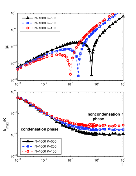
Figure 1: Simulation results of the network under Boltzmann limit for distribution $g(\epsilon)=C\epsilon^{\theta}$ with $\theta=0$. The upper panel is the plot of absolute value of chemical potential $\mu$ with temperature $T$ on a logarithmic scale, the lower panel is the fraction of total links occupied by the most connected nodes. The curves are plotted for the same number of nodes $N=1000$, but different number of total links: $K=500$ (open triangle with solid line), $K=200$ (open square with dashed line), and $K=100$ (open circle with dotted line), respectively. The numerical simulations are averaged over 50 runs.

The simulation results of our model in the classical limit are shown in Figs. 1 – 5. In Fig. 1, we show the relationship of absolute value of chemical potential $|\mu|$ with temperature parameter $T=1/\beta$, in upper panel. The curves represent networks with $N=1000$ and $K=500$, $200$, $100$, respectively. It can be seen clearly that there exist transitions in $|\mu|$, which means the chemical potential $\mu$ changes its sign, i.e., $\mu$ is positive in $T<T_{c}$ regime and negative in $T>T_{c}$ regime. The negativeness of $\mu$ in $T>T_{c}$ regime only has a formal similarity to that of the ideal Boltzmann gases, since, after all, the classical limit condition is not satisfied in the low temperature regime and hence no such condensation behavior in Boltzmann statistics.

The (non)condensation behavior is shown in the lower panel in Fig. 1. We can see that the fraction increases to unity gradually, as temperature decreases. Also, the critical temperature $T_{c}$ shifts towards to higher temperature when the ratio $K/N$ increases. In low temperature limit, the connectivity probability of non-growing network is primarily dominated by factor $e^{-\beta\epsilon_{i}}$ rather than $k_{i}$, which is similar to a network under the classical limit. As we already mentioned earlier, it should be noted that the non-condensation phase of classical limit network is different from the so called “FGR” phase of the fitness model in growing network. In non-condensation phase the connectivity probability of each node is randomly distributed over all energy levels. However, in FGR phase, for the nodes with higher fitness the connectivity degree increase more quickly than those nodes with lower fitness.

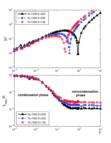
Figure 2: Similar to the Fig. 1, but for the distribution of energy level $g(\epsilon)=C\epsilon^{\theta}$ with $\theta=1$.

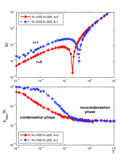
Figure 3: The comparisons of the absolute value of chemical potential, $|\mu|$ (upper panel), and $k_{max}/K$ (lower panel) with the same number of nodes ($N=1000$) and links ($K=200$), but with different energy level distributions $g(\epsilon)=C\epsilon^{\theta}$, $\theta=0$ (open diamond with solid lines), and $\theta=1$ (star with dashed lines).

Different distributions of energy level, $g(\epsilon)$, also influence the (non)condensation phase behavior under the classical limit. In our model, we employ the following form,

$$g(\epsilon)=C\epsilon^{\theta},$$ (13)

where $\theta$ is a parameter and $C$ is normalization factor. The simulations shown in Fig. 1 correspond to $\theta=0$, $C=1$, i.e., a uniform distribution. In Fig. 2, we show the simulation results of $|\mu|$ and $k_{max}/K$ for $\theta=1$, $C=2$. To illustrate clearly the effects of $g(\epsilon)$, in Fig. 3 we show the comparisions of the simulations with $\theta=0$ and $\theta=1$ for the same number of nodes and links ($N=1000$, $K=200$). The enhancement of critical transition temperature $T_{c}$ for distribution with $\theta=1$ is obvious.

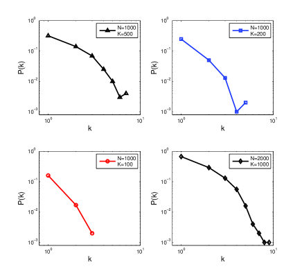
Figure 4: The connectivity degree distribution $P(k)$ vs. degree $k$ for $N=1000$, $K=500$ (open triangles), $200$ (open squares), $100$ (open circles) and $N=2000$, $K=1000$ (open diamonds) with distribution $g(\epsilon)=C\epsilon^{\theta}$, $\theta=0$ at temperature $T=0.2$.

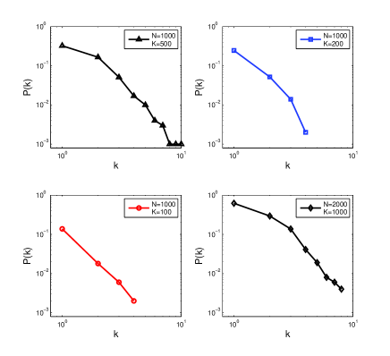
Figure 5: Similar to the Fig. 4 but for the distribution of energy levels $g(\epsilon)=C\epsilon^{\theta}$ with $\theta=1$.

We also plot the probability distribution of connectivity degree $P(k)$ at temperature $T=0.2$ for distributions with $\theta=0$ (Fig. 4) and $\theta=1$ (Fig. 5), respectively. The up left, up right and lower left panels in Fig. 4 and Fig. 5 correspond to the following number of nodes and links: $N=1000$ and $K=500$, $200$, $100$. With different number of nodes $N$ and links $K$ but the same ratios of $K/N$ as shown in the up left and lower right panels in Fig. 4 and Fig. 5, respectively, the distributions $P(k)$ (vs. $k$) are quite similar except for the fluctuation in tails. A particularly interesting observation is, at given temperature, it seems like the probability distributions of $k_{i}$ deviate from power-law distribution, as with the increase of the ratios $K/N$, which is clearly demonstrated in both figures. This significant difference from scale free network show some hints on the possible connection with recent observations: some real-world complex networks display a Weibull- or mixed-Weibull-power-law distribution Xu ; He07 ; Chen ; Chang ; Leskovec ; Seshadri . Although some models are proposed to explain (see, e.g., Ref. He07 ), the underlying mechanism for such distribution is worthy of further studying.

In conclusion, in present paper, we extend Bianconi-Barabási fitness model from growing complex networks to non-growing networks with fixed number of nodes and links. We fulfill numerical simulations and identify the corresponding “critical temperature” $T_{c}$. We also find that the “non-condensation phase” of our extension differs from FGR phase in B-B model, and the degree distribution $P(k)$ deviates from the power-law distribution at some temperatures.

Acknowledgements. The authors thank Prof. Albert-L. Barabási for discussions and acknowledge to National Natural Science Foundation of China (NSFC) for their support, under Contract No. 10875058.

References

- (1) D. J. Watts and S. H. Strogatz, Nature (London) 393, 440 (1998).
- (2) R. Albert and A.-L. Barabási, Rev. Mod. Phys. 74, 47 (2002).
- (3) D. J. Watts, Small Worlds: The Dynamics of Networks between Order and Randomness, Princeton University Press, Princeton, NJ, 1999.
- (4) S. N. Dorogovtsev and J. F. F. Mendes, Evolution of Networks, Oxford University Press, Oxford, 2003.
- (5) R. Pastor-Satorras, A. Vespignani, Evolution and Structure of the Internet: A Statistical Physics Approach, Cambridge University Press, Cambridge, 2004.
- (6) R. Albert and A.-L. Barabási, Phys. Rev. Lett. 85, 5234 (2000).
- (7) R. Guimerá, A. Díaz-Guilera, F. Vega-Redondo, A. Cabrales and A. Arenas, Phys. Rev. Lett. 89, 248701 (2002).
- (8) L. Donetti, P. I. Hurtado and M. A. Muñoz, Phys. Rev. Lett. 95, 188701 (2005).
- (9) A.-L. Barabási and R. Albert, Science 286, 509 (1999).
- (10) M. E. J. Newman, Phys. Rev. E 64, 025102 (2001).
- (11) H. Jeong, Z. Neda, A.-L. Barabási, Europhys. Lett. 61, 567 (2003).
- (12) S. N. Dorogovtsev, J. F. F. Mendes and J. G. Oliveira, Phys. Rev. E 73, 056122 (2006).
- (13) G. Bianconi and A.-L. Barabási, Europhys. Lett. 54, 436-442 (2001).
- (14) G. Bianconi and A.-L. Barabási, Phys. Rev. Lett. 86, 5632 (2001).
- (15) At least for the lowest energy level, there exists the possibility of a BEC phase transition. However, whether or not BE statistics holds for all energy levels, is still under investigations SZZ10 .
- (16) K. Huang, Statistical Mechanics, Wiley, Singapore, 1987.
- (17) K. Xu, L. Liu and X. Liang, arXiv:0908.0588 [cond-mat].
- (18) Y. He, G. Siganos, M. Faloutsos, S. V. Krishnamurthy, Proc. USENIX/SIGCOMM NSDI (2007).
- (19) Q. Chen, H. Chang, R. Govindan, S. Jamin, S. Shenker and W. Willinger, Proc. INFOCOM (2002).
- (20) H. Chang, S. Jamin and W. Willinger, Proc. INFOCOM (2006).
- (21) J. Leskovec and E. Horvitz, Proc. WWW (2008).
- (22) M. Seshadri, S. Machiraju, A. Sridharan, J. Bolot, C. Faloutsos and J. Leskove, Proc. SIGKDD (2008).
- (23) G. Su, Y. Zhang and X. Zhang, In preparation.