Inequities in the Shanks–Rényi Prime Number Race: An asymptotic formula for the densities

Abstract.

Chebyshev was the first to observe a bias in the distribution of primes in residue classes. The general phenomenon is that if $a$ is a nonsquare (mod $q$) and $b$ is a square (mod $q$), then there tend to be more primes congruent to $a{\text{\rm\ (mod~{}$q$)}}$ than $b{\text{\rm\ (mod~{}$q$)}}$ in initial intervals of the positive integers; more succinctly, there is a tendency for $\pi(x;q,a)$ to exceed $\pi(x;q,b)$. Rubinstein and Sarnak defined $\delta(q;a,b)$ to be the logarithmic density of the set of positive real numbers $x$ for which this inequality holds; intuitively, $\delta(q;a,b)$ is the “probability” that $\pi(x;q,a)>\pi(x;q,b)$ when $x$ is “chosen randomly”. In this paper, we establish an asymptotic series for $\delta(q;a,b)$ that can be instantiated with an error term smaller than any negative power of $q$. This asymptotic formula is written in terms of a variance $V(q;a,b)$ that is originally defined as an infinite sum over all nontrivial zeros of Dirichlet $L$-functions corresponding to characters (mod $q$); we show how $V(q;a,b)$ can be evaluated exactly as a finite expression. In addition to providing the exact rate at which $\delta(q;a,b)$ converges to $\frac{1}{2}$ as $q$ grows, these evaluations allow us to compare the various density values $\delta(q;a,b)$ as $a$ and $b$ vary modulo $q$; by analyzing the resulting formulas, we can explain and predict which of these densities will be larger or smaller, based on arithmetic properties of the residue classes $a$ and $b{\text{\rm\ (mod~{}$q$)}}$. For example, we show that if $a$ is a prime power and $a^{\prime}$ is not, then $\delta(q;a,1)<\delta(q;a^{\prime},1)$ for all but finitely many moduli $q$ for which both $a$ and $a^{\prime}$ are nonsquares. Finally, we establish rigorous numerical bounds for these densities $\delta(q;a,b)$ and report on extensive calculations of them, including for example the determination of all 117 density values that exceed $\frac{9}{10}$.

1. Introduction

We have known for over a century now that the prime numbers are asymptotically evenly distributed among the reduced residue classes modulo any fixed positive integer $q$. In other words, if $\pi(x;q,a)$ denotes the number of primes not exceeding $x$ that are congruent to $a{\text{\rm\ (mod~{}$q$)}}$, then $\lim_{x\to\infty}\pi(x;q,a)/\pi(x;q,b)=1$ for any integers $a$ and $b$ that are relatively prime to $q$. However, this information by itself is not enough to tell us about the distribution of values of the difference $\pi(x;q,a)-\pi(x;q,b)$, in particular whether this difference must necessarily take both positive and negative values. Several authors—notably Chebyshev in 1853 and Shanks [15] in 1959—observed that $\pi(x;4,3)$ has an extremely strong tendency to be greater than $\pi(x;4,1)$, and similar biases exist for other moduli as well. The general phenomenon is that $\pi(x;q,a)$ tends to exceed $\pi(x;q,b)$ when $a$ is a nonsquare modulo $q$ and $b$ is a square modulo $q$.

In 1994, Rubinstein and Sarnak [14] developed a framework for studying these questions that has proven to be quite fruitful. Define $\delta(q;a,b)$ to be the logarithmic density of the set of real numbers $x\geq 1$ satisfying $\pi(x;q,a)>\pi(x;q,b)$. (Recall that the logarithmic density of a set $S$ of positive real numbers is

$$\lim_{X\to\infty}\bigg{(}\frac{1}{\log X}\int\limits_{\begin{subarray}{c}1\leq x\leq X\\ x\in S\end{subarray}}\frac{dx}{x}\bigg{)},$$

or equivalently the natural density of the set $\{\log x\colon x\in S\}$.) Rubinstein and Sarnak investigated these densities under the following two hypotheses:

• The Generalized Riemann Hypothesis (GRH): all nontrivial zeros of Dirichlet $L$-functions have real part equal to $\frac{1}{2}$

• A linear independence hypothesis (LI): the nonnegative imaginary parts of these nontrivial zeros are linearly independent over the rationals

Under these hypotheses, they proved that the limit defining $\delta(q;a,b)$ always exists and is strictly between 0 and 1. Among other things, they also proved that $\delta(q;a,b)$ tends to $\frac{1}{2}$ as $q$ tends to infinity, uniformly for all pairs $a,b$ of distinct reduced residues (mod $q$).

In the present paper, we examine these densities $\delta(q;a,b)$ more closely. We are particularly interested in a quantitative statement of the rate at which $\delta(q;a,b)$ approaches $\frac{1}{2}$. In addition, computations show that for a fixed modulus $q$, the densities $\delta(q;a,b)$ vary as $a$ and $b$ range over nonsquares and squares modulo $q$, respectively. We are also interested in determining which pairs $a,b{\text{\rm\ (mod~{}$q$)}}$ give rise to larger or smaller values of $\delta(q;a,b)$, and especially in giving criteria that depend as directly as possible on $a$ and $b$ rather than on analytic data such as the zeros of Dirichlet $L$-functions.

Our first theorem, which is proved in Section 2.4, exhibits an asymptotic series for $\delta(q;a,b)$:

Theorem 1.1.

Assume GRH and LI. Let $q$ be a positive integer, and let $\rho(q)$ be the function defined in Definition 1.2. Let $a$ and $b$ be reduced residues (mod $q$) such that $a$ is a nonsquare (mod $q$) and $b$ is a square (mod $q$), and let $V(q;a,b)$ be the variance defined in Definition 1.3. Then for any nonnegative integer $K$,

$$\delta(q;a,b)=\frac{1}{2}+\frac{\rho(q)}{\sqrt{2\pi V(q;a,b)}}\sum_{\ell=0}^{K}\frac{1}{V(q;a,b)^{\ell}}\sum_{j=0}^{\ell}\rho(q)^{2j}s_{q;a,b}(\ell,j)+O_{K}\bigg{(}\frac{\rho(q)^{2K+3}}{V(q;a,b)^{K+3/2}}\bigg{)},$$ (1.1)

where the real numbers $s_{q;a,b}(\ell,j)$, which are bounded in absolute value by a function of $\ell$ uniformly in $q$, $a$, $b$, and $j$, are defined in Definition 2.23. In particular, $s_{q;a,b}(0,0)=1$, so that

$$\delta(q;a,b)=\frac{1}{2}+\frac{\rho(q)}{\sqrt{2\pi V(q;a,b)}}+O\bigg{(}\frac{\rho(q)^{3}}{V(q;a,b)^{3/2}}\bigg{)}.$$ (1.2)

We will see in Proposition 3.6 that $V(q;a,b)\sim 2\phi(q)\log q$, and so the error term in equation (1.1) is $\ll_{K,\varepsilon}1/q^{K+3/2-\varepsilon}$.

The assumption that $a$ is a nonsquare (mod $q$) and $b$ is a square (mod $q$) is natural in this context, reflecting the bias observed by Chebyshev. Rubinstein and Sarnak showed (assuming GRH and LI) that $\delta(q;b,a)+\delta(q;a,b)=1$; therefore if $a$ is a square (mod $q$) and $b$ is a nonsquare (mod $q$), the right-hand sides of the asymptotic formulas (1.1) and (1.2) become $\frac{1}{2}-\cdots$ instead of $\frac{1}{2}+\cdots$. Rubinstein and Sarnak also showed that $\delta(q;b,a)=\delta(q;a,b)=\frac{1}{2}$ if $a$ and $b$ are both squares or both nonsquares (mod $q$).

The definitions of $\rho(q)$ and of $V(q;a,b)$ are as follows:

Definition 1.2.

As usual, $\omega(q)$ denotes the number of distinct prime factors of $q$. Define $\rho(q)$ to be the number of real characters (mod $q$), or equivalently the index of the subgroup of squares in the full multiplicative group (mod $q$), or equivalently still the number of solutions of $x^{2}\equiv 1{\text{\rm\ (mod~{}$q$)}}$. An exercise in elementary number theory shows that

$$\rho(q)=\begin{cases}2^{\omega(q)},&\text{if }2\nmid q,\\ 2^{\omega(q)-1},&\text{if }2\mid q\text{ but }4\nmid q,\\ 2^{\omega(q)},&\text{if }4\mid q\text{ but }8\nmid q,\\ 2^{\omega(q)+1},&\text{if }8\mid q,\\ \end{cases}$$

which implies that $\rho(q)\ll_{\varepsilon}q^{\varepsilon}$ for every $\varepsilon>0$. $\diamondsuit$

Definition 1.3.

For any Dirichlet character $\chi{\text{\rm\ (mod~{}$q$)}}$, define

$$b(\chi)=\sum_{\begin{subarray}{c}\gamma\in{\mathbb{R}}\\ L(1/2+i\gamma,\chi)=0\end{subarray}}\frac{1}{\frac{1}{4}+\gamma^{2}}.$$

We adopt the convention throughout this paper that the zeros are listed with multiplicity in all such sums (though note that the hypothesis LI, when in force, implies that all such zeros are simple). For any reduced residues $a$ and $b{\text{\rm\ (mod~{}$q$)}}$, define

$$V(q;a,b)=\sum_{\chi{\text{\rm\ (mod~{}$q$)}}}|\chi(b)-\chi(a)|^{2}b(\chi).$$

We will see in Proposition 2.7 that $V(q;a,b)$ is the variance of a particular distribution associated with the difference $\pi(x;q,a)-\pi(x;q,b)$. $\diamondsuit$

As the asymptotic series in Theorem 1.1 depends crucially on the variance $V(q;a,b)$, we next give a formula for it (established in Section 3.2) that involves only a finite number of easily computed quantities:

Theorem 1.4.

Assume GRH. For any pair $a,b$ of distinct reduced residues modulo $q$,

$$V(q;a,b)=2\phi(q)\big{(}{\mathcal{L}}(q)+K_{q}(a-b)+\iota_{q}(-ab^{-1})\log 2\big{)}+2M^{*}(q;a,b),$$

where the functions ${\mathcal{L}}$, $K_{q}$, and $\iota_{q}$ are defined in Definition 1.5 and the quantity $M^{*}(q;a,b)$ is defined in Definition 1.6.

The definitions of these three arithmetic functions and of the analytic quantity $M^{*}$ are as follows:

Definition 1.5.

As usual, $\phi(q)$ denotes Euler’s totient function, and $\Lambda(q)$ denotes the von Mangoldt function, which takes the value $\log p$ if $q$ is a power of the prime $p$ and 0 otherwise. For any positive integer $q$, define

$${\mathcal{L}}(q)=\log q-\sum_{p\mid q}\frac{\log p}{p-1}+\frac{\Lambda(q)}{\phi(q)}-(\gamma_{0}+\log 2\pi),$$

where $\gamma_{0}=\lim_{x\to\infty}\big{(}\sum_{n\leq x}\frac{1}{n}-\log x\big{)}$ is Euler’s constant; it can be easily shown that ${\mathcal{L}}(q)$ is positive when $q\geq 43$. Note that ${\mathcal{L}}(q)=\log(q/2\pi e^{\gamma_{0}})$ when $q$ is prime and that ${\mathcal{L}}(q)=\log q+O(\log\log q)$ for any integer $q\geq 3$. Also let

$$\iota_{q}(n)=\begin{cases}1,&\text{if }n\equiv 1{\text{\rm\ (mod~{}$q$)}},\\ 0,&\text{if }n\not\equiv 1{\text{\rm\ (mod~{}$q$)}}\end{cases}$$

denote the characteristic function of the integers that are congruent to 1 (mod $q$). Finally, define

$$K_{q}(n)=\frac{\Lambda(q/(q,n))}{\phi(q/(q,n))}-\frac{\Lambda(q)}{\phi(q)}.$$

Note that these last two functions depend only on the residue class of $n$ modulo $q$. For this reason, in expressions such as $\iota_{q}(n^{-1})$ or $K_{q}(n^{-1})$, the argument $n^{-1}$ is to be interpreted as an integer that is the multiplicative inverse of $n{\text{\rm\ (mod~{}$q$)}}$. In addition, note that $K_{q}(n)\geq 0$, since the only way that the second term can contribute is if $q$ is a prime power, in which case the first term contributes at least as much. On the other hand $K_{q}$ is bounded above, since if $q/(q,n)$ is a power of the prime $p$ then $K_{q}(n)\leq(\log p)/(p-1)\leq\log 2$. Note also that $K_{q}(n)=0$ when $(n,q)=1$. $\diamondsuit$

Definition 1.6.

As usual, $L(s,\chi)=\sum_{n=1}^{\infty}\chi(n)n^{-s}$ denotes the $L$-function associated to the Dirichlet character $\chi$. Given such a character $\chi{\text{\rm\ (mod~{}$q$)}}$, let $q^{*}$ denote its conductor (that is, the smallest integer $d$ such that $\chi$ is induced by a character modulo $d$), and let $\chi^{*}$ be the unique character modulo $q^{*}$ that induces $\chi$. Now define

$$M^{*}(q;a,b)=\sum_{\begin{subarray}{c}\chi{\text{\rm\ (mod~{}$q$)}}\\ \chi\neq\chi_{0}\end{subarray}}|\chi(a)-\chi(b)|^{2}\frac{L^{\prime}(1,\chi^{*})}{L(1,\chi^{*})}$$

and

$$M(q;a,b)=\sum_{\begin{subarray}{c}\chi{\text{\rm\ (mod~{}$q$)}}\\ \chi\neq\chi_{0}\end{subarray}}|\chi(a)-\chi(b)|^{2}\frac{L^{\prime}(1,\chi)}{L(1,\chi)}.$$

$\diamondsuit$

The formula for $V(q;a,b)$ in Theorem 1.4 is exact and hence well suited for computations. For theoretical purposes, however, we need a better understanding of $M^{*}(q;a,b)$, which our next theorem (proved in Section 3.3) provides:

Theorem 1.7.

Assume GRH. For any pair $a,b$ of distinct reduced residues modulo $q$, let $r_{1}$ and $r_{2}$ denote the least positive residues of $ab^{-1}$ and $ba^{-1}{\text{\rm\ (mod~{}$q$)}}$, and let the quantity $H(q;a,b)$ be defined in Definition 1.8. Then

$$M^{*}(q;a,b)=\phi(q)\bigg{(}\frac{\Lambda(r_{1})}{r_{1}}+\frac{\Lambda(r_{2})}{r_{2}}+H(q;a,b)+O\bigg{(}\frac{\log^{2}q}{q}\bigg{)}\bigg{)},$$

where the implied constant is absolute.

(The unexpected appearance of the specific integers $r_{1}$ and $r_{2}$, in a formula for a quantity depending upon entire residue classes (mod $q$), is due to the approximation of infinite series by their first terms—see Proposition 3.12.) The quantity $H(q;a,b)$ is usually quite small, unless there is an extreme coincidence in the locations of $a$ and $b$ relative to the prime divisors of $q$, which would be reflected in a small value of the quantity $e(q;p,r)$ defined as follows:

Definition 1.8.

Given an integer $q$ and a prime $p$, let $\nu\geq 0$ be the integer such that $p^{\nu}\parallel q$ (that is, $p^{\nu}\mid q$ but $p^{\nu+1}\nmid q$). For any reduced residue $r{\text{\rm\ (mod~{}$q$)}}$, define $e(q;p,r)=\min\{e\geq 1\colon p^{e}\equiv r^{-1}{\text{\rm\ (mod~{}$q/p^{\nu}$)}}\},$ and define

$$h(q;p,r)=\frac{1}{\phi(p^{\nu})}\frac{\log p}{p^{e(q;p,r)}}.$$

When $r$ is not in the multiplicative subgroup generated by $p{\text{\rm\ (mod~{}$q/p^{\nu}$)}}$, we make the convention that $e(q;p,r)=\infty$ and $h(q;p,r)=0$. Finally, for any integers $a$ and $b$, define

$$H(q;a,b)=\sum_{p\mid q}\big{(}h(q;p,ab^{-1})+h(q;p,ba^{-1})\big{)}.$$

Note that if $q=p^{\nu}$ is a prime power, then $h(q;p,r)=(\log p)/p^{\nu}(p-1)$ is independent of $r$, which implies that $H(q;a,b)\ll(\log q)/q$ when $q$ is a prime power. $\diamondsuit$

The extremely small relative error in Theorem 1.1 implies that the formula given therein is useful even for moderate values of $q$. The following corollary of the above theorems, the proof of which is given in Section 4.1, is useful only for large $q$ due to a worse error term. It has the advantage, however, of isolating the fine-scale dependence of $\delta(q;a,b)$ on the residue classes $a$ and $b$ from its primary dependence on the modulus $q$:

Corollary 1.9.

Assume GRH and LI. Let $q\geq 43$ be an integer. Let $a$ and $b$ be reduced residues (mod $q$) such that $a$ is a nonsquare (mod $q$) and $b$ is a square (mod $q$), and let $r_{1}$ and $r_{2}$ denote the least positive residues of $ab^{-1}$ and $ba^{-1}{\text{\rm\ (mod~{}$q$)}}$. Then

$$\delta(q;a,b)=\frac{1}{2}+\frac{\rho(q)}{2\sqrt{\pi\phi(q){\mathcal{L}}(q)}}\bigg{(}1-\frac{\Delta(q;a,b)}{2{\mathcal{L}}(q)}+O\bigg{(}\frac{1}{\log^{2}q}\bigg{)}\bigg{)},$$ (1.3)

where

$$\Delta(q;a,b)=K_{q}(a-b)+\iota_{q}(-ab^{-1})\log 2+\frac{\Lambda(r_{1})}{r_{1}}+\frac{\Lambda(r_{2})}{r_{2}}+H(q;a,b)$$ (1.4)

(here, the functions ${\mathcal{L}}$, $K_{q}$, and $\iota_{q}$ are defined in Definition 1.5, and $H$ is defined in Definition 1.8). Moreover, $\Delta(q;a,b)$ is nonnegative and bounded above by an absolute constant.

Armed with this knowledge of the delicate dependence of $\delta(q;a,b)$ on the residue classes $a$ and $b$, we are actually able to “race races”, that is, investigate inequalities between various values of $\delta(q;a,b)$ as $q$ increases. We remark that Feuerverger and Martin [5, Theorem 2(b)] showed that $\delta(q;a,b)=\delta(q;ab^{-1},1)$ for any square $b{\text{\rm\ (mod~{}$q$)}}$, and so it often suffices to consider only the densities $\delta(q;a,1)$. Some surprising inequalities come to light when we fix the residue class $a$ and allow the modulus $q$ to vary (among moduli relatively prime to $a$ for which $a$ is a nonsquare). Our next theorem, which is a special case of Corollary 4.3 derived in Section 4.2, demonstrates some of these inequalities:

Theorem 1.10.

Assume GRH and LI.

• For any integer $a\neq-1$, we have $\delta(q;-1,1)<\delta(q;a,1)$ for all but finitely many integers $q$ with $(q,a)=1$ such that both $-1$ and $a$ are nonsquares (mod $q$).

• If $a$ is a prime power and $a^{\prime}\neq-1$ is an integer that is not a prime power, then $\delta(q;a,1)<\delta(q;a^{\prime},1)$ for all but finitely many integers $q$ with $(q,aa^{\prime})=1$ such that both $a$ and $a^{\prime}$ are nonsquares (mod $q$).

• If $a$ and $a^{\prime}$ are prime powers with $\Lambda(a)/a>\Lambda(a^{\prime})/a^{\prime}$, then $\delta(q;a,1)<\delta(q;a^{\prime},1)$ for all but finitely many integers $q$ with $(q,aa^{\prime})=1$ such that both $a$ and $a^{\prime}$ are nonsquares (mod $q$).

Finally, these results have computational utility as well. A formula [5, equation (2-57)] for calculating the value of $\delta(q;a,b)$ is known. However, this formula requires knowledge of a large number of zeros of all Dirichlet $L$-functions associated to characters (mod $q$) even to estimate via numerical integration; therefore it becomes unwieldy to use the formula when $q$ becomes large. On the other hand, the asymptotic series in Theorem 1.1 can be made completely effective, and the calculation of $V(q;a,b)$ is painless thanks to Theorem 1.4. Therefore the densities $\delta(q;a,b)$ can be individually calculated, and collectively bounded, for large $q$.

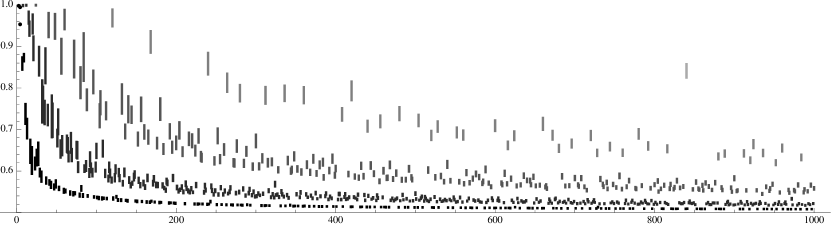
Figure 1. All densities $\delta(q;a,b)$ with $q\leq 1000$

For example, the values of $\delta(q;a,b)$ for all moduli up to $1000$ are plotted in Figure 1. The modulus $q$ is given on the horizontal axis; the vertical line segment plotted for each $q$ extends between the maximal and minimal values of $\delta(q;a,b)$, as $a$ runs over all nonsquares (mod $q$) and $b$ runs over all squares (mod $q$). (Of course both $a$ and $b$ should be relatively prime to $q$. We also omit moduli of the form $q\equiv 2{\text{\rm\ (mod~{}$4$)}}$, since the distribution of primes into residue classes modulo such $q$ is the same as their distribution into residue classes modulo $q/2$.)

The values shown in Figure 1 organize themselves into several bands; each band corresponds to a constant value of $\rho(q)$, the effect of which on the density $\delta(q;a,b)$ can be clearly seen in the second term on the right-hand side of equation (1.3). For example, the lowest (and darkest) band corresponds to moduli $q$ for which $\rho(q)=2$, meaning odd primes and their powers (as well as $q=4$); the second-lowest band corresponds to those moduli for which $\rho(q)=4$, consisting essentially of numbers with two distinct prime factors; and so on, with the first modulus $q=840$ for which $\rho(q)=32$ (the segment closest to the upper right-hand corner of the graph) hinting at the beginning of a fifth such band. Each band decays roughly at a rate of $1/\sqrt{q\log q}$, as is also evident from the aforementioned term of equation (1.3).

To give one further example of these computations, which we describe in Section 5.4, we are able to find the largest values of $\delta(q;a,b)$ that ever occur. (All decimals listed in this paper are rounded off in the last decimal place.)

Theorem 1.11.

Assume GRH and LI. The ten largest values of $\delta(q;a,b)$ are given in Table 1.

Table 1. The top 10 most unfair prime number races

$q$	$a$	$b$	$\delta(q;a,b)$
24	5	1	0.999988
24	11	1	0.999983
12	11	1	0.999977
24	23	1	0.999889
24	7	1	0.999834
24	19	1	0.999719
8	3	1	0.999569
12	5	1	0.999206
24	17	1	0.999125
3	2	1	0.999063

Our approach expands upon the seminal work of Rubinstein and Sarnak [14], who introduced a random variable whose distribution encapsulates the information needed to understand $\pi(x;q,a)-\pi(x;q,b)$. We discuss these random variables, formulas and estimates for their characteristic functions (that is, Fourier transforms), and the subsequent derivation of the asymptotic series from Theorem 1.1 in Section 2. In Section 3 we demonstrate how to transform the variance $V(q;a,b)$ from an infinite sum into a finite expression; we can even calculate it extremely precisely using only arithmetic (rather than analytic) information. We also show how the same techniques can be used to establish a central limit theorem for the aforementioned distributions, and we outline how modifications of our arguments can address the two-way race between all nonresidues and all residues (mod $q$). We investigate the fine-scale effect of the particular residue classes $a$ and $b$ upon the density $\delta(q;a,b)$ in Section 4; we also show how a similar analysis can explain a “mirror image” phenomenon noticed by Bays and Hudson [2]. Finally, Section 5 is devoted to explicit estimates and a description of our computations of the densities and the resulting conclusions, including Theorem 1.11.

Acknowledgments

The authors thank Brian Conrey and K. Soundararajan for suggesting proofs of Lemma 2.8(c) and Proposition 3.10, respectively, that were superior to our original proofs. We also thank Andrew Granville for indicating how to improve the error term in Proposition 3.11, as well as Colin Myerscough for correcting a numerical error in Proposition 2.14 that affected our computations in Sections 5.3–5.4. Robert Rumely and Michael Rubinstein provided lists of zeros of Dirichlet $L$-functions and the appropriate software to compute these zeros, which are needed for the calculations of the densities in Section 5, and we thank them as well. Finally, we express our gratitude to our advisors past and present, Andrew Granville, Hugh Montgomery, and Trevor Wooley, both for their advice about this paper and for their guidance in general. Le premier auteur est titulaire d’une bourse doctorale du Conseil de recherches en sciences naturelles et en génie du Canada. The second author was supported in part by grants from the Natural Sciences and Engineering Research Council of Canada.

2. The asymptotic series for the density $\delta(q;a,b)$

The ultimate goal of this section is to prove Theorem 1.1. We begin in Section 2.1 by describing a random variable whose distribution is the same as the limiting logarithmic distribution of a suitably normalized version of $\pi(x;q,a)-\pi(x;q,b)$, as well as calculating its variance. This approach is the direct descendant of that of Rubinstein and Sarnak [14]; one of our main innovations is the exact evaluation of the variance $V(q;a,b)$ in a form that does not involve the zeros of Dirichlet $L$-functions. In Section 2.2 we derive the formula for the characteristic function (Fourier transform) of that random variable; this formula is already known, but our derivation is slightly different and allows us to write the characteristic function in a convenient form (see Proposition 2.12). We then use our knowledge of the characteristic function to write the density $\delta(q;a,b)$ as the truncation of an infinite integral in Section 2.3, where the error terms are explicitly bounded using knowledge of the counting function $N(T,\chi)$ of zeros of Dirichlet $L$-functions. Finally, we derive the asymptotic series from Theorem 1.1 from this truncated integral formula in Section 2.4.

2.1. Distributions and random variables

We begin by describing random variables related to the counting functions of primes in arithmetic progressions. As is typical when considering primes in arithmetic progressions, we first consider expressions built out of Dirichlet characters.

Definition 2.1.

For any Dirichlet character $\chi$ such that GRH holds for $L(s,\chi)$, define

$$E(x,\chi)=\sum_{\begin{subarray}{c}\gamma\in{\mathbb{R}}\\ L(1/2+i\gamma,\chi)=0\end{subarray}}\frac{x^{i\gamma}}{\frac{1}{2}+i\gamma}.$$

This sum does not converge absolutely, but (thanks to GRH and the functional equation for Dirichlet $L$-functions) it does converge conditionally when interpreted as the limit of $\sum_{|\gamma|<T}$ as $T$ tends to infinity. All untruncated sums over zeros of Dirichlet $L$-functions in this paper should be similarly interpreted. $\diamondsuit$

Definition 2.2.

For any real number $\gamma$, let $Z_{\gamma}$ denote a random variable that is uniformly distributed on the unit circle, and let $X_{\gamma}$ denote the random variable that is the real part of $Z_{\gamma}$. We stipulate that the collection $\{Z_{\gamma}\}_{\gamma\geq 0}$ is independent and that $Z_{-\gamma}=\overline{Z_{\gamma}}$; this implies that the collection $\{X_{\gamma}\}_{\gamma\geq 0}$ is also independent and that $X_{-\gamma}=X_{\gamma}$. $\diamondsuit$

By the limiting logarithmic distribution of a real-valued function $f(t)$, we mean the measure $d\nu$ having the property that the limiting logarithmic density of the set of positive real numbers such that $f(t)$ lies between $\alpha$ and $\beta$ is $\int_{\alpha}^{\beta}d\nu$ for any interval $(\alpha,\beta)$.

Proposition 2.3.

Assume LI. Let $\{c_{\chi}\colon\chi{\text{\rm\ (mod~{}$q$)}}\}$ be a collection of complex numbers, indexed by the Dirichlet characters (mod $q$), satisfying $c_{\bar{\chi}}=\overline{c_{\chi}}$. The limiting logarithmic distribution of the function

$$\sum_{\chi{\text{\rm\ (mod~{}$q$)}}}c_{\chi}E(x,\chi)$$

is the same as the distribution of the random variable

$$2\sum_{\chi{\text{\rm\ (mod~{}$q$)}}}|c_{\chi}|\sum_{\begin{subarray}{c}\gamma>0\\ L(1/2+i\gamma,\chi)=0\end{subarray}}\frac{X_{\gamma}}{\sqrt{\frac{1}{4}+\gamma^{2}}}.$$

Proof.

We have

$$\sum_{\chi{\text{\rm\ (mod~{}$q$)}}}c_{\chi}E(x,\chi) =\lim_{T\to\infty}\sum_{\chi{\text{\rm\ (mod~{}$q$)}}}c_{\chi}\sum_{\begin{subarray}{c}|\gamma|<T\\ L(1/2+i\gamma,\chi)=0\end{subarray}}\frac{x^{i\gamma}}{\frac{1}{2}+i\gamma}$$

$$=\lim_{T\to\infty}\sum_{\chi{\text{\rm\ (mod~{}$q$)}}}c_{\chi}\bigg{(}\sum_{\begin{subarray}{c}0<\gamma<T\\ L(1/2+i\gamma,\chi)=0\end{subarray}}\frac{x^{i\gamma}}{\frac{1}{2}+i\gamma}+\sum_{\begin{subarray}{c}-T<\gamma<0\\ L(1/2+i\gamma,\chi)=0\end{subarray}}\frac{x^{i\gamma}}{\frac{1}{2}+i\gamma}\bigg{)}.$$

(The assumption of LI precludes the possibility that $\gamma=0$.) By the functional equation, the zeros of $L(s,\chi)$ below the real axis correspond to those of $L(s,\bar{\chi})$ above the real axis. Therefore

$$\sum_{\chi{\text{\rm\ (mod~{}$q$)}}}c_{\chi}E(x,\chi) =\lim_{T\to\infty}\sum_{\chi{\text{\rm\ (mod~{}$q$)}}}c_{\chi}\bigg{(}\sum_{\begin{subarray}{c}0<\gamma<T\\ L(1/2+i\gamma,\chi)=0\end{subarray}}\frac{x^{i\gamma}}{\frac{1}{2}+i\gamma}+\sum_{\begin{subarray}{c}0<\gamma<T\\ L(1/2+i\gamma,\bar{\chi})=0\end{subarray}}\frac{x^{-i\gamma}}{\frac{1}{2}-i\gamma}\bigg{)}$$ (2.1)

$$=\lim_{T\to\infty}\bigg{(}\sum_{\chi{\text{\rm\ (mod~{}$q$)}}}c_{\chi}\sum_{\begin{subarray}{c}0<\gamma<T\\ L(1/2+i\gamma,\chi)=0\end{subarray}}\frac{x^{i\gamma}}{\frac{1}{2}+i\gamma}+\sum_{\chi{\text{\rm\ (mod~{}$q$)}}}\overline{c_{\bar{\chi}}\sum_{\begin{subarray}{c}0<\gamma<T\\ L(1/2+i\gamma,\bar{\chi})=0\end{subarray}}\frac{x^{i\gamma}}{\frac{1}{2}+i\gamma}}\bigg{)}.$$

Reindexing this last sum by replacing $\bar{\chi}$ by $\chi$, we obtain

$$\sum_{\chi{\text{\rm\ (mod~{}$q$)}}}c_{\chi}E(x,\chi) =\lim_{T\to\infty}\bigg{(}\sum_{\chi{\text{\rm\ (mod~{}$q$)}}}c_{\chi}\sum_{\begin{subarray}{c}0<\gamma<T\\ L(1/2+i\gamma,\chi)=0\end{subarray}}\frac{x^{i\gamma}}{\frac{1}{2}+i\gamma}+\sum_{\chi{\text{\rm\ (mod~{}$q$)}}}\overline{c_{\chi}\sum_{\begin{subarray}{c}0<\gamma<T\\ L(1/2+i\gamma,\chi)=0\end{subarray}}\frac{x^{i\gamma}}{\frac{1}{2}+i\gamma}}\bigg{)}$$

$$=\lim_{T\to\infty}2\mathop{\rm Re}\bigg{(}\sum_{\chi{\text{\rm\ (mod~{}$q$)}}}c_{\chi}\sum_{\begin{subarray}{c}0<\gamma<T\\ L(1/2+i\gamma,\chi)=0\end{subarray}}\frac{x^{i\gamma}}{\frac{1}{2}+i\gamma}\bigg{)}$$ (2.2)

$$=2\lim_{T\to\infty}\sum_{\chi{\text{\rm\ (mod~{}$q$)}}}|c_{\chi}|\mathop{\rm Re}\bigg{(}\sum_{\begin{subarray}{c}0<\gamma<T\\ L(1/2+i\gamma,\chi)=0\end{subarray}}\frac{e^{i\gamma\log x}\theta_{\chi,\gamma}}{\sqrt{\frac{1}{4}+\gamma^{2}}}\bigg{)},$$

where $\theta_{\chi,\gamma}=c_{\chi}|\frac{1}{2}+i\gamma|/|c_{\chi}|(\frac{1}{2}+i\gamma)$ is a complex number of modulus 1. The quantity $e^{i\gamma\log x}\theta_{\chi,\gamma}$ is uniformly distributed (as a function of $\log x$) on the unit circle as $x$ tends to infinity, and hence its limiting logarithmic distribution is the same as the distribution of $Z_{\gamma}$. Since the various $\gamma$ in each inner sum are linearly independent over the rationals by LI, the tuple $(e^{i\gamma\log x}\theta_{\chi,\gamma})_{0<\gamma<T}$ is uniformly distributed in the $N(T,\chi)$-dimensional torus by Kronecker’s theorem. Therefore the limiting logarithmic distribution of the sum

$$\sum_{\begin{subarray}{c}0<\gamma<T\\ L(1/2+i\gamma,\chi)=0\end{subarray}}\frac{e^{i\gamma\log x}\theta_{\chi,\gamma}}{\sqrt{\frac{1}{4}+\gamma^{2}}}$$

is the same as the distribution of the random variable

$$\sum_{\begin{subarray}{c}0<\gamma<T\\ L(1/2+i\gamma,\chi)=0\end{subarray}}\frac{Z_{\gamma}}{\sqrt{\frac{1}{4}+\gamma^{2}}}.$$

Finally, the work of Rubinstein and Sarnak [14, Section 3.1] shows that the limiting logarithmic distribution of

$$\sum_{\chi{\text{\rm\ (mod~{}$q$)}}}c_{\chi}E(x,\chi)=2\lim_{T\to\infty}\sum_{\chi{\text{\rm\ (mod~{}$q$)}}}|c_{\chi}|\mathop{\rm Re}\bigg{(}\sum_{\begin{subarray}{c}0<\gamma<T\\ L(1/2+i\gamma,\chi)=0\end{subarray}}\frac{e^{i\gamma\log x}\theta_{\chi,\gamma}}{\sqrt{\frac{1}{4}+\gamma^{2}}}\bigg{)}$$

is the same as the distribution of the random variable

$$\sum_{\chi{\text{\rm\ (mod~{}$q$)}}}c_{\chi}E(x,\chi) =2\lim_{T\to\infty}\sum_{\chi{\text{\rm\ (mod~{}$q$)}}}|c_{\chi}|\sum_{\begin{subarray}{c}0<\gamma<T\\ L(1/2+i\gamma,\chi)=0\end{subarray}}\frac{X_{\gamma}}{\sqrt{\frac{1}{4}+\gamma^{2}}}$$

$$=2\sum_{\chi{\text{\rm\ (mod~{}$q$)}}}|c_{\chi}|\sum_{\begin{subarray}{c}\gamma>0\\ L(1/2+i\gamma,\chi)=0\end{subarray}}\frac{X_{\gamma}}{\sqrt{\frac{1}{4}+\gamma^{2}}},$$

the convergence of this last limit being ensured by the fact that the $X_{\gamma}$ are bounded and that each of the sums

$$\sum_{\begin{subarray}{c}\gamma>0\\ L(1/2+i\gamma,\chi)=0\end{subarray}}\bigg{(}\frac{1}{\sqrt{\frac{1}{4}+\gamma^{2}}}\bigg{)}^{2}\leq b(\chi)$$

is finite. This establishes the lemma. ∎

We shall have further occasion to change the indexing of sums, between over all $\gamma$ and over only positive $\gamma$, in the same manner as in equations (2.1) and (2.2); henceforth we shall justify such changes “by the functional equation for Dirichlet $L$-functions” and omit the intermediate steps.

Definition 2.4.

For any relative prime integers $q$ and $a$, define

$$c(q;a)=-1+\#\{x{\text{\rm\ (mod~{}$q$)}}\colon x^{2}\equiv a{\text{\rm\ (mod~{}$q$)}}\}.$$

Note that $c(q;a)$ takes only the values $-1$ and $\rho(q)-1$. Now, with $X_{\gamma}$ as defined in Definition 2.2, define the random variable

$$X_{q;a,b}=c(q,b)-c(q,a)+2\sum_{\chi{\text{\rm\ (mod~{}$q$)}}}|\chi(b)-\chi(a)|\sum_{\begin{subarray}{c}\gamma>0\\ L(1/2+i\gamma,\chi)=0\end{subarray}}\frac{X_{\gamma}}{\sqrt{\frac{1}{4}+\gamma^{2}}}.$$

Note that the expectation of the random variable $X_{q;a,b}$ is either $\pm\rho(q)$ or 0, depending on the values of $c(q,a)$ and $c(q,b)$. $\diamondsuit$

Definition 2.5.

With $\pi(x;q,a)=\#\{p\leq x\colon p\text{ prime, }p\equiv a{\text{\rm\ (mod~{}$q$)}}\}$ denoting the counting function of primes in the arithmetic progression $a{\text{\rm\ (mod~{}$q$)}}$, define the normalized error term

$$E(x;q,a)=\frac{\log x}{\sqrt{x}}\big{(}\phi(q)\pi(x;q,a)-\pi(x)\big{)}.$$

$\diamondsuit$

The next proposition characterizes the limiting logarithmic distribution of the difference of two of these normalized counting functions.

Proposition 2.6.

Assume GRH and LI. Let $a$ and $b$ be reduced residues modulo $q$. The limiting logarithmic distribution of $E(x;q,a)-E(x;q,b)$ is the same as the distribution of the random variable $X_{q;a,b}$ defined in Definition 2.4.

Remark.

Since $\delta(q;a,b)$ is defined to be the logarithmic density of those real numbers $x$ for which $\pi(x;q,a)>\pi(x;q,b)$, or equivalently for which $E(x;q,a)>E(x;q,b)$, we see that $\delta(q;a,b)$ equals the probability that $X_{q;a,b}$ is greater than 0. However, we never use this fact directly in the present paper, instead quoting from [5] a consequence of that fact in equation (2.10) below.

Proof.

As is customary, define

$$\psi(x,\chi)=\sum_{n\leq x}\chi(n)\Lambda(n)$$

A consequence of the explicit formula for $\psi(x,\chi)$ that arises from the analytic proof of the prime number theorem for arithmetic progressions ([11, Corollary 12.11] combined with [11, (12.12)]) is that for $\chi\neq\chi_{0}$,

$$\psi(x,\chi)=-\sum_{\begin{subarray}{c}\gamma\in{\mathbb{R}}\\ L(1/2+i\gamma,\chi)=0\end{subarray}}\frac{x^{1/2+i\gamma}}{\frac{1}{2}+i\gamma}+O(\log q\cdot\log x)$$

under the assumption of GRH. We also know [14, Lemma 2.1] that

$$E(x;q,a)=-c(q,a)+\sum_{\begin{subarray}{c}\chi{\text{\rm\ (mod~{}$q$)}}\\ \chi\neq\chi_{0}\end{subarray}}\bar{\chi}(a)\frac{\psi(x,\chi)}{\sqrt{x}}+O_{q}\bigg{(}\frac{1}{\log x}\bigg{)}.$$ (2.3)

Combining these last two equations with Definition 2.1 for $E(x,\chi)$, we obtain

$$E(x;q,a)=-c(q,a)-\sum_{\begin{subarray}{c}\chi{\text{\rm\ (mod~{}$q$)}}\\ \chi\neq\chi_{0}\end{subarray}}\bar{\chi}(a)E(x,\chi)+O_{q}\bigg{(}\frac{1}{\log x}\bigg{)}.$$

We therefore see that

$$E(x;q,a)-E(x;q,b)=c(q,b)-c(q,a)+\sum_{\chi{\text{\rm\ (mod~{}$q$)}}}(\bar{\chi}(b)-\bar{\chi}(a))E(x,\chi)+O_{q}\bigg{(}\frac{1}{\log x}\bigg{)}$$

(where we have added in the $\chi=\chi_{0}$ term for convenience). The error term tends to zero as $x$ grows and thus doesn’t affect the limiting distribution, and the constant $c(q,b)-c(q,a)$ is independent of $x$. Therefore, by Proposition 2.3, the limiting logarithmic distribution of $E(x;q,a)-E(x;q,b)$ is the same as the distribution of the random variable

$$c(q,b)-c(q,a)+2\sum_{\chi{\text{\rm\ (mod~{}$q$)}}}|\bar{\chi}(b)-\bar{\chi}(a)|\sum_{\begin{subarray}{c}\gamma>0\\ L(1/2+i\gamma,\chi)=0\end{subarray}}\frac{X_{\gamma}}{\sqrt{\frac{1}{4}+\gamma^{2}}}.$$

Since $|\bar{\chi}(b)-\bar{\chi}(a)|=|\chi(b)-\chi(a)|$, this last expression is exactly the random variable $X_{q;a,b}$ as claimed. ∎

To conclude this section, we calculate the variance of the random variable $X_{q;a,b}$.

Proposition 2.7.

Assume LI. Let $\{c_{\chi}\colon\chi{\text{\rm\ (mod~{}$q$)}}\}$ be a collection of complex numbers satisfying $c_{\bar{\chi}}=\overline{c_{\chi}}$. For any constant $\mu$, the variance of the random variable

$$\mu+2\sum_{\chi{\text{\rm\ (mod~{}$q$)}}}c_{\chi}\sum_{\begin{subarray}{c}\gamma>0\\ L(1/2+i\gamma,\chi)=0\end{subarray}}\frac{X_{\gamma}}{\sqrt{\frac{1}{4}+\gamma^{2}}}$$ (2.4)

equals $\sum_{\chi{\text{\rm\ (mod~{}$q$)}}}|c_{\chi}|^{2}b(\chi),$ where $b(\chi)$ was defined in Definition 1.3. In particular, the variance of the random variable $X_{q;a,b}$ defined in Definition 2.4 is equal to the quantity $V(q;a,b)$ defined in Definition 1.3.

Proof.

The random variables $\{X_{\gamma}\colon\gamma>0\}$ form an independent collection by definition; it is important to note that no single variable $X_{\gamma}$ can correspond to multiple characters $\chi$, due to the assumption of LI. The variance of the sum (2.4) is therefore simply the sum of the individual variances, that is,

$$\sigma^{2}\bigg{(}2\sum_{\chi{\text{\rm\ (mod~{}$q$)}}}|c_{\chi}|\sum_{\begin{subarray}{c}\gamma>0\\ L(1/2+i\gamma,\chi)=0\end{subarray}}\frac{X_{\gamma}}{\sqrt{\frac{1}{4}+\gamma^{2}}}\bigg{)}=4\sum_{\chi{\text{\rm\ (mod~{}$q$)}}}|c_{\chi}|^{2}\sum_{\begin{subarray}{c}\gamma>0\\ L(1/2+i\gamma,\chi)=0\end{subarray}}\frac{\sigma^{2}(X_{\gamma})}{\frac{1}{4}+\gamma^{2}}.$$

The variance of any $X_{\gamma}$ is $\frac{1}{2}$, and so this last expression equals

$$2\sum_{\chi{\text{\rm\ (mod~{}$q$)}}}|c_{\chi}|^{2}\sum_{\begin{subarray}{c}\gamma>0\\ L(1/2+i\gamma,\chi)=0\end{subarray}}\frac{1}{\frac{1}{4}+\gamma^{2}}$$

$$\qquad{}=\sum_{\chi{\text{\rm\ (mod~{}$q$)}}}|c_{\chi}|^{2}\sum_{\begin{subarray}{c}\gamma>0\\ L(1/2+i\gamma,\chi)=0\end{subarray}}\frac{1}{\frac{1}{4}+\gamma^{2}}+\sum_{\chi{\text{\rm\ (mod~{}$q$)}}}|c_{\chi}|^{2}\sum_{\begin{subarray}{c}\gamma<0\\ L(1/2+i\gamma,\bar{\chi})=0\end{subarray}}\frac{1}{\frac{1}{4}+\gamma^{2}}$$

$$\qquad{}=\sum_{\chi{\text{\rm\ (mod~{}$q$)}}}|c_{\chi}|^{2}\sum_{\begin{subarray}{c}\gamma\in{\mathbb{R}}\\ L(1/2+i\gamma,\chi)=0\end{subarray}}\frac{1}{\frac{1}{4}+\gamma^{2}}=\sum_{\chi{\text{\rm\ (mod~{}$q$)}}}|c_{\chi}|^{2}b(\chi)$$

by the functional equation for Dirichlet $L$-functions. The fact that $V(q;a,b)$ is the variance of $X_{q;a,b}$ now follows directly from their definitions. ∎

2.2. Calculating the characteristic function

The characteristic function $\hat{X}_{q;a,b}(z)$ of the random variable $X_{q;a,b}$ will be extremely important to our analysis of the density $\delta(q;a,b)$. To derive the formula for this characteristic function, we begin by setting down some relevant facts about the standard Bessel function $J_{0}$ of order zero. Specifically, we collect in the following lemma some useful information about the power series coefficients $\lambda_{n}$ for

$$\log J_{0}(z)=\sum_{n=0}^{\infty}\lambda_{n}z^{n},$$ (2.5)

which is valid for $|z|\leq\frac{12}{5}$ since $J_{0}$ has no zeros in a disk of radius slightly larger than $\frac{12}{5}$ centered at the origin.

Lemma 2.8.

Let the coefficients $\lambda_{n}$ be defined in equation (2.5). Then:

1. $\lambda_{n}\ll\big{(}\frac{5}{12}\big{)}^{n}$ uniformly for $n\geq 0$;

2. $\lambda_{0}=0$ and $\lambda_{2m-1}=0$ for every $m\geq 1$;

3. $\lambda_{2m}<0$ for every $m\geq 1$;

4. $\lambda_{n}$ is a rational number for every $n\geq 0$.

Proof.

The fact that $\log J_{0}$ is analytic in a disk of radius slightly larger than $\frac{12}{5}$ centered at the origin immediately implies part (a). Part (b) follows from the fact that $J_{0}$ is an even function with $J_{0}(0)=1$. Next, $J_{0}$ has the product expansion [17, Section 15.41, equation (3)]

$$J_{0}(z)=\prod_{k=1}^{\infty}\bigg{(}1-\frac{z^{2}}{z_{k}^{2}}\bigg{)},$$

where the $z_{k}$ are the positive zeros of $J_{0}$. Taking logarithms of both sides and expanding each summand in a power series (valid for $|z|\leq\frac{12}{5}$ as before) gives

$$\log J_{0}(z)=\sum_{k=1}^{\infty}\log\bigg{(}1-\frac{z^{2}}{z_{k}^{2}}\bigg{)}=-\sum_{n=1}^{\infty}\frac{z^{2n}}{n}\sum_{k=1}^{\infty}\frac{1}{z_{k}^{2n}},$$

which shows that $\lambda_{2n}=-n^{-1}\sum_{k=1}^{\infty}z_{k}^{-2n}$ is negative, establishing part (c). Finally, the Bessel function $J_{0}(z)=\sum_{m=0}^{\infty}\big{(}{-}\frac{1}{4})^{m}z^{2m}/(m!)^{2}$ itself has a power series with rational coefficients, as does $\log(1+z)$; therefore the composition $\log(1+(J_{0}(z)-1))$ also has rational coefficients, establishing part (d). ∎

Definition 2.9.

Let $\lambda_{n}$ be defined in equation (2.5). For any distinct reduced residues $a$ and $b{\text{\rm\ (mod~{}$q$)}}$, define

$$W_{n}(q;a,b)=\frac{2^{2n}|\lambda_{2n}|}{V(q;a,b)}\sum_{\chi{\text{\rm\ (mod~{}$q$)}}}|\chi(a)-\chi(b)|^{2n}\sum_{\begin{subarray}{c}\gamma>0\\ L(1/2+i\gamma,\chi)=0\end{subarray}}\frac{1}{(1/4+\gamma^{2})^{n}},$$ (2.6)

where $V(q;a,b)$ was defined in Definition 1.3, so that $W_{1}(q;a,b)=\frac{1}{2}$ for example. $\diamondsuit$

In fact, $W_{n}(q;a,b)V(q;a,b)$ is (up to a constant factor depending on $n$) the $2n$th cumulant of $X(q;a,b)$, which explains why it will appear in the lower terms of the asymptotic formula. We have normalized by $V(q;a,b)$ so that the $W_{n}(q;a,b)$ depend upon $q$, $a$, and $b$ in a bounded way:

Proposition 2.10.

We have $W_{n}(q;a,b)\ll\big{(}\frac{10}{3}\big{)}^{2n}$ uniformly for all integers $q$ and all reduced residues $a$ and $b{\text{\rm\ (mod~{}$q$)}}$.

Proof.

From Definition 2.9 and Lemma 2.8(a), we see that

$$W_{n}(q;a,b) \ll\frac{2^{2n}}{V(q;a,b)}\big{(}\tfrac{5}{12}\big{)}^{2n}\sum_{\chi{\text{\rm\ (mod~{}$q$)}}}|\chi(a)-\chi(b)|^{2n}\sum_{\begin{subarray}{c}\gamma>0\\ L(1/2+i\gamma,\chi)=0\end{subarray}}\frac{1}{(1/4+\gamma^{2})^{n}}$$

$$\ll\frac{(5/6)^{2n}}{V(q;a,b)}\sum_{\chi{\text{\rm\ (mod~{}$q$)}}}2^{2n-2}|\chi(b)-\chi(a)|^{2}\sum_{\begin{subarray}{c}\gamma>0\\ L(1/2+i\gamma,\chi)=0\end{subarray}}\frac{4^{n-1}}{1/4+\gamma^{2}}$$

$$=\big{(}\tfrac{5}{6}\big{)}^{2n}2^{2n-2}4^{n-1}\ll\big{(}\tfrac{10}{3}\big{)}^{2n},$$

as claimed. ∎

The following functions are necessary to write down the formula for the characteristic function $\hat{X}_{q;a,b}$.

Definition 2.11.

For any Dirichlet character $\chi$, define

$$F(z,\chi)=\prod_{\begin{subarray}{c}\gamma>0\\ L(\frac{1}{2}+i\gamma,\chi)=0\end{subarray}}J_{0}\bigg{(}\frac{2z}{\sqrt{\frac{1}{4}+\gamma^{2}}}\bigg{)}.$$

Then define

$$\Phi_{q;a,b}(z)=\prod_{\chi{\text{\rm\ (mod~{}$q$)}}}F\big{(}|\chi(a)-\chi(b)|z,\chi\big{)}$$

for any reduced residues $a$ and $b{\text{\rm\ (mod~{}$q$)}}$. Note that $|F(x,\chi)|\leq 1$ for all real numbers $x$, since the same is true of $J_{0}$. $\diamondsuit$

The quantity $W_{n}(q;a,b)$ owes its existence to the following convenient expansion:

Proposition 2.12.

For any reduced residue classes $a$ and $b{\text{\rm\ (mod~{}$q$)}}$,

$$\Phi_{q;a,b}(z)=\exp\bigg{(}{-V(q;a,b)}\sum_{m=1}^{\infty}W_{m}(q;a,b)z^{2m}\bigg{)}$$

for $|z|<\frac{3}{10}$. In particular,

$$\Phi_{q;a,b}(z)=e^{-V(q;a,b)z^{2}/2}\big{(}1+O(V(q;a,b)z^{4})\big{)}$$

for $|z|\leq\min\{V(q;a,b)^{-1/4},\frac{1}{4}\}$.

Proof.

Taking logarithms of both sides of the definition of $\Phi_{q;a,b}(z)$ in Definition 2.11 yields

$$\log\Phi_{q;a,b}(z)=\sum_{\chi{\text{\rm\ (mod~{}$q$)}}}\sum_{\begin{subarray}{c}\gamma>0\\ L(1/2+i\gamma,\chi)=0\end{subarray}}\log J_{0}\bigg{(}\frac{2|\chi(a)-\chi(b)|z}{\sqrt{\frac{1}{4}+\gamma^{2}}}\bigg{)}.$$

Since $|z|<\frac{3}{10}$, the argument of the logarithm of $J_{0}$ is at most $2\cdot 2\cdot\frac{3}{10}/\frac{1}{2}=\frac{12}{5}$, and so the power series expansion (2.5) converges absolutely, giving

$$\log\Phi_{q;a,b}(z)=\sum_{\chi{\text{\rm\ (mod~{}$q$)}}}\sum_{\begin{subarray}{c}\gamma>0\\ L(1/2+i\gamma,\chi)=0\end{subarray}}\sum_{n=0}^{\infty}\lambda_{n}\bigg{(}\frac{2|\chi(a)-\chi(b)|z}{\sqrt{\frac{1}{4}+\gamma^{2}}}\bigg{)}^{n}.$$

By Lemma 2.8(b) only the terms $n=2m$ with $m\geq 1$ survive, and by Lemma 2.8(c) we may replace $\lambda_{2m}$ by $-|\lambda_{2m}|$. We thus obtain

$$\log\Phi_{q;a,b}(z) ={-}\sum_{m=0}^{\infty}z^{2m}\cdot|\lambda_{2m}|2^{2m}\sum_{\chi{\text{\rm\ (mod~{}$q$)}}}|\chi(a)-\chi(b)|^{2m}\sum_{\begin{subarray}{c}\gamma>0\\ L(1/2+i\gamma,\chi)=0\end{subarray}}\frac{1}{(\frac{1}{4}+\gamma^{2})^{m}}$$

$$={-}\sum_{m=1}^{\infty}V(q;a,b)W_{m}(q;a,b)z^{2m}$$

for $|z|<\frac{3}{10}$, by Definition 2.9 for $W_{m}(q;a,b)$. This establishes the first assertion of the proposition.

By Proposition 2.10, we also have

$$\sum_{m=2}^{\infty}W_{m}(q;a,b)z^{2m}\ll\sum_{m=2}^{\infty}\big{(}\tfrac{10}{3}\big{)}^{2m}z^{2m}=\frac{(10/3)^{4}z^{4}}{1-100z^{2}/9}\ll z^{4}$$ (2.7)

uniformly for $|z|\leq\frac{1}{4}$, say. Therefore by the first assertion of the proposition,

$$\Phi_{q;a,b}(z)=\exp\big{(}{-V(q;a,b)}W_{1}(q;a,b)z^{2}\big{)}\exp\bigg{(}{-V(q;a,b)}\sum_{m=2}^{\infty}W_{m}(q;a,b)z^{2m}\bigg{)}\\ {}=e^{-V(q;a,b)z^{2}/2}\exp\big{(}O(V(q;a,b)z^{4})\big{)}=e^{-V(q;a,b)z^{2}/2}\big{(}1+O(V(q;a,b)z^{4})\big{)}$$

as long as $V(q;a,b)z^{4}\leq 1$. This establishes the second assertion of the proposition. ∎

All the tools are now in place to calculate the characteristic function $\hat{X}_{q;a,b}(z)={\mathbb{E}}\big{(}e^{izX_{q;a,b}}\big{)}$.

Proposition 2.13.

For any reduced residue classes $a$ and $b{\text{\rm\ (mod~{}$q$)}}$,

$$\hat{X}_{q;a,b}(z)=e^{iz(c(q,b)-c(q,a))}\Phi_{q;a,b}(z).$$

In particular,

$$\log\hat{X}_{q;a,b}(z)=i\big{(}c(q,a)-c(q,b)\big{)}z-\tfrac{1}{2}{V(q;a,b)}z^{2}+O\big{(}V(q;a,b)z^{4}\big{)}$$

for $|z|\leq\frac{1}{4}$.

Remark.

The first assertion of the proposition was shown by Feuerverger and Martin [5] by a slightly different method. Unfortunately an $i$ in the exponential factor of [5, equation (2-21)] is missing, an omission that is repeated in the statement of [5, Theorem 4].

Proof.

For a random variable $X$, define the cumulant-generating function

$$g_{X}(t)=\log\hat{X}(t)=\log{\mathbb{E}}(e^{itX})$$

to be the logarithm of the characteristic function of $X$. It is easy to see that $g_{\alpha X}(t)=g_{X}(\alpha t)$ for any constant $\alpha$. Moreover, if $X$ and $Y$ are independent random variables, then ${\mathbb{E}}(e^{itX}e^{itY})={\mathbb{E}}(e^{itX}){\mathbb{E}}(e^{itY})$ and so $g_{X+Y}(t)=g_{X}(t)+g_{Y}(t)$. Note that if the random variable $C$ is constant with value $c$, then $g_{C}(t)=itc$.

We can also calculate $g_{X_{\gamma}}(t)$ where $X_{\gamma}$ was defined in Definition 2.2. Indeed, if $\Theta$ is a random variable uniformly distributed on the interval $[-\pi,\pi]$, then $Z_{\gamma}=e^{i\Theta}$ and thus $X_{\gamma}=\cos\Theta$, whence

$$g_{X_{\gamma}}(t)=\log{\mathbb{E}}\big{(}e^{it\cos\Theta}\big{)}=\log\left(\int_{-\pi}^{\pi}e^{it\cos\theta}\,\frac{d\theta}{2\pi}\right)=\log J_{0}(t),$$

where $J_{0}$ is the Bessel function of order zero [1, 9.1.21].

From Definition 2.4, the above observations yield

$$g_{X_{q;a,b}}(t)=it(c(q,b)-c(q,a))+\sum_{\chi{\text{\rm\ (mod~{}$q$)}}}\sum_{\begin{subarray}{c}\gamma>0\\ L(1/2+i\gamma,\chi)=0\end{subarray}}g_{X_{\gamma}}\bigg{(}\frac{2|\chi(a)-\chi(b)|}{\sqrt{1/4+\gamma^{2}}}t\bigg{)};$$

in other words,

$$\log\hat{X}_{q;a,b}(t) =it(c(q,b)-c(q,a))+\sum_{\chi{\text{\rm\ (mod~{}$q$)}}}\sum_{\begin{subarray}{c}\gamma>0\\ L(1/2+i\gamma,\chi)=0\end{subarray}}\log J_{0}\bigg{(}\frac{2|\chi(a)-\chi(b)|}{\sqrt{1/4+\gamma^{2}}}t\bigg{)}$$

$$=it(c(q,b)-c(q,a))+\log\Phi_{q;a,b}(x)$$ (2.8)

according to Definition 2.11. Exponentiating both sides establishes the first assertion of the proposition. To establish the second assertion, we combine equation (2.8) with Proposition 2.12 to see that for $|z|\leq\frac{1}{4}$,

$$\log\hat{X}_{q;a,b}(t) =it(c(q,b)-c(q,a))-V(q;a,b)\sum_{m=1}^{\infty}W_{m}(q;a,b)z^{2m}$$

$$=it(c(q,b)-c(q,a))-\tfrac{1}{2}V(q;a,b)z^{2}+O(V(q;a,b)z^{4})$$

by the estimate (2.7) and the fact that $W_{1}(q;a,b)=\frac{1}{2}$. ∎

2.3. Bounds for the characteristic function

A formula (namely equation (2.10) below) is known that relates $\delta(q;a,b)$ to an integral involving $\Phi_{q;a,b}$. Using this formula to obtain explicit estimates for $\delta(q;a,b)$ requires explicit estimates upon $\Phi_{q;a,b}$; our first estimate shows that this function takes its largest values near $0$.

Proposition 2.14.

Let $0\leq\kappa\leq\frac{5}{24}$. For any reduced residue classes $a$ and $b{\text{\rm\ (mod~{}$q$)}}$, we have $|\Phi_{q;a,b}(t)|\leq|\Phi_{q;a,b}(\kappa)|$ for all $t\geq\kappa$.

Proof.

From Definition 2.11, it suffices to show that for any real number $\gamma>0$,

$$\bigg{|}J_{0}\bigg{(}\frac{2|\chi(a)-\chi(b)|t}{\sqrt{1/4+\gamma^{2}}}\bigg{)}\bigg{|}\leq\bigg{|}J_{0}\bigg{(}\frac{2|\chi(a)-\chi(b)|\kappa}{\sqrt{1/4+\gamma^{2}}}\bigg{)}\bigg{|}$$ (2.9)

for all $t\geq\kappa$. We use the facts that $J_{0}$ is a positive, decreasing function on the interval $[0,\frac{5}{3}]$ and that $J_{0}\big{(}\frac{5}{3}\big{)}\geq|J_{0}(x)|$ for all $x\geq\frac{5}{3}$. Since

$$0\leq\frac{2|\chi(a)-\chi(b)|\kappa}{\sqrt{1/4+\gamma^{2}}}\leq\frac{2\cdot 2\cdot 5/24}{\sqrt{1/4}}=\frac{5}{3},$$

we see that $J_{0}$ is positive and decreasing on the interval

$$\bigg{[}\frac{2|\chi(a)-\chi(b)|\kappa}{\sqrt{1/4+\gamma^{2}}},\frac{5}{3}\bigg{]}.$$

Together with $J_{0}\big{(}\frac{5}{3}\big{)}\geq|J_{0}(x)|$ for all $x\geq\frac{5}{3}$, this establishes equation (2.9) and hence the lemma. ∎

Let $N(T,\chi)$ denote, as usual, the number of nontrivial zeros of $L(s,\chi)$ having imaginary part at most $T$ in absolute value. Since the function $\Phi_{q;a,b}$ is a product indexed by these nontrivial zeros, we need to establish the following explicit estimates for $N(T,\chi)$. Although exact values for the constants in the results of this section are not needed for proving Theorem 1.1, they will become necessary in Section 5 when we explicitly calculate values and bounds for $\delta(q;a,b)$.

Proposition 2.15.

Let the nonprincipal character $\chi{\text{\rm\ (mod~{}$q$)}}$ be induced by $\chi^{*}{\text{\rm\ (mod~{}$q^{*}$)}}$. For any real number $T\geq 1$,

$$N(T,\chi)\leq\frac{T}{\pi}\log\frac{q^{*}T}{2\pi e}+0.68884\log\frac{q^{*}T}{2\pi e}+10.6035.$$

For $T\geq 100$,

$$N(T,\chi)\geq\frac{44T}{45\pi}\log\frac{q^{*}T}{2\pi e}-10.551.$$

Proof.

We cite the following result of McCurley [10, Theorem 2.1]: for $T\geq 1$ and $\eta\in(0,0.5]$,

$$\bigg{|}N(T,\chi)-\frac{T}{\pi}\log\frac{q^{*}T}{2\pi e}\bigg{|}<C_{1}\log q^{*}T+C_{2},$$

with $C_{1}=\frac{1+2\eta}{\pi\log 2}$ and $C_{2}=.3058-.268\eta+4\frac{\log\zeta(1+\eta)}{\log 2}-2\frac{\log\zeta(2+2\eta)}{\log 2}+\frac{2}{\pi}\frac{\log\zeta(\frac{3}{2}+2\eta)}{\log 2}$. (McCurley states his result for primitive nonprincipal characters, but since $L(s,\chi)$ and $L(s,\chi^{*})$ have the same zeros inside the critical strip, the result holds for any nonprincipal character.) Taking $\eta=0.25$, we obtain

$$\bigg{|}N(T,\chi)-\frac{T}{\pi}\log\frac{q^{*}T}{2\pi e}\bigg{|}<0.68884\log q^{*}T+8.64865<0.68884\log\frac{q^{*}T}{2\pi e}+10.6035.$$

This inequality establishes the first assertion of the proposition. The inequality also implies that

$$N(T,\chi)>\frac{44T}{45\pi}\log\frac{q^{*}T}{2\pi e}+\bigg{(}\bigg{(}\frac{T}{45\pi}-.68884\bigg{)}\log\frac{q^{*}T}{2\pi e}-10.6035\bigg{)};$$

the second assertion of the proposition follows upon calculating that the expression in parentheses is at least $-10.551$ when $T\geq 100$ (we know that $q^{*}\geq 3$ as there are no nonprincipal primitive characters modulo 1 or 2). ∎

The next two results establish an exponentially decreasing upper bound for $\Phi_{q;a,b}(t)$ when $t$ is large.

Lemma 2.16.

For any nonprincipal character $\chi{\text{\rm\ (mod~{}$q$)}}$, we have $|F(x,\chi)F(x,\bar{\chi})|\leq e^{-0.2725x}$ for $x\geq 200$.

Proof.

First note that

$$F(x,\bar{\chi})=\prod_{\begin{subarray}{c}\gamma>0\\ L(1/2+i\gamma,\bar{\chi})=0\end{subarray}}J_{0}\bigg{(}\frac{2x}{\sqrt{1/4+\gamma^{2}}}\bigg{)}=\prod_{\begin{subarray}{c}\gamma<0\\ L(1/2+i\gamma,\chi)=0\end{subarray}}J_{0}\bigg{(}\frac{2x}{\sqrt{1/4+(-\gamma)^{2}}}\bigg{)}$$

by the identity $L(s,\bar{\chi})=\overline{L(\bar{s},\chi)}$, and therefore

$$F(x,\chi)F(x,\bar{\chi})=\prod_{\begin{subarray}{c}\gamma\in{\mathbb{R}}\\ L(1/2+i\gamma,\chi)=0\end{subarray}}J_{0}\bigg{(}\frac{2x}{\sqrt{1/4+\gamma^{2}}}\bigg{)}.$$

Using the bound [14, equation (4.5)]

$$|J_{0}(z)|\leq\min\bigg{\{}1,\sqrt{\tfrac{2}{\pi|x|}}\bigg{\}},$$

we see that for $x\geq 1$,

$$|F(x,\chi)F(x,\bar{\chi})|\leq\prod_{\begin{subarray}{c}-x/2<\gamma<x/2\\ L(1/2+i\gamma,\chi)=0\end{subarray}}\bigg{|}J_{0}\bigg{(}\frac{2x}{\sqrt{1/4+\gamma^{2}}}\bigg{)}\bigg{|}\leq\prod_{\begin{subarray}{c}|\gamma|<x/2\\ L(1/2+i\gamma,\chi)=0\end{subarray}}\frac{(1/4+\gamma^{2})^{1/4}}{\sqrt{\pi x}}.$$

When $x\geq 1$ and $|\gamma|<x/2$, the factor $(1/4+\gamma^{2})^{1/4}(\pi x)^{-1/2}$ never exceeds $1/2$. Therefore

$$|F(x,\chi)F(x,\bar{\chi})|\leq 2^{-N(x/2,\chi)}=\exp\big{(}{-}(\log 2)N(x/2,\chi)\big{)}.$$

By Proposition 2.15, we thus have for $x\geq 200$

$$|F(x,\chi)F(x,\bar{\chi})| \leq 2^{10.558}\exp\bigg{(}{-}\frac{22\log 2}{45\pi}x\log\frac{q^{*}x}{4\pi e}\bigg{)}$$

$$\leq\exp\bigg{(}{-}0.107866x\log\frac{3x}{4\pi e}+7.3183\bigg{)}\leq e^{-0.2725x},$$

as claimed. ∎

Proposition 2.17.

For any distinct reduced residue classes $a$ and $b{\text{\rm\ (mod~{}$q$)}}$ such that $(ab,q)=1$, we have $|\Phi_{q;a,b}(t)|\leq e^{-0.0454\phi(q)t}$ for $t\geq 200$.

Proof.

We begin by noting that the orthogonality relations for Dirichlet characters imply that $\sum_{\chi{\text{\rm\ (mod~{}$q$)}}}|\chi(a)-\chi(b)|^{2}=2\phi(q)$ (as we show in Proposition 3.1 below). On the other hand, if $S$ is the set of characters $\chi{\text{\rm\ (mod~{}$q$)}}$ such that $|\chi(a)-\chi(b)|\geq 1$, then

$$\sum_{\chi{\text{\rm\ (mod~{}$q$)}}}|\chi(a)-\chi(b)|^{2}\leq\sum_{\begin{subarray}{c}\chi{\text{\rm\ (mod~{}$q$)}}\\ \chi\notin S\end{subarray}}1+\sum_{\chi\in S}4=\phi(q)-\#S+4\#S.$$

Combining these two inequalities shows that $2\phi(q)\leq\phi(q)+3\#S$, or equivalently $\#S\geq\frac{1}{3}\phi(q)$. Note that clearly $\chi_{0}\notin S$.

From Definition 2.11, we have

$$|\Phi_{q;a,b}(t)|^{2}=\prod_{\chi{\text{\rm\ (mod~{}$q$)}}}|F(|\chi(a)-\chi(b)|t,\chi)|^{2}=\prod_{\chi{\text{\rm\ (mod~{}$q$)}}}\big{|}F(|\chi(a)-\chi(b)|t,\chi)F(|\chi(a)-\chi(b)|t,\bar{\chi})\big{|},$$

since every character appears once as $\chi$ and once as $\bar{\chi}$ in the product on the right-hand side. Since $|F(x,\chi)|\leq 1$ for all real numbers $x$, we can restrict the product on the right-hand side to those characters $\chi\in S$ and still have a valid upper bound. For any $\chi\in S$, Lemma 2.16 gives us $|F(|\chi(a)-\chi(b)|t,\chi)F(|\chi(a)-\chi(b)|t,\bar{\chi})|\leq e^{{-0.2725}|\chi(a)-\chi(b)|t}\leq e^{{-0.2725}t}$ for $t\geq 200$, whence

$$|\Phi_{q;a,b}(t)|^{2}\leq\prod_{\chi\in S}\big{|}F(|\chi(a)-\chi(b)|t,\chi)F(|\chi(a)-\chi(b)|t,\bar{\chi})\big{|}\leq(e^{{-0.2725}t})^{\#S}\leq(e^{-0.0454\phi(q)t})^{2},$$

which is equivalent to the assertion of the proposition. ∎

At this point we can establish the required formula for $\delta(q;a,b)$, in terms of a truncated integral involving $\Phi_{q;a,b}$, with an explicit error term. To more easily record the explicit bounds for error terms, we employ a variant of the $O$-notation: we write $A=\overline{O}(B)$ if $|A|\leq B$ (as opposed to a constant times $B$) for all values of the parameters under consideration.

Proposition 2.18.

Assume GRH and LI. Let $a$ and $b$ be reduced residues (mod $q$) such that $a$ is a nonsquare (mod $q$) and $b$ is a square (mod $q$). If $V(q;a,b)\geq 531$, then

$$\delta(q;a,b)=\frac{1}{2}+\frac{1}{2\pi}\int_{-V(q;a,b)^{-1/4}}^{V(q;a,b)^{-1/4}}\frac{\sin\rho(q)x}{x}\Phi_{q;a,b}(x)\,dx\\ {}+\overline{O}\bigg{(}0.03506\frac{e^{-9.08\phi(q)}}{\phi(q)}+63.67\rho(q)e^{-V(q;a,b)^{1/2}/2}\bigg{)},$$

Proof.

Our starting point is the formula of Feuerverger and Martin [5, equation (2.57)], which is valid under the assumptions of GRH and LI:

$$\delta(q;a,b)=\frac{1}{2}-\frac{1}{2\pi}\int_{-\infty}^{\infty}\frac{\sin((c(q,a)-c(q,b))x)}{x}\Phi_{q;a,b}(x)\,dx.$$ (2.10)

In the case where $a$ is a nonsquare modulo $q$ and $b$ is a square modulo $q$, the constant $c(q,a)-c(q,b)$ equals $-\rho(q)$, so that

$$\delta(q;a,b)=\frac{1}{2}+\frac{1}{2\pi}\int_{-\infty}^{\infty}\frac{\sin\rho(q)x}{x}\Phi_{q;a,b}(x)\,dx.$$

The part of the integral where $x\geq 200$ can be bounded using Proposition 2.17:

$$\bigg{|}\frac{1}{2\pi}\int_{200}^{\infty}\frac{\sin\rho(q)x}{x}\Phi_{q;a,b}(x)\,dx\bigg{|}\leq\frac{1}{400\pi}\int_{200}^{\infty}e^{-0.0454\phi(q)x}\,dx<\frac{0.01753e^{-9.08\phi(q)}}{\phi(q)}.$$

The part where $x\leq-200$ is bounded by the same amount, and so

$$\delta(q;a,b)=\frac{1}{2}+\frac{1}{2\pi}\int_{-200}^{200}\frac{\sin\rho(q)x}{x}\Phi_{q;a,b}(x)\,dx+\overline{O}\bigg{(}0.03506\frac{e^{-9.08\phi(q)}}{\phi(q)}\bigg{)}.$$ (2.11)

We now consider the part of the integral where $V(q;a,b)^{-1/4}\leq x\leq 200$. The hypothesis that $V(q;a,b)\geq 531$ implies that $V(q;a,b)^{-1/4}<\frac{5}{24}$, which allows us to make two simplifications. First, by Proposition 2.14, we know that $|\Phi_{q;a,b}(x)|\leq\Phi_{q;a,b}(V(q;a,b)^{-1/4})$ for all $x$ in the range under consideration. Second, by Proposition 2.12 we have

$$\Phi_{q;a,b}(x)=\exp\bigg{(}{-V(q;a,b)}\sum_{m=1}^{\infty}W_{m}(q;a,b)x^{2m}\bigg{)}\leq e^{-V(q;a,b)x^{2}/2}$$

for all real numbers $|x|<\frac{3}{10}$, since $W_{1}(q;a,b)=\frac{1}{2}$ and all the $W_{m}(q;a,b)$ are nonnegative by Definition 2.9. Since $\frac{5}{24}<\frac{3}{10}$, we see that $|\Phi_{q;a,b}(x)|\leq e^{-V(q;a,b)^{1/2}/2}$ for all $x$ in the range under consideration. Noting also that $\big{|}\sin(\rho(q)x)/x\big{|}\leq\rho(q)$ for all real numbers $x$, we conclude that

$$\bigg{|}\int_{V(q;a,b)^{-1/4}}^{200}\frac{\sin\rho(q)x}{x}\Phi(x)dx\bigg{|}\leq\rho(q)\int_{V(q;a,b)^{-1/4}}^{200}e^{-V(q;a,b)^{1/2}/2}dx\leq 200\rho(q)e^{-V(q;a,b)^{1/2}/2}.$$

The part of the integral where $-200\leq x\leq-V(q;a,b)^{-1/4}$ is bounded by the same amount, and thus equation (2.11) becomes

$$\delta(q;a,b)=\frac{1}{2}+\frac{1}{2\pi}\int_{-V(q;a,b)^{-1/4}}^{V(q;a,b)^{-1/4}}\frac{\sin\rho(q)x}{x}\Phi_{q;a,b}(x)\,dx\\ {}+\overline{O}\bigg{(}0.03506\frac{e^{-9.08\phi(q)}}{\phi(q)}+\frac{200}{\pi}\rho(q)e^{-V(q;a,b)^{1/2}/2}\bigg{)},$$

which establishes the proposition. ∎

2.4. Derivation of the asymptotic series

In this section we give the proof of Theorem 1.1. Our first step is to transform the conclusion of Proposition 2.18, which was phrased with a mind towards the explicit calculations in Section 5, into a form more convenient for our present purposes:

Lemma 2.19.

Assume GRH and LI. For any reduced residues $a$ and $b{\text{\rm\ (mod~{}$q$)}}$ such that $a$ is a nonsquare (mod $q$) and $b$ is a square (mod $q$), and for any fixed $J>0$,

$$\delta(q;a,b)=\frac{1}{2}+\frac{\rho(q)}{2\pi\sqrt{V(q;a,b)}}\int_{-V(q;a,b)^{1/4}}^{V(q;a,b)^{1/4}}\frac{\sin\big{(}\rho(q)y/\sqrt{V(q;a,b)}\big{)}}{\rho(q)y/\sqrt{V(q;a,b)}}\Phi_{q;a,b}\bigg{(}\frac{y}{\sqrt{V(q;a,b)}}\bigg{)}\,dy\\ +O_{J}\big{(}V(q;a,b)^{-J}\big{)}.$$

Proof.

We make the change of variables $x=y/\sqrt{V(q;a,b)}$ in Proposition 2.18, obtaining

$$\delta(q;a,b)=\frac{1}{2}+\frac{1}{2\pi}\int_{-V(q;a,b)^{1/4}}^{V(q;a,b)^{1/4}}\frac{\sin\big{(}\rho(q)y/\sqrt{V(q;a,b)}\big{)}}{y/\sqrt{V(q;a,b)}}\Phi_{q;a,b}\bigg{(}\frac{y}{\sqrt{V(q;a,b)}}\bigg{)}\frac{dy}{\sqrt{V(q;a,b)}}\\ {}+\overline{O}\bigg{(}0.06217\frac{e^{-5.12\phi(q)}}{\phi(q)}+63.67\rho(q)e^{-V(q;a,b)^{1/2}/2}\bigg{)},$$

the main terms of which are exactly what we want. The lemma then follows from the estimates

$$e^{-5.12\phi(q)}\ll_{J}V(q;a,b)^{-J}\quad\text{and}\quad\rho(q)e^{-V(q;a,b)^{1/2}/2}\ll_{J}V(q;a,b)^{-J}$$

for any fixed constant $J$: these estimates hold because $V(q;a,b)\sim 2\phi(q)\log q$ by Proposition 3.6, while the standard lower bound $\phi(q)\gg q/\log\log q$ follows from equation (5.19). ∎

We will soon be expanding most of the integrand in Lemma 2.19 into a power series; the following definition and lemma treat the integrals that so arise.

Definition 2.20.

For any nonnegative integer $k$, define $(2k-1)!!=(2k-1)(2k-3)\cdots 3\cdot 1$, where we make the convention that $(-1)!!=1$. Also, for any nonnegative integer $k$ and any positive real number $B$, define

$$M_{k}(B)=\int_{-B}^{B}y^{2k}e^{-y^{2}/2}\,dy.$$

$\diamondsuit$

Lemma 2.21.

Let $J$ and $B$ be positive real numbers. For any nonnegative integer $k$, we have $M_{k}(B)=(2k-1)!!\sqrt{2\pi}+O_{k,J}\big{(}B^{-J}\big{)}$.

Proof.

We proceed by induction on $k$. In the case $k=0$, we have

$$M_{0}(B)=\int_{-B}^{B}e^{-y^{2}/2}\,dy =\int_{-\infty}^{\infty}e^{-y^{2}/2}\,dy-2\int_{B}^{\infty}e^{-y^{2}/2}\,dy$$

$$=\sqrt{2\pi}+O\bigg{(}\int_{B}^{\infty}e^{-By/2}\,dy\bigg{)}$$

$$=\sqrt{2\pi}+O\bigg{(}\frac{2}{B}e^{-B^{2}/2}\bigg{)}=\sqrt{2\pi}+O_{J}(B^{-J})$$

as required. On the other hand, for $k\geq 1$ we can use integration by parts to obtain

$$M_{k}(B)=\int_{-B}^{B}y^{2k-1}\cdot ye^{-y^{2}/2}\,dy =-y^{2k-1}e^{-y^{2}/2}\bigg{|}_{-B}^{B}+(2k-1)\int_{-B}^{B}y^{2k-2}e^{-y^{2}/2}\,dy$$

$$=O\big{(}B^{2k-1}e^{-B^{2}/2}\big{)}+(2k-1)M_{k-1}(B).$$

Since the error term $B^{2k-1}e^{-B^{2}/2}$ is indeed $O_{k,J}\big{(}B^{-J}\big{)}$, the lemma follows from the inductive hypothesis for $M_{k-1}(B)$. ∎

The following familiar power series expansions can be truncated with reasonable error terms:

Lemma 2.22.

Let $K$ be a nonnegative integer and $C>1$ a real number. Uniformly for $|z|\leq C$, we have the series expansions

$$e^{z} =\sum_{j=0}^{K}\frac{z^{j}}{j!}+O_{C,K}(|z|^{K+1});$$

$$\frac{\sin z}{z} =\sum_{j=0}^{K}(-1)^{j}\frac{z^{2j}}{(2j+1)!}+O_{C,K}(|z|^{2(K+1)}).$$

Proof.

The Taylor series for $e^{z}$, valid for all complex numbers $z$, can be written as

$$e^{z}=\sum_{j=0}^{K}\frac{z^{j}}{j!}+z^{K+1}\sum_{j=0}^{\infty}\frac{z^{j}}{(j+K+1)!}.$$

The function $\sum_{j=0}^{\infty}{z^{j}/(j+K+1)!}$ converges for all complex numbers $z$ and hence represents an entire function; in particular, it is continuous and hence bounded in the disc $|z|\leq C$. This establishes the first assertion of the lemma, and the second assertion is proved in a similar fashion. ∎

Everything we need to prove Theorem 1.1 is now in place, once we give the definition of the constants $s_{q;a,b}(\ell,j)$ that appear in its statement:

Definition 2.23.

For any reduced residues $a$ and $b{\text{\rm\ (mod~{}$q$)}}$, and any positive integers $j\leq\ell$, define

$$s_{q;a,b}(\ell,j)=\frac{(-1)^{j}}{(2j+1)!}\mathop{\sum\cdots\sum}_{i_{2}+2i_{3}+\dots+\ell i_{\ell+1}=\ell-j}\big{(}2(\ell+i_{2}+\dots+i_{\ell+1})-1\big{)}!!\prod_{k=2}^{\ell+1}\frac{(-W_{k}(q;a,b))^{i_{k}}}{i_{k}!},$$

where the indices $i_{2},\dots,i_{\ell+1}$ take all nonnegative integer values that satisfy the constraint $i_{2}+2i_{3}+\dots+\ell i_{\ell+1}=\ell-j$. Note that $s_{q;a,b}(0,0)=1$ always. Since $W_{k}(q;a,b)\ll\big{(}\frac{10}{3}\big{)}^{k}$ by Proposition 2.10, we see that $s_{q;a,b}(\ell,j)$ is bounded in absolute value by some (combinatorially complicated) function of $\ell$ uniformly in $q$, $a$, and $b$ (and uniformly in $j$ as well, since there are only finitely many possibilities $\{0,1,\dots,\ell\}$ for $j$). $\diamondsuit$

Proof of Theorem 1.1.

To lighten the notation in this proof, we temporarily write $\rho$ for $\rho(q)$, $\delta$ for $\delta(q;a,b)$, $V$ for $V(q;a,b)$, and $W_{k}$ for $W_{k}(q;a,b)$. We also allow all $O$-constants to depend on $K$. Since $\delta$ is bounded, the theorem is trivially true when $V$ is bounded, since the error term is at least as large as any other term in that case; therefore we may assume that $V$ is sufficiently large. For later usage in this proof, we note that $\rho\ll V^{1/4}$, which follows amply from the bound $\rho\ll_{\varepsilon}q^{\varepsilon}$ mentioned in Definition 1.2 and the asymptotic formula $V\sim 2\phi(q)\log q$ proved in Proposition 3.6.

We begin by noting that from Proposition 2.12,

$$\Phi_{q;a,b}(x)=\exp\bigg{(}{-}V\sum_{k=1}^{\infty}W_{k}x^{2k}\bigg{)} =\exp\bigg{(}{-}V\sum_{k=1}^{K+1}W_{k}x^{2k}+O(Vx^{2(K+2)})\bigg{)}$$

$$=\exp\bigg{(}{-}V\sum_{k=1}^{K+1}W_{k}x^{2k}\bigg{)}\big{(}1+O(Vx^{2(K+2)})\big{)}$$ (2.12)

uniformly for all $|x|\leq\min(\frac{1}{4},V^{-1/4})$, where the second equality follows from the upper bound given in Proposition 2.10. Inserting this formula into the expression for $\delta(q;a,b)$ from Lemma 2.19, applied with $J=K+2$, gives

$$\delta=\frac{1}{2}+\frac{\rho}{2\pi\sqrt{V}}\int_{-V^{1/4}}^{V^{1/4}}\frac{\sin(\rho y/\sqrt{V})}{\rho y/\sqrt{V}}\exp\bigg{(}{-}\sum_{k=1}^{K+1}\frac{W_{k}y^{2k}}{V^{k-1}}\bigg{)}\bigg{(}1+O\bigg{(}\frac{y^{2(K+2)}}{V^{K+1}}\bigg{)}\bigg{)}\,dy\\ {}+O\big{(}V^{-K-2}\big{)}.$$

This use of equation (2.12) is justified because the argument $y/\sqrt{V}$ of $\Phi_{q;a,b}$ in the integral in Lemma 2.19 is at most $V^{1/4}/\sqrt{V}\leq\frac{1}{4}$, by the assumption that $V$ is sufficiently large. To simplify the error term in the integral, we ignore all of the factors in the integrand (which are bounded by 1 in absolute value) except for the $k=1$ term, in which $W_{1}=\frac{1}{2}$, to derive the upper bound

$$\int_{-V^{1/4}}^{V^{1/4}}\frac{\sin(\rho y/\sqrt{V})}{\rho y/\sqrt{V}}\exp\bigg{(}{-}\sum_{k=1}^{K+1}\frac{W_{k}y^{2k}}{V^{k-1}}\bigg{)}\frac{y^{2(K+2)}}{V^{K+1}}\,dy\ll\frac{1}{V^{K+1}}\int_{-\infty}^{\infty}e^{-y^{2}/2}y^{2K+4}\,dy\ll_{K}\frac{1}{V^{K+1}}.$$

Therefore

$$\delta=\frac{1}{2}+\frac{\rho}{2\pi\sqrt{V}}\int_{-V^{1/4}}^{V^{1/4}}\frac{\sin(\rho y/\sqrt{V})}{\rho y/\sqrt{V}}\exp\bigg{(}{-}\sum_{k=1}^{K+1}\frac{W_{k}y^{2k}}{V^{k-1}}\bigg{)}\,dy+O\bigg{(}\frac{\rho}{V^{K+3/2}}\bigg{)}.$$ (2.13)

The integrand in equation (2.13) is the product of $K+2$ functions, namely $K+1$ exponential factors and a factor involving the function $(\sin z)/z$. Our plan is to keep the first exponential function as it is and expand the other factors into their power series at the origin. Note that the argument of the $k$th exponential factor is at most $W_{k}V^{1-k/2}$ in absolute value, which is bounded (by a constant depending on $K$) for all $k\geq 2$ by Proposition 2.10. Similarly, the argument of the function $(\sin z)/z$ is bounded by $\rho V^{1/4}/\sqrt{V}\ll 1$. Therefore the expansion of all of these factors, excepting the exponential factor corresponding to $k=1$, into their power series is legitimate in the range of integration.

Specifically, we have the two identities

$$\sum_{j=0}^{K}\frac{(-1)^{j}}{(2j+1)!}\frac{(\rho y)^{2j}}{V^{j}} =\frac{\sin(\rho y/\sqrt{V})}{\rho y/\sqrt{V}}+O\bigg{(}\frac{(\rho y)^{2(K+1)}}{V^{K+1}}\bigg{)};$$

$$\sum_{i_{k}=0}^{K}\frac{(-1)^{i_{k}}}{i_{k}!}\bigg{(}\frac{W_{k}y^{2k}}{V^{k-1}}\bigg{)}^{i_{k}} =\exp\bigg{(}{-}\frac{W_{k}y^{2k}}{V^{k-1}}\bigg{)}+O\bigg{(}\bigg{(}\frac{W_{k}y^{2k}}{V^{k-1}}\bigg{)}^{\!K+1}\bigg{)}$$

$$=\exp\bigg{(}{-}\frac{W_{k}y^{2k}}{V^{k-1}}\bigg{)}+O\bigg{(}\frac{y^{2k(K+1)}}{V^{K+1}}\bigg{)},$$

where the error terms are justified by Lemma 2.22; in the last equality we have used Proposition 2.10 to ignore the contribution of the factor $W_{k}$ to the error term (since the $O$-constant may depend on $K$). From these identities, we deduce that

$$\bigg{(}\sum_{j=0}^{K}\frac{(-1)^{j}}{(2j+1)!}\frac{(\rho y)^{2j}}{V^{j}}\bigg{)} e^{-y^{2}/2}\prod_{k=2}^{K+1}\bigg{(}\sum_{i_{k}=0}^{K}\frac{(-1)^{i_{k}}}{i_{k}!}\bigg{(}\frac{W_{k}y^{2k}}{V^{k-1}}\bigg{)}^{i_{k}}\bigg{)}$$

$$=\bigg{(}\frac{\sin(\rho y/\sqrt{V})}{\rho y/\sqrt{V}}+O\bigg{(}\frac{(\rho y)^{2(K+1)}}{V^{K+1}}\bigg{)}\bigg{)}$$

$$\qquad{}\times e^{-y^{2}/2}\prod_{k=2}^{K+1}\bigg{(}\exp\bigg{(}{-}\frac{W_{k}y^{2k}}{V^{k-1}}\bigg{)}+O\bigg{(}\bigg{(}\frac{W_{k}y^{2k}}{V^{k-1}}\bigg{)}^{\!K+1}\bigg{)}\bigg{)}$$

$$=\frac{\sin(\rho y/\sqrt{V})}{\rho y/\sqrt{V}}\prod_{k=1}^{K+1}\exp\bigg{(}{-}\frac{W_{k}y^{2k}}{V^{k-1}}\bigg{)}+O\bigg{(}y^{(K+2)(K+1)^{2}}e^{-y^{2}/2}\frac{\rho^{2K+2}}{V^{K+1}}\bigg{)}.$$

(The computation of the error term is simplified by the fact that all the main terms on the right-hand side are at most 1 in absolute value, so that we need only figure out the largest powers of $y$ and $\rho$, and the smallest power of $V$, that can be obtained by the cross terms.)

Substituting this identity into equation (2.13) yields

$$\delta =\frac{1}{2}+\frac{\rho}{2\pi\sqrt{V}}\int_{-V^{1/4}}^{V^{1/4}}\bigg{(}\sum_{j=0}^{K}\frac{(-1)^{j}}{(2j+1)!}\frac{(\rho y)^{2j}}{V^{j}}\bigg{)}e^{-y^{2}/2}\prod_{k=2}^{K+1}\bigg{(}\sum_{i_{k}=0}^{K}\frac{(-1)^{i_{k}}}{i_{k}!}\bigg{(}\frac{W_{k}y^{2k}}{V^{k-1}}\bigg{)}^{i_{k}}\bigg{)}\,dy$$

$$\hskip 108.405pt{}+O\bigg{(}\frac{\rho}{\sqrt{V}}\int_{-\infty}^{\infty}y^{(K+2)(K+1)^{2}}e^{-y^{2}/2}\frac{\rho^{2K+2}}{V^{K+1}}\,dy+\frac{\rho}{V^{K+3/2}}\bigg{)}$$

$$=\frac{1}{2}+\frac{\rho}{2\pi\sqrt{V}}\sum_{j=0}^{K}\sum_{i_{2}=0}^{K}\cdots\sum_{i_{K+1}=0}^{K}\bigg{(}\frac{(-1)^{j}}{(2j+1)!}\frac{\rho^{2j}}{V^{j}}$$

$$\hskip 108.405pt{}\times\prod_{k=2}^{K+1}\frac{1}{i_{k}!}\bigg{(}\frac{-W_{k}}{V^{k-1}}\bigg{)}^{i_{k}}M_{j+2i_{2}+\dots+(K+1)i_{K+1}}\big{(}V^{1/4}\big{)}\bigg{)}+O\bigg{(}\frac{\rho^{2K+3}}{V^{K+3/2}}\bigg{)},$$

where $M$ was defined in Definition 2.20. Invoking Lemma 2.21 and then collecting the summands according to the power $\ell=j+i_{1}+2i_{2}+\dots+Ki_{K+1}$ of $V$ in the denominator, we obtain

$$\delta =\frac{1}{2}+\frac{\rho}{\sqrt{2\pi V}}\sum_{j=0}^{K}\sum_{i_{2}=0}^{K}\cdots\sum_{i_{K+1}=0}^{K}\bigg{(}\frac{(-1)^{j}}{(2j+1)!}\frac{\rho^{2j}}{V^{j}}\prod_{k=2}^{K+1}\frac{1}{i_{k}!}\bigg{(}\frac{-W_{k}}{V^{k-1}}\bigg{)}^{i_{k}}$$

$$\qquad{}\times\Big{(}\big{(}2(j+2i_{2}+\dots+(K+1)i_{K+1})-1\big{)}!!+O\big{(}V^{-(K+1)}\big{)}\Big{)}\bigg{)}+O\bigg{(}\frac{\rho^{2K+3}}{V^{K+3/2}}\bigg{)}$$

$$=\frac{1}{2}+\frac{\rho}{\sqrt{2\pi V}}\sum_{\ell=0}^{K(1+K(K+1)/2)}\frac{1}{V^{\ell}}\sum_{j=0}^{K}\frac{(-1)^{j}\rho^{2j}}{(2j+1)!}\mathop{\sum_{i_{2}=0}^{K}\cdots\sum_{i_{K+1}=0}^{K}}_{i_{2}+2i_{3}+\dots+Ki_{K+1}=\ell-j}\bigg{(}\prod_{k=2}^{K+1}\frac{(-W_{k})^{i_{k}}}{i_{k}!}$$

$$\qquad{}\times\big{(}2(\ell+i_{2}+\dots+i_{K+1})-1\big{)}!!\bigg{)}+O\bigg{(}\frac{\rho^{2K+3}}{V^{K+3/2}}\bigg{)},$$ (2.14)

where we have subsumed the first error term into the second with the help of Proposition 2.10.

The proof of Theorem 1.1 is actually now complete, although it takes a moment to recognize it. For $0\leq\ell\leq K$, the values of $j$ that contribute to the sum are $0\leq j\leq\ell$, since $\ell-j$ must be a sum of nonnegative numbers due to the condition of summation of the inner sum. In particular, all possible values of $j$ and the $i_{k}$ are represented in the sum, and the upper bound of $K$ for these variables is unnecessary. We therefore see that the coefficient of $\rho^{2j}V^{-\ell}$ on the right-hand side of equation (2.14) matches Definition 2.23 for $s_{q;a,b}(\ell,j)$. On the other hand, for each of the finitely many larger values of $\ell$, the $\ell$th summand is bounded above by $\rho^{2K}V^{-K-1}$ times some constant depending only on $K$ (again we have used Proposition 2.10 to bound the quantities $W_{k}$ uniformly), which is smaller than the indicated error term once the leading factor $\rho/\sqrt{2\pi V}$ is taken into account. ∎

3. Analysis of the variance $V(q;a,b)$

In this section we prove Theorems 1.4 and 1.7, as well as discussing related results to which our methods apply. We begin by establishing some arithmetic identities involving Dirichlet characters and their conductors in Section 3.1. Using these identities and a classical formula for $b(\chi)$, we complete the proof of Theorem 1.4 in Section 3.2. The linear combination of values $\frac{L^{\prime}}{L}(1,\chi)$ that defines $M^{*}(q;a,b)$ can be converted into an asymptotic formula involving the von Mangoldt $\Lambda$-function, as we show in Section 3.3, and in this way we establish Theorem 1.7.

Our analysis to this point has the interesting consequence that the densities $\delta(q;a,b)$ can be evaluated extremely precisely using only arithmetic content, that is, arithmetic on rational numbers (including multiplicative functions of integers) and logarithms of integers; we explain this consequence in Section 3.4. Next, we show in Section 3.5 that the limiting logarithmic distributions of the differences $E(x;q,a)-E(x;q,b)$ obey a central limit theorem as $q$ tends to infinity. Finally, we explain in Section 3.6 how our analysis can be modified to apply to the race between the aggregate counting functions $\pi(x;q,N)=\#\{p\leq x\colon p$ is a quadratic nonresidue (mod $q$)} and $\pi(x;q,R)=\#\{p\leq x\colon p$ is a quadratic residue (mod $q$)}.

3.1. Arithmetic sums over characters

We begin by establishing some preliminary arithmetic identities that will be needed in later proofs.

Proposition 3.1.

Let $a$ and $b$ be distinct reduced residue classes (mod $q$). Then

$$\sum_{\chi{\text{\rm\ (mod~{}$q$)}}}|\chi(a)-\chi(b)|^{2}=2\phi(q),$$

while for any reduced residue $c\not\equiv 1{\text{\rm\ (mod~{}$q$)}}$ we have

$$\sum_{\chi{\text{\rm\ (mod~{}$q$)}}}|\chi(a)-\chi(b)|^{2}\chi(c)=-\phi(q)\big{(}\iota_{q}(cab^{-1})+\iota_{q}(cba^{-1})\big{)},$$

where $\iota_{q}$ is defined in Definition 1.5.

Proof.

These sums are easy to evaluate using the orthogonality relation [11, Corollary 4.5]

$$\sum_{\chi{\text{\rm\ (mod~{}$q$)}}}\chi(m)=\begin{cases}\phi(q),&\text{if }m\equiv 1{\text{\rm\ (mod~{}$q$)}}\\ 0,&\text{if }m\not\equiv 1{\text{\rm\ (mod~{}$q$)}}\\ \end{cases}\!\Bigg{\}}=\phi(q)\iota_{q}(m).$$ (3.1)

We have

$$\sum_{\chi{\text{\rm\ (mod~{}$q$)}}}|\chi(a)-\chi(b)|^{2} =\sum_{\chi{\text{\rm\ (mod~{}$q$)}}}(2-\chi(a)\overline{\chi(b)}-\chi(b)\overline{\chi(a)})$$

$$=\sum_{\chi{\text{\rm\ (mod~{}$q$)}}}2-\sum_{\chi{\text{\rm\ (mod~{}$q$)}}}\chi(ab^{-1})-\sum_{\chi{\text{\rm\ (mod~{}$q$)}}}\chi(ba^{-1})=2\phi(q)+0+0,$$

since $a\not\equiv b{\text{\rm\ (mod~{}$q$)}}$. Similarly,

$$\sum_{\chi{\text{\rm\ (mod~{}$q$)}}}|\chi(a)-\chi(b)|^{2}\chi(c) =\sum_{\chi{\text{\rm\ (mod~{}$q$)}}}(2-\chi(a)\overline{\chi(b)}-\chi(b)\overline{\chi(a)})\chi(c)$$

$$=\sum_{\chi{\text{\rm\ (mod~{}$q$)}}}2\chi(c)-\sum_{\chi{\text{\rm\ (mod~{}$q$)}}}\chi(cab^{-1})-\sum_{\chi{\text{\rm\ (mod~{}$q$)}}}\chi(cba^{-1})$$

$$=0-\phi(q)\big{(}\iota_{q}(cab^{-1})+\iota_{q}(cba^{-1})\big{)}.$$

∎

The results in the next two lemmas were discovered independently by Vorhauer (see [11, Section 9.1, problem 8]).

Lemma 3.2.

For any positive integer $q$, we have

$$\sum_{d\mid q}\Lambda(q/d)\phi(d)=\phi(q)\sum_{p\mid q}\frac{\log p}{p-1},$$

while for any proper divisor $s$ of $q$ we have

$$\sum_{d\mid s}\Lambda(q/d)\phi(d)=\phi(q)\frac{\Lambda(q/s)}{\phi(q/s)}.$$

Proof.

For the first identity, we group together the contributions from the divisors $d$ such that $q/d$ is a power of a particular prime factor $p$ of $q$. If $p^{r}\mathrel{\|}q$, write $q=mp^{r}$, so that $p\nmid m$. We get a contribution to the sum only when $d=mp^{r-k}$ for some $1\leq k\leq r$. Therefore

$$\sum_{d\mid q}\Lambda(q/d)\phi(d)=\sum_{p^{r}\mathrel{\|}q}\sum_{k=1}^{r}\Lambda(p^{k})\phi(mp^{r-k})=\sum_{p^{r}\mathrel{\|}q}\phi(m)\log p\sum_{k=1}^{r}\phi(p^{r-k}).$$

Since $\sum_{a\mid b}\phi(a)=b$ for any positive integer $b$, the inner sum is exactly $p^{r-1}$. Noting that $\phi(m)=\phi(q)/\phi(p^{r})$ since $p\nmid n$, we obtain

$$\sum_{d\mid q}\Lambda(q/d)\phi(d)=\sum_{p^{r}\mathrel{\|}q}\frac{\phi(q)}{\phi(p^{r})}p^{r-1}\log p=\phi(q)\sum_{p\mid q}\frac{\log p}{p-1}$$

as claimed.

We turn now to the second identity. If $q/s$ has at least two distinct prime factors, then so will $q/d$ for every divisor $d$ of $s$, and hence all of the $\Lambda(q/d)$ terms will be 0. Therefore the entire sum equals 0, which is consistent with the claimed identity as $R_{q}(s)=0$ as well in this case. Therefore we need only consider the case where $q/s$ equals a prime power $p^{t}$.

Again write $q=mp^{r}$ with $p\nmid m$. Since $s=q/p^{t}=mp^{t-r}$, the only terms that contribute to the sum are $d=mp^{r-k}$ for $t\leq k\leq r$. By a similar calculation as before,

$$\sum_{d\mid s}\Lambda(q/d)\phi(d)=\sum_{k=t}^{r}\Lambda(p^{k})\phi(mp^{r-k}) =\phi(m)\log p\sum_{k=t}^{r}\phi(p^{r-k})$$

$$=\frac{\phi(q)}{\phi(p^{r})}p^{r-t}\log p=\phi(q)\frac{\log p}{p^{t-1}(p-1)}=\phi(q)\frac{\Lambda(q/s)}{\phi(q/s)},$$

since $q/s=p^{t}$. This establishes the second identity. ∎

Recall that $\chi^{*}$ denotes the primitive character that induces $\chi$ and that $q^{*}$ denotes the conductor of $\chi^{*}$.

Proposition 3.3.

For any positive integer $q$,

$$\sum_{\chi{\text{\rm\ (mod~{}$q$)}}}\log q^{*}=\phi(q)\bigg{(}\log q-\sum_{p\mid q}\frac{\log p}{p-1}\bigg{)},$$

while if $a\not\equiv 1{\text{\rm\ (mod~{}$q$)}}$ is a reduced residue,

$$\sum_{\chi{\text{\rm\ (mod~{}$q$)}}}\chi(a)\log q^{*}=-\phi(q)\frac{\Lambda(q/(q,a-1))}{\phi(q/(q,a-1))}.$$

Proof.

First we show that

$$\sum_{\chi{\text{\rm\ (mod~{}$q$)}}}\chi(a)\log q^{*}=\log q\sum_{\chi{\text{\rm\ (mod~{}$q$)}}}\chi(a)-\sum_{d\mid q}\Lambda(q/d)\sum_{\chi{\text{\rm\ (mod~{}$d$)}}}\chi(a)$$ (3.2)

for any reduced residue $a{\text{\rm\ (mod~{}$q$)}}$. Given a character $\chi{\text{\rm\ (mod~{}$q$)}}$ and a divisor $d$ of $q$, the character $\chi$ is induced by a character (mod $d$) if and only if $d$ is a multiple of $q^{*}$. Therefore

$$\sum_{d\mid q}\Lambda(q/d)\sum_{\chi{\text{\rm\ (mod~{}$d$)}}}\chi(a)=\sum_{\chi{\text{\rm\ (mod~{}$q$)}}}\chi(a)\sum_{\begin{subarray}{c}d\mid q\\ q^{*}\mid d\end{subarray}}\Lambda(q/d).$$

Making the change of variables $c=q/d$, this identity becomes

$$\sum_{d\mid q}\Lambda(q/d)\sum_{\chi{\text{\rm\ (mod~{}$d$)}}}\chi(a)=\sum_{\chi{\text{\rm\ (mod~{}$q$)}}}\chi(a)\sum_{c\mid q/q^{*}}\Lambda(c)\\ =\sum_{\chi{\text{\rm\ (mod~{}$q$)}}}\chi(a)\log\tfrac{q}{q^{*}}=\log q\sum_{\chi{\text{\rm\ (mod~{}$q$)}}}\chi(a)-\sum_{\chi{\text{\rm\ (mod~{}$q$)}}}\chi(a)\log q^{*},$$

which verifies equation (3.2).

If $a\equiv 1{\text{\rm\ (mod~{}$q$)}}$, then equation (3.2) becomes

$$\sum_{\chi{\text{\rm\ (mod~{}$q$)}}}\log q^{*}=\log q\sum_{\chi{\text{\rm\ (mod~{}$q$)}}}1-\sum_{d\mid q}\Lambda(q/d)\sum_{\chi{\text{\rm\ (mod~{}$d$)}}}1\\ =\phi(q)\log q-\sum_{d\mid q}\Lambda(q/d)\phi(d)=\phi(q)\log q-\phi(q)\sum_{p\mid q}\frac{\log p}{p-1}$$

by Lemma 3.2, establishing the first assertion of the lemma. If on the other hand $a\not\equiv 1{\text{\rm\ (mod~{}$q$)}}$, then applying the orthogonality relation (3.1) to equation (3.2) yields

$$\sum_{\chi{\text{\rm\ (mod~{}$q$)}}}\chi(a)\log q^{*} =0-\sum_{d\mid q}\Lambda(q/d)\phi(d)\iota_{d}(a)$$

$$=-\sum_{d\mid(q,a-1)}\Lambda(q/d)\phi(d)=-\phi(q)\frac{\Lambda(q/(q,a-1))}{\phi(q/(q,a-1))}$$

by Lemma 3.2 again, establishing the second assertion of the lemma. ∎

Finally we record a proposition that involves values of both primitive characters and characters induced by them.

Proposition 3.4.

Let $p$ be a prime and $e$ a positive integer, and let $r$ be a reduced residue (mod $q$). If $p\nmid q$, then

$$\sum_{\chi{\text{\rm\ (mod~{}$q$)}}}\chi(r)\big{(}\chi^{*}(p^{e})-\chi(p^{e})\big{)}=0.$$

On the other hand, if $p\mid q$ then

$$\sum_{\chi{\text{\rm\ (mod~{}$q$)}}}\chi(r)\big{(}\chi^{*}(p^{e})-\chi(p^{e})\big{)}=\begin{cases}\phi\big{(}{q/p^{\nu}}\big{)},&\text{if }rp^{e}\equiv 1{\text{\rm\ (mod~{}$q/p^{\nu}$)}},\\ 0,&\text{otherwise},\end{cases}$$

where $\nu\geq 1$ is the integer such that $p^{\nu}\parallel q$.

Proof.

The first assertion is trivial: if $p\nmid q$ then $\chi^{*}(p^{e})=\chi(p^{e})$ for every character $\chi{\text{\rm\ (mod~{}$q$)}}$. If $p\mid q$, then $\chi(p^{e})=0$ for every $\chi$, and so

$$\sum_{\chi{\text{\rm\ (mod~{}$q$)}}}\chi(r)\big{(}\chi^{*}(p^{e})-\chi(p^{e})\big{)}=\sum_{\chi{\text{\rm\ (mod~{}$q$)}}}\chi(r)\chi^{*}(p^{e})=\sum_{\chi{\text{\rm\ (mod~{}$q$)}}}\chi^{*}(rp^{e})$$

since $\chi(r)=\chi^{*}(r)$ for every $\chi{\text{\rm\ (mod~{}$q$)}}$ due to the hypothesis that $(r,q)=1$. Also, we have $\chi^{*}(p^{e})=0$ for any character $\chi$ such that $p\mid q^{*}$, and so

$$\sum_{\chi{\text{\rm\ (mod~{}$q$)}}}\chi^{*}(rp^{e})=\sum_{\begin{subarray}{c}\chi{\text{\rm\ (mod~{}$q$)}}\\ q^{*}\mid q/p^{\nu}\end{subarray}}\chi^{*}(rp^{e})=\sum_{\chi{\text{\rm\ (mod~{}$q/p^{\nu}$)}}}\chi(rp^{e}),$$

since $(p^{e},q/p^{\nu})=1$. The second assertion now follows from the orthogonality relation (3.1). ∎

3.2. A formula for the variance

Recall that $b(\chi)$ was defined in Definition 1.3; we record a classical formula for $b(\chi)$ in the next lemma, after which we will be able to prove Theorem 1.4.

Lemma 3.5.

Assume GRH. Let $q\geq 3$, and let $\chi$ be any nonprincipal character modulo $q$. Then

$$b(\chi)=\log\frac{q^{*}}{\pi}-\gamma_{0}-(1+\chi(-1))\log 2+2\mathop{\rm Re}\frac{L^{\prime}(1,\chi^{*})}{L(1,\chi^{*})}.$$

Proof.

Since the zeros of $L(s,\chi)$ and $L(s,\chi^{*})$ on the line $\mathop{\rm Re}z=\frac{1}{2}$ are identical, it suffices to show that for any primitive character $\chi$ modulo $q$,

$$\sum_{\begin{subarray}{c}\gamma\in{\mathbb{R}}\\ L(1/2+i\gamma,\chi)=0\end{subarray}}\frac{1}{\frac{1}{4}+\gamma^{2}}=\log\frac{q}{\pi}-\gamma_{0}-(1+\chi(-1))\log 2+2\mathop{\rm Re}\frac{L^{\prime}(1,\chi)}{L(1,\chi)}.$$

There is a certain constant $B(\chi)$ that appears in the Hadamard product formula for $L(s,\chi)$. One classical formula related to it [11, equation (10.38)] is

$$\mathop{\rm Re}B(\chi)=-\sum_{\begin{subarray}{c}\rho\in{\mathbb{C}}\\ 0<\mathop{\rm Re}\rho<1\\ L(\rho,\chi)=0\end{subarray}}\mathop{\rm Re}\frac{1}{\rho}.$$ (3.3)

We can relate $B(\chi)$ to $b(\chi)$ under GRH by rewriting the previous equation as

$$-2\mathop{\rm Re}B(\chi)=\sum_{\begin{subarray}{c}\gamma\in{\mathbb{R}}\\ L(1/2+i\gamma,\chi)=0\end{subarray}}\mathop{\rm Re}\bigg{(}\frac{2}{\frac{1}{2}+i\gamma}\bigg{)}=\sum_{\begin{subarray}{c}\gamma\in{\mathbb{R}}\\ L(1/2+i\gamma,\chi)=0\end{subarray}}\mathop{\rm Re}\bigg{(}\frac{1-2i\gamma}{\frac{1}{4}+\gamma^{2}}\bigg{)}=b(\chi).$$ (3.4)

On the other hand, Vorhauer showed in 2006 (see [11, equation (10.39)]) that

$$B(\chi)=-\frac{1}{2}\log\frac{q}{\pi}-\frac{L^{\prime}}{L}(1,\bar{\chi})+\frac{\gamma_{0}}{2}+\frac{1+\chi(-1)}{2}\log 2.$$

Taking real parts (which renders moot the difference between $\bar{\chi}$ and $\chi$) and comparing to equation (3.4) establishes the lemma. ∎

Proof of Theorem 1.4.

We begin by applying Lemma 3.5 to Definition 1.3 for $V(q;a,b)$, which yields

$$V(q;a,b) =\sum_{\begin{subarray}{c}\chi{\text{\rm\ (mod~{}$q$)}}\\ \chi\neq\chi_{0}\end{subarray}}|\chi(a)-\chi(b)|^{2}\Big{(}\log\frac{q^{*}}{\pi}-\gamma_{0}-(1+\chi(-1))\log 2+2\mathop{\rm Re}\frac{L^{\prime}(1,\chi^{*})}{L(1,\chi^{*})}\Big{)}$$

$$=\sum_{\chi{\text{\rm\ (mod~{}$q$)}}}|\chi(a)-\chi(b)|^{2}\log q^{*}-(\gamma_{0}+\log 2\pi)\sum_{\chi{\text{\rm\ (mod~{}$q$)}}}|\chi(a)-\chi(b)|^{2}$$

$$\qquad{}-\log 2\sum_{\chi{\text{\rm\ (mod~{}$q$)}}}|\chi(a)-\chi(b)|^{2}\chi(-1)+2M^{*}(q;a,b),$$ (3.5)

recalling Definition 1.6 for $M^{*}(q;a,b)$. We are permitted to reinclude the principal character $\chi_{0}$ in the three sums on the right-hand side, since the coefficient $|\chi_{0}(a)-\chi_{0}(b)|^{2}$ always equals 0.

The second and third terms on the right-hand side of equation (3.5) are easy to evaluate using Proposition 3.1: we have

$$-(\gamma_{0}+\log 2\pi)\sum_{\chi{\text{\rm\ (mod~{}$q$)}}}|\chi(a)-\chi(b)|^{2}=-2(\gamma_{0}+\log 2\pi)\phi(q)$$ (3.6)

and

$$-\log 2\sum_{\chi{\text{\rm\ (mod~{}$q$)}}}|\chi(a)-\chi(b)|^{2}\chi(-1) =(\log 2)\phi(q)\big{(}\iota_{q}(-ab^{-1})+\iota_{q}(-ba^{-1})\big{)}$$

$$=(2\log 2)\phi(q)\iota_{q}(-ab^{-1}).$$ (3.7)

The first sum on the right-hand side of equation (3.5) can be evaluated using Proposition 3.3:

$$\sum_{\chi{\text{\rm\ (mod~{}$q$)}}}|\chi(a)-{} \chi(b)|^{2}\log q^{*}=\sum_{\chi{\text{\rm\ (mod~{}$q$)}}}(2-\chi(ab^{-1})-\chi(ba^{-1}))\log q^{*}$$

$$=2\phi(q)\bigg{(}\log q-\sum_{p\mid q}\frac{\log p}{p-1}\bigg{)}+\phi(q)\frac{\Lambda(q/(q,ab^{-1}-1))}{\phi(q/(q,ab^{-1}-1))}+\phi(q)\frac{\Lambda(q/(q,ba^{-1}-1))}{\phi(q/(q,ba^{-1}-1))}.$$

Since $(q,mn)=(q,n)$ for any integer $m$ that is relatively prime to $q$, we see that $(q,ab^{-1}-1)=(q,a-b)=(q,b-a)=(q,ba^{-1}-1)$, and therefore

$$\sum_{\chi{\text{\rm\ (mod~{}$q$)}}}|\chi(a)-\chi(b)|^{2}\log q^{*}=2\phi(q)\bigg{(}\log q-\sum_{p\mid q}\frac{\log p}{p-1}+\frac{\Lambda(q/(q,a-b))}{\phi(q/(q,a-b))}\bigg{)}.$$ (3.8)

Substituting the evaluations (3.6), (3.7), and (3.8) into equation (3.5), we obtain

$$V(q;a,b) =2\phi(q)\bigg{(}\log q-\sum_{p\mid q}\frac{\log p}{p-1}+\frac{\Lambda(q/(q,a-b))}{\phi(q/(q,a-b))}\bigg{)}$$

$$\qquad{}-2(\gamma_{0}+\log 2\pi)\phi(q)+(2\log 2)\phi(q)\iota_{q}(-ab^{-1})+2M^{*}(q;a,b)$$

$$=2\phi(q)\big{(}{\mathcal{L}}(q)+K_{q}(a-b)+\iota_{q}(-ab^{-1})\log 2\big{)}+2M^{*}(q;a,b),$$

where ${\mathcal{L}}(q)$ and $K_{q}(n)$ were defined in Definition 1.5. This establishes the theorem. ∎

Theorem 1.4 has the following asymptotic formula as a corollary:

Proposition 3.6.

Assuming GRH, we have $V(q;a,b)=2\phi(q)\log q+O(\phi(q)\log\log q)$.

Proof.

First note that the function $(\log t)/(t-1)$ is decreasing for $t>1$. Consequently, $\Lambda(q)/\phi(q)$ is bounded by $\log 2$. Also, letting $p_{j}$ denote the $j$th prime, we see that

$$\sum_{p\mid q}\frac{\log p}{p-1}\leq\sum_{j=1}^{\omega(q)}\frac{\log p_{j}}{p_{j}-1}\ll\log p_{\omega(q)}\ll\log{\omega(q)}\ll\log\log q,$$

where the final inequality uses the trivial bound $\omega(q)\leq(\log q)/(\log 2)$. From Definition 1.5, we conclude that ${\mathcal{L}}(q)=\log q+O(\log\log q)$. Next, $K_{q}(a-b)$ is bounded by $\log 2$ as above, and $\iota_{q}(ab^{-1})$ is of course bounded as well. Finally, on GRH we know that $L^{\prime}(1,\chi^{*})/L(1,\chi^{*})\ll\log\log q^{*}\leq\log\log q$ (either see [8], or take $y=\log^{2}q$ in Proposition 3.10), which immediately implies that $M^{*}(q;a,b)\ll\phi(q)\log\log q$ by Definition 1.6. The proposition now follows from Theorem 1.4. ∎

3.3. Evaluation of the analytic term $M^{*}(q;a,b)$

The goal of this section is a proof of Theorem 1.7. We start by examining more closely, in the next two lemmas, the relationship between the quantities $M^{*}(q;a,b)$ and $M(q;a,b)$ defined in Definition 1.6. Recall that $e(q;p,r)$ was defined in Definition 1.8.

Lemma 3.7.

If $p^{\nu}\parallel q$, then $\displaystyle\sum_{\begin{subarray}{c}e\geq 1\\ rp^{e}\equiv 1{\text{\rm\ (mod~{}$q/p^{\nu}$)}}\end{subarray}}\frac{1}{p^{e}}=\frac{1}{p^{e(q;p,r)}(1-p^{-e(q;p,1)})}$.

Proof.

If $r$ is not in the multiplicative subgroup (mod $q/p^{\nu}$) generated by $p$, then the left-hand side is clearly zero, while the right-hand side is zero by the convention that $e(q;p,r)=\infty$ in this case. Otherwise, the positive integers $e$ for which $rp^{e}\equiv 1{\text{\rm\ (mod~{}$q/p^{\nu}$)}}$ are precisely the ones of the form $e(q;p,r)+ke(q;p,1)$ for $k\geq 0$, since $e(q;p,r)$ is the first such integer and $e(q;p,1)$ is the order of $p{\text{\rm\ (mod~{}$q/p^{\nu}$)}}$. Therefore we obtain the geometric series

$$\sum_{\begin{subarray}{c}e\geq 1\\ rp^{e}\equiv 1{\text{\rm\ (mod~{}$q/p^{\nu}$)}}\end{subarray}}\frac{1}{p^{e}}=\sum_{k=0}^{\infty}\frac{1}{p^{e(q;p,r)+ke(q;p,1)}}=\frac{1}{p^{e(q;p,r)}(1-p^{-e(q;p,1)})}$$

as claimed. ∎

Definition 3.8.

If $p^{\nu}\parallel q$, define

$$h_{0}(q;p,r)=\frac{1}{\phi(p^{\nu})}\frac{\log p}{p^{e(q;p,r)}(1-p^{-e(q;p,1)})}$$

and

$$H_{0}(q;a,b)=\sum_{p\mid q}\big{(}h_{0}(q;p,ab^{-1})+h_{0}(q;p,ba^{-1})-2h_{0}(q;p,1)\big{)}.$$

We will see later in this section, in the proof of Theorem 1.7, that $h_{0}$ and $H_{0}$ are very close to the functions $h$ and $H$ also defined in Definition 1.8. Notice that if $q$ is prime, then $h_{0}(q;q,r)=(\log q)/q(q-1)$ independent of $r$ and thus $H(q;a,b)=0$ for any $a$ and $b$. $\diamondsuit$

The next lemma could be proved under a hypothesis much weaker than GRH, but this is irrelevant to our present purposes.

Lemma 3.9.

Assume GRH. If $a$ and $b$ are reduced residues (mod $q$), then

$$M^{*}(q;a,b)=M(q;a,b)+\phi(q)H_{0}(q;a,b),$$

where $M^{*}(q;a,b)$ and $M(q;a,b)$ are defined in Definition 1.6.

Proof.

We begin with the identity

$$\frac{L^{\prime}(1,\chi)}{L(1,\chi)}=-\lim_{y\to\infty}\sum_{p\leq y}\sum_{e=1}^{\infty}\frac{\chi(p^{e})\log p}{p^{e}}.$$

This identity follows from the fact that the Euler product of $L(s,\chi)$ converges uniformly for $\mathop{\rm Re}(s)\geq 1/2+\varepsilon$; this is implied by the estimate $\sum_{p\leq x}\chi(p)\ll_{q}x^{1/2}\log^{2}x$ which itself is a consequence of GRH.

Therefore

$$M^{*}(q;a,b)-M(q;a,b) =\sum_{\begin{subarray}{c}\chi{\text{\rm\ (mod~{}$q$)}}\\ \chi\neq\chi_{0}\end{subarray}}\big{|}\chi(a)-\chi(b)\big{|}^{2}\bigg{(}\frac{L^{\prime}(1,\chi^{*})}{L(1,\chi^{*})}-\frac{L^{\prime}(1,\chi)}{L(1,\chi)}\bigg{)}$$

$$=-\sum_{\begin{subarray}{c}\chi{\text{\rm\ (mod~{}$q$)}}\\ \chi\neq\chi_{0}\end{subarray}}\big{|}\chi(a)-\chi(b)\big{|}^{2}\lim_{y\to\infty}\sum_{p\leq y}\log p\sum_{e=1}^{\infty}\frac{\chi^{*}(p^{e})-\chi(p^{e})}{p^{e}}$$

$$=\lim_{y\to\infty}\sum_{p\leq y}\log p\sum_{e=1}^{\infty}\frac{1}{p^{e}}\sum_{\chi{\text{\rm\ (mod~{}$q$)}}}\big{(}\chi(ab^{-1})+\chi(ba^{-1})-2\big{)}\big{(}\chi^{*}(p^{e})-\chi(p^{e})\big{)},$$

where the inserted term involving $\chi_{0}$ is always zero. Proposition 3.4 tells us that the inner sum vanishes except possibly when the prime $p$ divides $q$; invoking that proposition three times, we see that

$$M^{*}(q;a,b)-M(q;a,b)=\sum_{p^{\nu}\parallel q}\phi(q/p^{\nu})\log p\\ {}\times\bigg{(}\sum_{\begin{subarray}{c}e\geq 1\\ ab^{-1}p^{e}\equiv 1{\text{\rm\ (mod~{}$q/p^{\nu}$)}}\end{subarray}}\frac{1}{p^{e}}+\sum_{\begin{subarray}{c}e\geq 1\\ ba^{-1}p^{e}\equiv 1{\text{\rm\ (mod~{}$q/p^{\nu}$)}}\end{subarray}}\frac{1}{p^{e}}-2\sum_{\begin{subarray}{c}e\geq 1\\ p^{e}\equiv 1{\text{\rm\ (mod~{}$q/p^{\nu}$)}}\end{subarray}}\frac{1}{p^{e}}\bigg{)}.$$

We can evaluate these inner sums using Lemma 3.7: by comparison with Definition 3.8,

$$M^{*}(q;a,b)-M(q;a,b) =\phi(q)\sum_{p^{\nu}\parallel q}\frac{\log p}{\phi(p^{\nu})}\bigg{(}\frac{1}{p^{e(q;p,ab^{-1})}(1-p^{-e(q;p,1)})}$$

$$\qquad{}+\frac{1}{p^{e(q;p,ba^{-1})}(1-p^{-e(q;p,1)})}-2\frac{1}{p^{e(q;p,1)}(1-p^{-e(q;p,1)})}\bigg{)}$$

$$=\phi(q)^{\mathstrut}H_{0}(q;a,b),$$

which establishes the lemma. ∎

We will need the following three propositions, with explicit constants given, when we undertake our calculations and estimations of $\delta(q;a,b)$. Because the need for explicit constants makes their derivations rather lengthy, we will defer the proofs of the first two propositions until Section 5.2 and derive only the third one in this section.

Proposition 3.10.

Assume GRH. Let $\chi$ be a nonprincipal character (mod $q$). For any positive real number $y$,

$$\frac{L^{\prime}(1,\chi)}{L(1,\chi)}=-\sum_{n=1}^{\infty}\frac{\chi(n)\Lambda(n)}{n}e^{-n/y}+\overline{O}\bigg{(}\frac{14.27\log q+16.25}{y^{1/2}}+\frac{16.1\log q+17.83}{y^{3/4}}\bigg{)}.$$

Proposition 3.11.

If $1\leq a<q$, then

$$\sum_{n\equiv a{\text{\rm\ (mod~{}$q$)}}}\frac{\Lambda(n)}{n}e^{-{n/q^{2}}}=\frac{\Lambda(a)}{a}+\overline{O}\bigg{(}\frac{2\log^{2}q}{q}+\frac{3.935\log q}{q}\bigg{)}.$$

Assuming these propositions for the moment, we can derive the following explicit estimate for $M^{*}(q;a,b)$, after which we will be able to finish the proof of Theorem 1.7.

Proposition 3.12.

Assume GRH. For any pair $a,b$ of distinct reduced residues modulo $q$, let $r_{1}$ and $r_{2}$ denote the least positive residues of $ab^{-1}$ and $ba^{-1}{\text{\rm\ (mod~{}$q$)}}$. Then for $q\geq 150$,

$$M^{*}(q;a,b)=\phi(q)\bigg{(}\frac{\Lambda(r_{1})}{r_{1}}+\frac{\Lambda(r_{2})}{r_{2}}+H_{0}(q;a,b)\bigg{)}+\overline{O}\bigg{(}\frac{23.619\phi(q)\log^{2}q}{q}\bigg{)}.$$

Proof.

The bulk of the proof is devoted to understanding $M(q;a,b)$. From Proposition 3.10, we have

$$M(q;a,b) =\sum_{\chi{\text{\rm\ (mod~{}$q$)}}}\big{|}\chi(a)-\chi(b)\big{|}^{2}\frac{L^{\prime}(1,\chi)}{L(1,\chi)}$$

$$=\sum_{\chi{\text{\rm\ (mod~{}$q$)}}}\big{(}2-\chi(ba^{-1})-\chi(ab^{-1})\big{)}\bigg{(}{-}\sum_{n=1}^{\infty}\frac{\Lambda(n)\chi(n)}{n}e^{-n/y}$$

$$\qquad\qquad{}+\overline{O}\bigg{(}\frac{14.27\log q+10.6}{y^{1/2}}+\frac{16.1\log q+13.1}{y^{3/4}}\bigg{)}\bigg{)}$$

$$=\sum_{n=1}^{\infty}\frac{\Lambda(n)}{n}e^{-n/y}\sum_{\chi{\text{\rm\ (mod~{}$q$)}}}\big{(}\chi(ba^{-1}n)+\chi(ab^{-1}n)-2\chi(n)\big{)}$$

$$\qquad\qquad{}+4\phi(q)\overline{O}\bigg{(}\frac{14.27\log q+16.25}{y^{1/2}}+\frac{16.1\log q+17.83}{y^{3/4}}\bigg{)}\bigg{)},$$ (3.9)

and using the orthogonality relations in Proposition 3.1, we see that

$$M(q;a,b)=\phi(q)\bigg{(}\sum_{n\equiv ab^{-1}{\text{\rm\ (mod~{}$q$)}}}\frac{\Lambda(n)}{n}e^{-n/y}+\sum_{n\equiv ba^{-1}{\text{\rm\ (mod~{}$q$)}}}\frac{\Lambda(n)}{n}e^{-n/y}-2\sum_{n\equiv 1{\text{\rm\ (mod~{}$q$)}}}\frac{\Lambda(n)}{n}e^{-n/y}\bigg{)}\\ +4\phi(q)\overline{O}\bigg{(}\frac{14.27\log q+16.25}{y^{1/2}}+\frac{16.1\log q+17.83}{y^{3/4}}\bigg{)}\bigg{)}.$$

At this point we choose $y=q^{2}$. We calculate that ${(14.27\log q+16.25)/q}+{(16.1\log q+17.83)/q^{3/2}}<3.816(\log^{2}q)/q$ for $q\geq 150$, and so

$$M(q;a,b)=\phi(q)\bigg{(}\sum_{n\equiv ab^{-1}{\text{\rm\ (mod~{}$q$)}}}\frac{\Lambda(n)}{n}e^{-n/q^{2}}+\sum_{n\equiv ba^{-1}{\text{\rm\ (mod~{}$q$)}}}\frac{\Lambda(n)}{n}e^{-n/q^{2}}-2\sum_{n\equiv 1{\text{\rm\ (mod~{}$q$)}}}\frac{\Lambda(n)}{n}e^{-n/q^{2}}\bigg{)}\\ {}+\overline{O}\bigg{(}\frac{15.263\phi(q)\log^{2}q}{q}\bigg{)}.$$

Let $r_{1}$ and $r_{2}$ denote the least positive residues of $ab^{-1}$ and $ba^{-1}{\text{\rm\ (mod~{}$q$)}}$. Using Proposition 3.11 three times, we see that

$$M(q;a,b) =\phi(q)\bigg{(}\frac{\Lambda(r_{1})}{r_{1}}+\frac{\Lambda(r_{2})}{r_{2}}-2\frac{\Lambda(1)}{1}+\overline{O}\bigg{(}3\Big{(}\frac{2\log^{2}q}{q}+\frac{3.935\log q}{q}\Big{)}\bigg{)}\bigg{)}+\overline{O}\bigg{(}\frac{15.263\phi(q)\log^{2}q}{q}\bigg{)}$$

$$=\phi(q)\bigg{(}\frac{\Lambda(r_{1})}{r_{1}}+\frac{\Lambda(r_{2})}{r_{2}}\bigg{)}+\overline{O}\bigg{(}\frac{36.619\phi(q)\log^{2}q}{q}\bigg{)}$$

for $q\geq 150$. With this understanding of $M(q;a,b)$, the proposition now follows for $M^{*}(q;a,b)$ by Lemma 3.9. ∎

Proof of Theorem 1.7.

Since Proposition 3.12 tells us that

$$M^{*}(q;a,b)=\phi(q)\bigg{(}\frac{\Lambda(r_{1})}{r_{1}}+\frac{\Lambda(r_{2})}{r_{2}}+H_{0}(q;a,b)+O\bigg{(}\frac{\log^{2}q}{q}\bigg{)}\bigg{)},$$

all we need to do to prove the theorem is to show that

$$H_{0}(q;a,b)=H(q;a,b)+O\bigg{(}\frac{\log^{2}q}{q}\bigg{)}.$$

The key observation is that $p^{e(q;p,1)}\equiv 1{\text{\rm\ (mod~{}$q/p^{\nu}$)}}$ and $p^{e(q;p,1)}\geq p^{1}>1$, and so $p^{e(q;p,1)}>q/p^{\nu}$. Therefore by Definitions 1.8 and 3.8, we have $h_{0}(q;p,r)=h(q;p,r)(1+O(p^{\nu}/q))$ and $h(q;p,1)\ll(\log p)/\phi(p^{\nu})(q/p^{\nu})\ll(\log p)/q$. We see that

$$H_{0}(q;a,b) =\sum_{p^{\nu}\parallel q}\big{(}h_{0}(q;p,ab^{-1})+h_{0}(q;p,ba^{-1})-2h_{0}(q;p,1)\big{)}$$

$$=\sum_{p^{\nu}\parallel q}\bigg{(}\big{(}h(q;p,ab^{-1})+h(q;p,ba^{-1})\big{)}\big{(}1+O\big{(}\tfrac{p^{\nu}}{q}\big{)}\big{)}+O\big{(}\tfrac{\log p}{q}\big{)}\bigg{)}.$$

It is certainly true that $h(q;p,r)\ll(\log p)/\phi(p^{\nu})\ll(\log p)/p^{\nu}$, and so the previous equation becomes

$$H_{0}(q;a,b)=H(q;a,b)+O\bigg{(}\sum_{p^{\nu}\parallel q}\bigg{(}\frac{\log p}{p^{\nu}}\frac{p^{\nu}}{q}+\frac{\log p}{q}\bigg{)}\bigg{)}=H(q;a,b)+O\bigg{(}\frac{\log q}{q}\bigg{)},$$

which establishes the theorem. ∎

3.4. Estimates in terms of arithmetic information only

The purpose of this section is to show that the densities $\delta(q;a,b)$ can be calculated extremely precisely using only “arithmetic information”. For the purposes of this section, “arithmetic information” means finite expressions composed of elementary arithmetic operations involving only integers, logarithms of integers, values of the Riemann zeta function at positive integers, and the constants $\pi$ and $\gamma_{0}$. (In fact, all of these quantities themselves can in principal be calculated arbitrarily precisely using only elementary arithmetic operations on integers.) The point is that “arithmetic information” excludes integrals and such quantities as Dirichlet characters and $L$-functions, Bessel functions, and trigonometric functions. The formula we can derive, with only arithmetic information in the main term, has an error term of the form $O_{A}(q^{-A})$ for any constant $A>0$ we care to specify in advance.

To begin, we note that letting $y$ tend to infinity in equation (3.9) leads to the heuristic statement

$$M(q;a,b) =\sum_{n=1}^{\infty}\frac{\Lambda(n)}{n}\sum_{\chi{\text{\rm\ (mod~{}$q$)}}}\big{(}\chi(ba^{-1}n)+\chi(ab^{-1}n)-2\chi(n)\big{)}$$

$$=\phi(q)\sum_{n=1}^{\infty}\frac{\Lambda(n)}{n}\big{(}\iota_{q}(ba^{-1}n)+\iota_{q}(ab^{-1}n)-2\iota_{q}(n)\big{)}$$

$${}\mathrel{\text{``$=$''}}\phi(q)\bigg{(}\sum_{n\equiv ab^{-1}{\text{\rm\ (mod~{}$q$)}}}\frac{\Lambda(n)}{n}+\sum_{n\equiv ba^{-1}{\text{\rm\ (mod~{}$q$)}}}\frac{\Lambda(n)}{n}-2\sum_{n\equiv 1{\text{\rm\ (mod~{}$q$)}}}\frac{\Lambda(n)}{n}\bigg{)},$$

where the “$=$” warns that the sums on the right-hand side do not individually converge. In fact, using a different approach based on the explicit formula, one can obtain

$$M(q;a,b)=\phi(q)\bigg{(}\sum_{\begin{subarray}{c}1\leq n\leq y\\ n\equiv ab^{-1}{\text{\rm\ (mod~{}$q$)}}\end{subarray}}\frac{\Lambda(n)}{n}+\sum_{\begin{subarray}{c}1\leq n\leq y\\ n\equiv ba^{-1}{\text{\rm\ (mod~{}$q$)}}\end{subarray}}\frac{\Lambda(n)}{n}-2\sum_{\begin{subarray}{c}1\leq n\leq y\\ n\equiv 1{\text{\rm\ (mod~{}$q$)}}\end{subarray}}\frac{\Lambda(n)}{n}\bigg{)}\\ +O\bigg{(}\frac{\phi(q)\log^{2}qy}{\sqrt{y}}\bigg{)}.$$ (3.10)

In light of Theorem 1.4 in conjunction with Lemma 3.9, we see that we can get an arbitrarily good approximation to $V(q;a,b)$ using only arithmetic information.

By Theorem 1.1, we see we can thus obtain an extremely precise approximation for $\delta(q;a,b)$ as long as we can calculate the coefficients $s_{q;a,b}(\ell,j)$ defined in Definition 2.23. Inspecting that definition reveals that it suffices to be able to calculate $W_{m}(q;a,b)$ (or equivalently $W_{m}(q;a,b)V(q;a,b)$) arbitrarily precisely using only arithmetic content. With the next several lemmas, we describe how such a calculation can be made.

Lemma 3.13.

Let $n$ be a positive integer, and set $\ell=\lfloor\frac{n}{2}\rfloor$. There exist rational numbers $C_{n,1}$, …, $C_{n,\ell}$ such that

$$\frac{1}{(1/4+t^{2})^{n}}=2\mathop{\rm Re}\bigg{(}\frac{1}{(1/2-it)^{n}}\bigg{)}+\frac{C_{n,1}}{(1/4+t^{2})^{n-1}}+\frac{C_{n,2}}{(1/4+t^{2})^{n-2}}+\dots+\frac{C_{n,\ell}}{(1/4+t^{2})^{n-\ell}}$$

for any complex number $t$.

Proof.

Since

$$2\mathop{\rm Re}\frac{1}{(1/2-it)^{n}}=\frac{1}{(1/2-it)^{n}}+\frac{1}{(1/2+it)^{n}}=\frac{(1/2+it)^{n}+(1/2-it)^{n}}{(1/4+t^{2})^{n}},$$

it suffices to show that

$$\frac{(1/2+it)^{n}+(1/2-it)^{n}}{(1/4+t^{2})^{n}}=\frac{C_{n,0}}{(1/4+t^{2})^{n}}+\frac{-C_{n,1}}{(1/4+t^{2})^{n-1}}+\dots+\frac{-C_{n,\ell}}{(1/4+t^{2})^{n-\ell}},$$ (3.11)

where each $C_{n,m}$ is a rational number and $C_{n,0}=1$. In fact, we need only show that this identity holds for some rational number $C_{n,0}$, since multiplying both sides by $(1/4+t^{2})^{n}$ and taking the limit as $t$ tends to $i/2$ proves that $C_{n,0}$ must equal $1$.

Using the binomial theorem,

$$(1/2+it)^{n}+(1/2-it)^{n} =\sum_{k=0}^{n}\textstyle\binom{n}{k}\big{(}\frac{1}{2}\big{)}^{n-k}\big{(}(it)^{k}+(-it)^{k}\big{)}$$

$$=\sum_{j=0}^{\ell}\textstyle\binom{n}{2j}\big{(}\frac{1}{2}\big{)}^{n-2j}\big{(}2(-1)^{j}t^{2j}\big{)}$$

$$=2\sum_{j=0}^{\ell}\textstyle\binom{n}{2j}\big{(}\frac{1}{2}\big{)}^{n-2j}(-1)^{j}\big{(}(\frac{1}{4}+t^{2})-\frac{1}{4}\big{)}^{j}$$

$$=2\sum_{j=0}^{\ell}{\textstyle\binom{n}{2j}\big{(}\frac{1}{2}\big{)}^{n-2j}(-1)^{j}}\sum_{m=0}^{j}\textstyle\binom{j}{m}(\frac{1}{4}+t^{2})^{m}\big{(}{-}\frac{1}{4}\big{)}^{j-m},$$

which is a linear combination of the expressions $(1/4+t^{2})^{m}$, for $0\leq m\leq\ell$, with rational coefficients not depending on $t$. Dividing both sides by $(1/4+t^{2})^{n}$ establishes equation (3.11) for suitable rational numbers $C_{n,m}$ and hence the lemma. ∎

For the rest of this section, we say that a quantity is a fixed ${\mathbb{Q}}$-linear combination of certain elements if the coefficients of this linear combination are rational numbers that are independent of $q,a,b$ and $\chi$ (but may depend on $n$ and $j$ where appropriate). Our methods allow the exact calculation of these rational coefficients, but the point of this section would be obscured by the bookkeeping required to record them.

Definition 3.14.

As usual, $\Gamma(z)$ denotes Euler’s Gamma function. For any positive integer $n$ and any Dirichlet character $\chi{\text{\rm\ (mod~{}$q$)}}$, define

$$b_{n}(\chi)=\sum_{\begin{subarray}{c}\gamma\in{\mathbb{R}}\\ L(1/2+i\gamma,\chi)=0\end{subarray}}\frac{1}{(\frac{1}{4}+\gamma^{2})^{n}},$$

so that $b_{1}(\chi)=b(\chi)$ for example. $\diamondsuit$

Lemma 3.15.

Assume GRH. Let $n$ be a positive integer, and let $\chi$ be a primitive character (mod $q$). Then $b_{n}(\chi)$ is a fixed ${\mathbb{Q}}$-linear combination of the quantities

$$\bigg{\{}\log\frac{q}{\pi},\bigg{[}\frac{d}{ds}\log\Gamma(s)\bigg{]}_{s=(1+\xi)/2},\dots,\bigg{[}\frac{d^{n}}{ds^{n}}\log\Gamma(s)\bigg{]}_{s=(1+\xi)/2},\\ \mathop{\rm Re}\bigg{[}\frac{d}{ds}\log L(s,\chi)\bigg{]}_{s=1},\dots,\mathop{\rm Re}\bigg{[}\frac{d^{n}}{ds^{n}}\log L(s,\chi)\bigg{]}_{s=1}\bigg{\}},$$ (3.12)

where $\xi=0$ if $\chi(-1)=1$ and $\xi=1$ if $\chi(-1)=-1$.

Remark.

Since the critical zeros of $L(s,\chi)$ and $L(s,\chi^{*})$ are identical, the lemma holds for any nonprincipal character $\chi$ if, in the set (3.12), we replace $q$ by $q^{*}$ and $L(s,\chi)$ by $L(s,\chi^{*})$.

Proof.

For primitive characters $\chi$, Lemma 3.5 tells us that

$$b(\chi) =\log\frac{q}{\pi}-\gamma_{0}-(1+\chi(-1))\log 2+2\mathop{\rm Re}\frac{L^{\prime}(1,\chi)}{L(1,\chi)}$$

$$=\log\frac{q}{\pi}+\bigg{[}\frac{\Gamma^{\prime}(s)}{\Gamma(s)}\bigg{]}_{s=(1+\xi)/2}+2\mathop{\rm Re}\frac{L^{\prime}(1,\chi)}{L(1,\chi)},$$

which establishes the lemma for $n=1$. We proceed by induction on $n$. By Lemma 3.13, we see that

$$b_{n}(\chi) =\sum_{\begin{subarray}{c}\gamma\in{\mathbb{R}}\\ L(1/2+i\gamma,\chi)=0\end{subarray}}\frac{1}{(1/4+\gamma^{2})^{n}}$$

$$=\sum_{\begin{subarray}{c}\gamma\in{\mathbb{R}}\\ L(1/2+i\gamma,\chi)=0\end{subarray}}\bigg{(}2\mathop{\rm Re}\frac{1}{(1/2-i\gamma)^{n}}+\frac{C_{n,1}}{(1/4+\gamma^{2})^{n-1}}+\frac{C_{n,2}}{(1/4+\gamma^{2})^{n-2}}+\dots+\frac{C_{n,\ell}}{(1/4+\gamma^{2})^{n-\ell}}\bigg{)}$$

$$=C_{n,1}b_{n-1}(\chi)+\dots+C_{n,\ell}b_{n-\ell}(\chi)+2\sum_{\begin{subarray}{c}\gamma\in{\mathbb{R}}\\ L(1/2+i\gamma,\chi)=0\end{subarray}}\mathop{\rm Re}\frac{1}{(1/2-i\gamma)^{n}}$$ (3.13)

(where $\ell=\lfloor\frac{n}{2}\rfloor$). By the induction hypothesis, each term of the form $C_{n,m}b_{n-m}(\chi)$ is a fixed ${\mathbb{Q}}$-linear combination of the elements of the set (3.12); therefore all that remains is to show that the sum on the right-hand side of equation (3.13) is also a fixed ${\mathbb{Q}}$-linear combination of these elements.

Consider the known formula [11, equation (10.37)]

$$\frac{d}{ds}\log L(s,\chi)=B(\chi)-\frac{d}{ds}\log\Gamma\bigg{(}\frac{s+\xi}{2}\bigg{)}-\frac{1}{2}\log\frac{q}{\pi}+\sum_{\rho}\bigg{(}\frac{1}{s-\rho}+\frac{1}{\rho}\bigg{)},$$

where $\sum_{\rho}$ denotes a sum over all nontrivial zeros of $L(s,\chi)$ and $B(\chi)$ is a constant (alluded to in the proof of Lemma 3.5). If we differentiate this formula $n-1$ times with respect to $s$, we obtain

$$\frac{d^{n}}{ds^{n}}\log L(s,\chi)=-\frac{d^{n}}{ds^{n}}\log\Gamma\bigg{(}\frac{s+\xi}{2}\bigg{)}+\sum_{\rho}\frac{(-1)^{n-1}(n-1)!}{(s-\rho)^{n}}.$$

Setting $s=1$ and taking real parts, and using GRH, we conclude that

$$\sum_{\begin{subarray}{c}\gamma\in{\mathbb{R}}\\ L(1/2+i\gamma,\chi)=0\end{subarray}}\mathop{\rm Re}\frac{1}{(1/2-i\gamma)^{n}} =\sum_{\rho}\mathop{\rm Re}\frac{1}{(1-\rho)^{n}}$$

$$=\frac{(-1)^{n-1}}{(n-1)!}\bigg{[}\mathop{\rm Re}\frac{d^{n}}{ds^{n}}\log L(s,\chi)+\frac{d^{n}}{ds^{n}}\log\Gamma\bigg{(}\frac{s+\xi}{2}\bigg{)}\bigg{]}_{s=1},$$

which is a fixed ${\mathbb{Q}}$-linear combination of the elements of the set (3.12) as desired. (Although $\big{[}\frac{d^{n}}{ds^{n}}\log\Gamma(s)\big{]}_{s=(1+\xi)/2}$ and $\big{[}\frac{d^{n}}{ds^{n}}\log\Gamma\big{(}\frac{s+\xi}{2}\big{)}\big{]}_{s=1}$ differ by a factor of $2^{n}$, this does not invalidate the conclusion.) ∎

The following three definitions, which generalize earlier notation, will be important in our analysis of the higher-order terms $W_{n}(q;a,b)V(q;a,b)$.

Definition 3.16.

For any positive integers $q$ and $n$, define

$${\mathcal{L}}_{n}(q)=\sum_{|i|\leq n}(-1)^{i}\binom{2n}{n+i}\bigg{(}\iota_{q}(a^{i}b^{-i})\bigg{(}\log\frac{q}{\pi}-\sum_{p\mid q}\frac{\log p}{p-1}\bigg{)}\\ -\big{(}1-\iota_{q}(a^{i}b^{-i})\big{)}\frac{\Lambda(q/(q,a^{i}-b^{i}))}{\phi(q/(q,a^{i}-b^{i}))}\bigg{)}.$$

$\diamondsuit$

Definition 3.17.

Let $\chi$ be a Dirichlet character (mod $q$), and let $a$ and $b$ be integers. For any positive integers $j\leq n$, define

$${\mathcal{M}}_{n,j}^{*}(q;a,b)=\frac{1}{\phi(q)}\sum_{\begin{subarray}{c}\chi{\text{\rm\ (mod~{}$q$)}}\\ \chi\neq\chi_{0}\end{subarray}}|\chi(a)-\chi(b)|^{2n}\bigg{[}\frac{d^{j}}{ds^{j}}\log L(s,\chi^{*})\bigg{]}_{s=1}$$

and

$${\mathcal{M}}_{n,j}(q;a,b)=\frac{1}{\phi(q)}\sum_{\begin{subarray}{c}\chi{\text{\rm\ (mod~{}$q$)}}\\ \chi\neq\chi_{0}\end{subarray}}|\chi(a)-\chi(b)|^{2n}\bigg{[}\frac{d^{j}}{ds^{j}}\log L(s,\chi)\bigg{]}_{s=1},$$

so that ${\mathcal{M}}_{1,1}^{*}(q;a,b)=M^{*}(q;a,b)/\phi(q)$ and ${\mathcal{M}}_{1,1}(q;a,b)=M(q;a,b)/\phi(q)$ for example. One can use Lemma 3.19 and Perron’s formula to show that

$${\mathcal{M}}_{n,j}(q;a,b)=(-1)^{j}\sum_{|i|\leq j}(-1)^{i}\binom{2j}{j+i}\sum_{\begin{subarray}{c}n\leq y\\ n\equiv a^{i}b^{-i}{\text{\rm\ (mod~{}$q$)}}\end{subarray}}\frac{\Lambda(n)\log^{j-1}n}{n}+O_{j}\bigg{(}\frac{\log^{j+1}qy}{\sqrt{y}}\bigg{)},$$

in analogy with equation (3.10). $\diamondsuit$

Definition 3.18.

For any distinct reduced residue classes $a$ and $b{\text{\rm\ (mod~{}$q$)}}$, define

$$H_{n,j}(q;a,b)=(-1)^{j}\sum_{p^{\nu}\parallel q}\frac{(\log p)^{j}}{\phi(p^{\nu})}\sum_{|i|\leq j}(-1)^{i}\binom{2n}{n+i}\sum_{\begin{subarray}{c}e\geq 1\\ a^{i}b^{-i}p^{e}\equiv 1{\text{\rm\ (mod~{}$q/p^{\nu}$)}}\end{subarray}}\frac{e^{j-1}}{p^{e}}$$

for any integers $1\leq j\leq n$. Notice that the inner sum is

$$\sum_{\begin{subarray}{c}e\geq 1\\ a^{i}b^{-i}p^{e}\equiv 1{\text{\rm\ (mod~{}$q/p^{\nu}$)}}\end{subarray}}\frac{e^{j-1}}{p^{e}}=\sum_{\begin{subarray}{c}e\geq 1\\ e\equiv e(q;p,a^{i}b^{-i}){\text{\rm\ (mod~{}$e(q;p,1)$)}}\end{subarray}}\frac{e^{j-1}}{p^{e}},$$

where $e(q;p,r)$ is defined in Definition 1.8. It turns out that the identity

$$\sum_{\begin{subarray}{c}e\geq 1\\ e\equiv r{\text{\rm\ (mod~{}$s$)}}\end{subarray}}\frac{e^{m}}{p^{e}}=\frac{1}{p^{r}(1-p^{-s})}\sum_{g=0}^{m}\binom{m}{g}s^{g}r^{m-g}\sum_{\ell=0}^{g}\genfrac{\{}{\}}{0.0pt}{}{g}{\ell}\frac{\ell!}{(p^{s}-1)^{\ell}}$$

(in which $\genfrac{\{}{\}}{0.0pt}{}{g}{\ell}$ denotes the Stirling number of the second kind) is valid for any positive integers $m$, $p$, $r$, and $s$ such that $r\leq s$ (as one can see by expanding $(sk+r)^{m}$ by the binomial theorem and then invoking the identity [6, (equation 7.46)]). Consequently, we see that $H_{n,j}(q;a,b)$ is a rational linear combination of the elements of the set $\{(\log p)^{j}\colon p\mid q\}$ (although the rational coefficients depend upon $q$, $a$, and $b$). $\diamondsuit$

Once we determine how to expand the coefficient $|\chi(a)-\chi(b)|^{2n}$ as a linear combination of individual values of $\chi$, we can establish Proposition 3.20 which describes how the cumulant $W_{n}(q;a,b)V(q;a,b)$ can be evaluated in terms of the arithmetic information already defined.

Lemma 3.19.

Let $\chi$ be a Dirichlet character (mod $q$), and let $a$ and $b$ be reduced residues (mod $q$). For any nonnegative integer $n$, we have

$$|\chi(a)-\chi(b)|^{2n}=\sum_{|i|\leq n}(-1)^{i}\binom{2n}{n+i}\chi(a^{i}b^{-i}).$$

Proof.

The algebraic identity

$$\big{(}2-t-t^{-1}\big{)}^{n}=\sum_{|i|\leq n}(-1)^{i}\binom{2n}{n+i}t^{i}$$

can be verified by a straightforward induction on $n$. Since

$$|\chi(a)-\chi(b)|^{2}=\big{(}\chi(a)-\chi(b)\big{)}\overline{\big{(}\chi(a)-\chi(b)\big{)}}=2-\chi(ab^{-1})-\chi(ab^{-1})^{-1},$$

the lemma follows immediately. ∎

Proposition 3.20.

Assume GRH. Let $a$ and $b$ be reduced residues (mod $q$). For any positive integer $n$, the expression $W_{n}(q;a,b)V(q;a,b)/\phi(q)$ can be written as a fixed ${\mathbb{Q}}$-linear combination of elements in the set

$$\{{\mathcal{L}}_{n}(q)\}\cup\big{\{}\iota_{q}\big{(}a^{i}b^{-i}\big{)}\log 2,\,\iota_{q}\big{(}{-}a^{i}b^{-i}\big{)}\log 2,\,\iota_{q}\big{(}a^{i}b^{-i}\big{)}\gamma_{0}\colon|i|\leq n\big{\}}\\ \cup\big{\{}\iota_{q}\big{(}a^{i}b^{-i}\big{)}\zeta(j),\,\iota_{q}\big{(}{-}a^{i}b^{-i}\big{)}\zeta(j)\colon|i|\leq n,\,2\leq j\leq n\big{\}}\\ \cup\big{\{}H_{n,j}(q;a,b),\,{\mathcal{M}}_{n,j}(q;a,b)\colon 1\leq j\leq n\big{\}}.$$ (3.14)

Proof.

From the definitions (2.9) and (3.14) of $W_{n}(q;a,b)$ and $b_{n}(\chi)$, we have

$$\frac{W_{n}(q;a,b)V(q;a,b)}{\phi(q)} =\frac{2^{2n}|\lambda_{2n}|}{\phi(q)}\sum_{\chi{\text{\rm\ (mod~{}$q$)}}}|\chi(a)-\chi(b)|^{2n}\sum_{\begin{subarray}{c}\gamma>0\\ L(1/2+i\gamma,\chi)=0\end{subarray}}\frac{1}{(1/4+\gamma^{2})^{n}}$$

$$=2^{2n-1}|\lambda_{2n}|\cdot\frac{1}{\phi(q)}\sum_{\chi{\text{\rm\ (mod~{}$q$)}}}|\chi(a)-\chi(b)|^{2n}b_{n}(\chi).$$

Lemma 2.8(d) tells us that the numbers $\lambda_{2n}$ are rational. Therefore by Lemma 3.15, it suffices to establish that three types of expressions, corresponding to the three types of quantities in the set (3.12), are fixed ${\mathbb{Q}}$-linear combinations of elements of the set (3.14).

Type 1: $\displaystyle\frac{1}{\phi(q)}\sum_{\chi{\text{\rm\ (mod~{}$q$)}}}|\chi(a)-\chi(b)|^{2n}\log\frac{q^{*}}{\pi}$.

Note that Proposition 3.3 can be rewritten in the form

$$\frac{1}{\phi(q)}\sum_{\chi{\text{\rm\ (mod~{}$q$)}}}\chi(a)\log q^{*}=\iota_{q}(a)\bigg{(}\log q-\sum_{p\mid q}\frac{\log p}{p-1}\bigg{)}-\big{(}1-\iota_{q}(a)\big{)}\frac{\Lambda(q/(q,a-1))}{\phi(q/(q,a-1))}.$$ (3.15)

By Lemma 3.19 and the orthogonality relation (3.1), we have

$$\frac{1}{\phi(q)}\sum_{\chi{\text{\rm\ (mod~{}$q$)}}}|\chi(a)-\chi(b)|^{2n}\chi(c)=\sum_{|i|\leq n}(-1)^{i}\binom{2n}{n+i}\iota_{q}(a^{i}b^{-i}c).$$ (3.16)

Therefore, using equation (3.15) and Proposition 3.1, we get

$$\frac{1}{\phi(q)}\sum_{\chi{\text{\rm\ (mod~{}$q$)}}} |\chi(a)-\chi(b)|^{2n}\log\frac{q^{*}}{\pi}$$

$$=\frac{1}{\phi(q)}\sum_{\chi{\text{\rm\ (mod~{}$q$)}}}|\chi(a)-\chi(b)|^{2n}\log q^{*}-\frac{1}{\phi(q)}\sum_{\chi{\text{\rm\ (mod~{}$q$)}}}|\chi(a)-\chi(b)|^{2n}\log\pi$$

$$=\sum_{|i|\leq n}(-1)^{i}\binom{2n}{n+i}\bigg{(}\iota_{q}(a^{i}b^{-i})\bigg{(}\log q-\sum_{p\mid q}\frac{\log p}{p-1}\bigg{)}$$

$$\qquad{}-(1-\iota_{q}(a^{i}b^{-i}))\frac{\Lambda(q/(q,a^{i}b^{-i}-1))}{\phi(q/(q,a^{i}b^{-i}-1))}-\iota_{q}(a^{i}b^{-i})\log\pi\bigg{)}={\mathcal{L}}_{n}(q),$$

since $(q,a^{i}b^{-i}-1)=(q,a^{i}-b^{i})$.

Type 2: $\displaystyle\frac{1}{\phi(q)}\sum_{\chi{\text{\rm\ (mod~{}$q$)}}}|\chi(a)-\chi(b)|^{2n}\bigg{[}\frac{d^{j}}{ds^{j}}\log\Gamma(s)\bigg{]}_{s=(1+\xi)/2}$ for some $1\leq j\leq n$.

The following identities hold for $j\geq 2$ (see [1, equations 6.4.2 and 6.4.4]):

$$\bigg{[}\frac{d^{j}}{ds^{j}}\log\Gamma(s)\bigg{]}_{s=1} =(-1)^{j}(j-1)!\zeta(j);$$

$$\bigg{[}\frac{d^{j}}{ds^{j}}\log\Gamma(s)\bigg{]}_{s=1/2} =(-1)^{j}(j-1)!\zeta(j)(2^{j}-1).$$

Because $\xi=0$ when $\chi(-1)=1$ and $\xi=1$ when $\chi(-1)=-1$, we may thus write

$$\bigg{[}\frac{d^{j}}{ds^{j}}\log\Gamma(s)\bigg{]}_{s=(1+\xi)/2}=(-1)^{j}(j-1)!\zeta(j)\big{(}2^{j-1}+\chi(-1)(2^{j-1}-1)\big{)},$$

whence by equation (3.16),

$$\frac{1}{\phi(q)}\sum_{\chi{\text{\rm\ (mod~{}$q$)}}} |\chi(a)-\chi(b)|^{2n}\bigg{[}\frac{d^{j}}{ds^{j}}\log\Gamma(s)\bigg{]}_{s=(1+\xi)/2}$$

$$=\frac{1}{\phi(q)}\sum_{\chi{\text{\rm\ (mod~{}$q$)}}}|\chi(a)-\chi(b)|^{2n}(-1)^{j}(j-1)!\zeta(j)\big{(}2^{j-1}+\chi(-1)(2^{j-1}-1)\big{)}$$

$$=(-1)^{j}(j-1)!\zeta(j)\bigg{(}2^{j-1}\sum_{|i|\leq n}(-1)^{i}\binom{2n}{n+i}\iota_{q}(a^{i}b^{-i})$$

$$\qquad{}+(2^{j-1}-1)\sum_{|i|\leq n}(-1)^{i}\binom{2n}{n+i}\iota_{q}(-a^{i}b^{-i})\bigg{)},$$

which is a linear combination of the desired type. The case $j=1$ can be handled similarly using the identity

$$\bigg{[}\frac{d}{ds}\log\Gamma(s)\bigg{]}_{s=(1+\xi)/2}=-\gamma_{0}-\big{(}1+\chi(-1)\big{)}\log 2.$$

Type 3: $\displaystyle\frac{1}{\phi(q)}\sum_{\chi{\text{\rm\ (mod~{}$q$)}}}|\chi(a)-\chi(b)|^{2n}\mathop{\rm Re}\bigg{[}\frac{d^{j}}{ds^{j}}\log L(s,\chi^{*})\bigg{]}_{s=1}$ for some $1\leq j\leq n$.

The expression in question is exactly ${\mathcal{M}}_{n,j}^{*}(q;a,b)$, and so it suffices to show that ${\mathcal{M}}_{n,j}^{*}(q;a,b)={\mathcal{M}}_{n,j}(q;a,b)+H_{n,j}(q;a,b)$. Note that the identity

$$\frac{d^{j}}{ds^{j}}\log L(s,\chi)=\frac{d^{j-1}}{ds^{j-1}}\bigg{(}{-}\sum_{n=1}^{\infty}\frac{\Lambda(n)\chi(n)}{n^{s}}\bigg{)}=(-1)^{j}\sum_{n=1}^{\infty}\frac{\Lambda(n)(\log n)^{j-1}\chi(n)}{n^{s}}$$

implies

$$\bigg{[}\frac{d^{j}}{ds^{j}}\log L(s,\chi)\bigg{]}_{s=1}=(-1)^{j}\sum_{p}(\log p)^{j}\sum_{e=1}^{\infty}\frac{e^{j-1}}{p^{e}}\chi(p^{e}).$$

The proof of Lemma 3.9 can then be adapted to obtain the equation

$${\mathcal{M}}_{n,j}^{*}(q;a,b)-{\mathcal{M}}_{n,j}(q;a,b) =\frac{(-1)^{j}}{\phi(q)}\sum_{p\mid q}(\log p)^{j}\sum_{e=1}^{\infty}\frac{e^{j-1}}{p^{e}}\sum_{\chi{\text{\rm\ (mod~{}$q$)}}}\big{|}\chi(a)-\chi(b)\big{|}^{2n}\chi^{*}(p^{e})$$

$$=\frac{(-1)^{j}}{\phi(q)}\sum_{p\mid q}(\log p)^{j}\sum_{e=1}^{\infty}\frac{e^{j-1}}{p^{e}}\sum_{|i|\leq n}(-1)^{i}\binom{2n}{n+i}\sum_{\chi{\text{\rm\ (mod~{}$q$)}}}\chi(a^{i}b^{-i})\chi^{*}(p^{e})$$

by Lemma 3.19. Evaluating the inner sum by Proposition 3.4 shows that this last expression is precisely the definition of $H_{n,j}(q;a,b)$, as desired. ∎

As described at the beginning of this section, Proposition 3.14 is exactly what we need to justify the assertion that we can calculate $\delta(q;a,b)$, using only arithmetic information, to within an error of the form $O_{A}(q^{-A})$. That some small primes in arithmetic progressions (mod $q$) enter the calculations is not surprising; interestingly, though, the arithmetic progressions involved are the residue classes $a^{j}b^{-j}$ for $|j|\leq n$, rather than the residue classes $a$ and $b$ themselves!

To give a better flavor of the form these approximations take, we end this section by explicitly giving such a formula with an error term better than $O(q^{-5/2+\varepsilon})$ for any $\varepsilon>0$. Taking $K=1$ in Theorem 1.1 gives the formula

$$\delta(q;a,b)=\frac{1}{2}+\frac{\rho(q)}{\sqrt{2\pi V(q;a,b)}}\bigg{(}1-\frac{\rho(q)^{2}}{6V(q;a,b)}-\frac{3W_{2}(q;a,b)}{V(q;a,b)}\bigg{)}+O\bigg{(}\frac{\rho(q)^{5}}{V(q;a,b)^{5/2}}\bigg{)}.$$

Going through the above proofs, one can laboriously work out that

$$\frac{W_{2}(q;a,b)V(q;a,b)}{\phi(q)}=\tfrac{1}{4}{\mathcal{L}}_{2}(q)\\ -\tfrac{1}{4\phi(q)}\sum_{\chi{\text{\rm\ (mod~{}$q$)}}}\big{|}\chi(a)-\chi(b)\big{|}^{4}\big{\{}\big{(}\gamma_{0}+\log 2+\tfrac{1}{2}\zeta(2)\big{)}+\chi(-1)\big{(}\log 2+\tfrac{1}{4}\zeta(2)\big{)}\big{\}}\\ +\tfrac{1}{2}\big{(}{\mathcal{M}}_{2,1}(q;a,b)+H_{2,1}(q;a,b)\big{)}-\tfrac{1}{4}\big{(}{\mathcal{M}}_{2,2}(q;a,b)+H_{2,2}(q;a,b)\big{)},$$

to which Lemma 3.19 can be applied with $n=2$. Combining these two expressions and expanding $V(q;a,b)$ as described after equation (3.10) results in the following formula:

Proposition 3.21.

Assume GRH and LI. Suppose $a$ and $b$ are reduced residues (mod $q$) such that $a$ is a nonsquare and $b$ is a square (mod $q$). Then

$$\delta(q;a,b) =\frac{1}{2}+\frac{\rho(q)}{2\sqrt{\pi\phi(q)(\tilde{\mathcal{L}}(q;a,b)+\tilde{\mathcal{R}}(q;a,b))}}\bigg{(}1-\frac{\rho(q)^{2}}{12\phi(q)\tilde{\mathcal{L}}(q;a,b)}$$

$$\qquad{}-\frac{3}{16\phi(q)\tilde{\mathcal{L}}(q;a,b)^{2}}\Big{\{}{\mathcal{L}}_{2}(q)-(6+2\iota_{q}(a^{2}b^{-2}))\big{(}\gamma_{0}+\log 2+\tfrac{1}{2}\zeta(2)\big{)}$$

$$\qquad\qquad\qquad{}-(2\iota_{q}(-a^{2}b^{-2})-8\iota_{q}(-ab^{-1}))\big{(}\log 2+\tfrac{1}{4}\zeta(2)\big{)}$$

$$\qquad\qquad\qquad{}+2{\mathcal{F}}_{1}(q;a,b)+2H_{2,1}(q;a,b)-{\mathcal{F}}_{2}(q;a,b)-H_{2,2}(q;a,b)\Big{\}}\bigg{)}$$

$$\qquad{}+O\bigg{(}\frac{\rho(q)^{5}\sqrt{\log q}}{\phi(q)^{5/2}}\bigg{)},$$

where ${\mathcal{L}}_{2}(q)$ is defined in Definition 3.16 and $H_{2,j}(q;a,b)$ is defined in Definition 3.18, and

$$\tilde{\mathcal{L}}(q;a,b) ={\mathcal{L}}(q)+K_{q}(a-b)+\iota_{q}(-ab^{-1})\log 2+H_{0}(q;a,b)+\frac{\Lambda(ab^{-1})}{ab^{-1}}+\frac{\Lambda(ba^{-1})}{ba^{-1}}$$

$$\tilde{\mathcal{R}}(q;a,b) =\sum_{\begin{subarray}{c}q\leq n\leq q^{4}\\ n\equiv ab^{-1}{\text{\rm\ (mod~{}$q$)}}\end{subarray}}\frac{\Lambda(n)}{n}+\sum_{\begin{subarray}{c}q\leq n\leq q^{4}\\ n\equiv ba^{-1}{\text{\rm\ (mod~{}$q$)}}\end{subarray}}\frac{\Lambda(n)}{n}-2\sum_{\begin{subarray}{c}q\leq n\leq q^{4}\\ n\equiv 1{\text{\rm\ (mod~{}$q$)}}\end{subarray}}\frac{\Lambda(n)}{n}$$

$${\mathcal{F}}_{1}(q;a,b) =\frac{\Lambda(a^{2}b^{-2})}{a^{2}b^{-2}}-4\frac{\Lambda(ab^{-1})}{ab^{-1}}-4\frac{\Lambda(ba^{-1})}{ba^{-1}}+\frac{\Lambda(b^{2}a^{-2})}{b^{2}a^{-2}}$$

$${\mathcal{F}}_{2}(q;a,b) =\frac{\Lambda(a^{2}b^{-2})\log(a^{2}b^{-2})}{a^{2}b^{-2}}-4\frac{\Lambda(ab^{-1})\log(ab^{-1})}{ab^{-1}}-4\frac{\Lambda(ba^{-1})\log(ba^{-1})}{ba^{-1}}+\frac{\Lambda(b^{2}a^{-2})\log(b^{2}a^{-2})}{b^{2}a^{-2}}.$$

In all these definitions, expressions such as $a^{2}b^{-2}$ refer to the smallest positive integer congruent to $a^{2}b^{-2}{\text{\rm\ (mod~{}$q$)}}$.

3.5. A central limit theorem

In this section we prove a central limit theorem for the functions

$$E(x;q,a)-E(x;q,b)=\phi(q)(\pi(x;q,a)-\pi(x;q,b))x^{-1/2}\log x.$$

The technique we use is certainly not without precedent. Hooley [7] and Rubinstein and Sarnak [14] both prove central limit theorems for similar normalized error terms under the same hypotheses GRH and LI (though each with different acronyms).

Theorem 3.22.

Assume GRH and LI. As $q$ tends to infinity, the limiting logarithmic distributions of the functions

$$\frac{E(x;q,a)-E(x;q,b)}{\sqrt{2\phi(q)\log q}}$$ (3.17)

converge in measure to the standard normal distribution of mean 0 and variance 1, uniformly for all pairs $a,b$ of distinct reduced residues modulo $q$.

We remark that this result can in fact be derived from Rubinstein and Sarnak’s 2-dimensional central limit theorem [14, Section 3.2] for $\big{(}E(x;q,a),E(x;q,b)\big{)}$, although this implication is not made explicit in their paper. In general, let

$$\phi_{X,Y}(s,t)=\int_{0}^{\infty}\int_{0}^{\infty}\exp\big{(}i(sx+ty)\big{)}f_{X,Y}(x,y)\,dx\,dy$$

denote the joint characteristic function of a pair $(X,Y)$ of real-valued random variables, where $f_{X,Y}(x,y)$ is the joint density function of the pair. Then the characteristic function of the real-valued random variable $X-Y$ is

$$\phi_{X-Y}(t) ={\mathbb{E}}\big{(}\exp(it(X-Y))\big{)}$$

$$=\int_{0}^{\infty}\int_{0}^{\infty}\exp(it(x-y))f_{X,Y}(x,y)\,dx\,dy=\phi_{X,Y}(t,-t).$$

The derivation of Theorem 3.22 from Rubinstein and Sarnak’s 2-dimensional central limit theorem then follows by taking $X$ and $Y$ to be the random variables having the same limiting distributions as $E(x;q,a)$ and $E(x;q,b)$, respectively (which implies that $X-Y=X_{q;a,b}$).

On the other hand, we note that our analysis of the variances of these distributions has the benefit of providing a better quantitative statement of the convergence of our limiting distributions to the Gaussian distribution: see equation (3.19) below.

Proof of Theorem 3.22.

Since the Fourier transform of the limiting logarithmic distribution of $E(x;q,a)-E(x;q,b)$ is $\hat{X}_{q;a,b}(\eta)$, the Fourier transform of the limiting logarithmic distribution of the quotient (3.17) is $\hat{X}_{q;a,b}(\eta/\sqrt{2\phi(q)\log q})$. A theorem of Lévy from 1925 [12, Section 4.2, Theorem 4], the Continuity Theorem for characteristic functions, asserts that all we need to show is that

$$\lim_{q\to\infty}\hat{X}_{q;a,b}\Big{(}\frac{\eta}{\sqrt{2\phi(q)\log q}}\Big{)}=e^{-\eta^{2}/2}$$ (3.18)

for every fixed real number $\eta$. Because the right-hand side is continuous at $\eta=0$, it is automatically the characteristic function of the measure to which the limiting logarithmic distributions of the quotients (3.17) converge in distribution, according to Lévy’s theorem.

When $q$ is large enough in terms of $\eta$, we have $|\eta/\sqrt{2\phi(q)\log q}|\leq\frac{1}{4}$. For such $q$, Proposition 2.13 implies that

$$\log\hat{X}_{q;a,b}\Big{(}\frac{\eta}{\sqrt{2\phi(q)\log q}}\Big{)} =-\frac{V(q;a,b)}{2\phi(q)\log q}\frac{\eta^{2}}{2}+O\Big{(}\frac{(c(q,a)-c(q,b))|\eta|}{\sqrt{\phi(q)\log q}}+\frac{V(q;a,b)\eta^{4}}{(\phi(q)\log q)^{2}}\Big{)}$$

$$=-\frac{\eta^{2}}{2}+O\Big{(}\frac{\eta^{2}\log\log q}{\log q}+\frac{|\eta|\rho(q)}{\sqrt{\phi(q)\log q}}+\frac{\eta^{4}}{\phi(q)\log q}\Big{)}$$ (3.19)

using the asymptotic formula for $V(q;a,b)$ given in Proposition 3.6. Since $\eta$ is fixed, this is enough to verify (3.18), which establishes the theorem. ∎

3.6. Racing quadratic nonresidues against quadratic residues

This section is devoted to understanding the effect of low-lying zeros of Dirichlet $L$-functions on prime number races between quadratic residues and quadratic nonresidues. This phenomenon has already been studied by many authors—see for instance [3]. Let $q$ be an odd prime, and define $\pi(x;q,N)=\#\{p\leq x\colon p$ is a quadratic nonresidue (mod $q$)} and $\pi(x;q,R)=\#\{p\leq x\colon p$ is a quadratic residue (mod $q$)}. Each of $\pi(x;q,N)$ and $\pi(x;q,R)$ is asymptotic to $\pi(x)/2$, but Chebyshev’s bias predicts that the difference $\pi(x;q,N)-\pi(x;q,R)$, or equivalently the normalized difference

$$E(x;N,R)=\frac{\log x}{\sqrt{x}}\big{(}\pi(x;q,N)-\pi(x;q,R)\big{)},$$

is more often positive than negative.

Our methods lead to an asymptotic formula for $\delta(q;N,R)$, the logarithmic density of the set of real numbers $x\geq 1$ satisfying $\pi(x;q,N)>\pi(x;q,R)$, that explains the effect of low-lying zeros in a straightfoward and quantitative way. We sketch this application now.

First, define the random variable

$$X_{q;N,R}=2+2\sum_{\begin{subarray}{c}\gamma>0\\ L(1/2+i\gamma,\chi_{1})=0\end{subarray}}\frac{X_{\gamma}}{\sqrt{\frac{1}{4}+\gamma^{2}}},$$

where $\chi_{1}$ is the unique quadratic character (mod $q$). Under GRH and LI, the distribution of $X_{q;N,R}$ is the same as the limiting distribution of the normalized error term $E(x;N,R)$. The methods of Section 3 then lead to an asymptotic formula analogous to equation (1.2):

$$\delta(q;N,R)=\frac{1}{2}+\sqrt{\frac{2}{\pi V(q;N,R)}}+O\bigg{(}\frac{1}{V(q;N,R)^{3/2}}\bigg{)},$$ (3.20)

where

$$V(q;N,R)=b(\chi_{1})=\sum_{\begin{subarray}{c}\gamma\in{\mathbb{R}}\\ L(1/2+i\gamma,\chi_{1})=0\end{subarray}}\frac{1}{\frac{1}{4}+\gamma^{2}}.$$

To simplify the discussion, we explore only the effect of the lowest zero (the zero closest to the real axis) on the size of $V(q;N,R)$.

By the classical formula for the zero-counting function $N(T,\chi)$, the average height of the lowest zero of $L(s,\chi_{1})$ is $2\pi/\log q$. Suppose we have a lower-than-average zero, say at height $c\cdot 2\pi/\log q$ for some $0<c<1$. Then we get a higher-than-average contribution to the variance of size

$$\frac{1}{1/4+(c\cdot 2\pi/\log q)^{2}}-\frac{1}{1/4+(2\pi/\log q)^{2}}.$$

Since the variance $V(q;N,R)=b(\chi_{1})$ is asymptotically $\log q$ by Lemma 3.5, this increases the variance by roughly a percentage $t$ given by

$$t\sim\frac{1}{\log q}\bigg{(}\frac{1}{1/4+(c\cdot 2\pi/\log q)^{2}}-\frac{1}{1/4+(2\pi/\log q)^{2}}\bigg{)}.$$ (3.21)

Therefore, given any two of the three parameters

• how low the lowest zero is (in terms of the percentage $c$ of the average),

• how large a contribution we see to the variance (in terms of the percentage $t$), and

• the size of the modulus $q$,

we can determine the range for the third parameter from equation (3.21).

For example, as $c$ tends to 0, the right-hand side of equation (3.21) is asymptotically

$$\frac{64\pi^{2}}{(\log^{2}q+16\pi^{2})\log q}.$$

So if we want to see an increase in variance of 10%, an approximation for the range of $q$ for which this might be possible is given by setting $64\pi^{2}/(\log^{2}q+16\pi^{2})\log q=0.1$ and solving for $q$, which gives $\log q=15.66$ or about $q={}$6,300,000. This assumes that $c$ tends to 0—in other words, that $L(s,\chi_{1})$ has an extremely low zero. However, even taking $c=\frac{1}{3}$ on the right-hand side of equation (3.21) and setting the resulting expression equal to 0.1 yields about $q={}$1,600,000. In other words, having a zero that’s only a third as high as the average zero, for example, will give a “noticeable” (at least 10%) lift to the variance up to roughly $q={}$1,600,000.

It turns out that unusually low zeros of this sort are not particularly rare. The Katz-Sarnak model predicts that the proportion of $L$-functions in the family $\{L(s,\chi)\colon\chi\text{ primitive of order 2}\}$ having a zero as low as $c\cdot 2\pi/\log q$ is asymptotically ${2\pi^{2}c^{3}/9}$ as $c$ tends to 0. Continuing with our example value $c=\frac{1}{3}$, we see that roughly 8% of the moduli less than 1,600,000 will have a 10% lift in the variance $V(q;N,R)$ coming from the lowest-lying zero.

Well-known examples of $L$-functions having low-lying zeros are the $L(s,\chi_{1})$ corresponding to prime moduli $q$ for which the class number $h(-q)$ equals 1, as explained in [3] with the Chowla–Selberg formula for $q=163$. For this modulus, the imaginary part of the lowest-lying zero is $0.202901\ldots=0.16449\ldots\cdot 2\pi/\log 163$. According to our approximations, this low-lying zero increases the variance by roughly $t=56\%$; considering this increased variance in equation (3.20) explains why the value of $\delta(163;N,R)$ is exceptionally low. The actual value of $\delta(163;N,R)$, along with some neighboring values, are shown in Table 2.

Table 2. Values of $\delta(q;N,R)$ for $q=163$ and nearby primes

$q$	$\delta(q;N,R)$
151	0.745487
157	0.750767
163	0.590585
167	0.780096
173	0.659642

Other Dirichlet $L$-functions having low-lying zeros are the $L(s,\chi_{1})$ corresponding to prime moduli $q$ for which the class number $h(-q)$ is relatively small; a good summary of the first few class numbers is given in [3, Table VI].

Notice that in principle, racing quadratic residues against quadratic nonresidues makes sense for any modulus $q$ for which $\rho(q)=2$, which includes powers of odd primes and twice these powers. However, being a quadratic residue modulo a prime $q$ is exactly equivalent to being a quadratic residue modulo any power of $q$, and also (for odd numbers) exactly equivalent to being a quadratic residue modulo twice a power of $q$. Therefore $\delta(q;N,R)=\delta(q^{k};N,R)=\delta(2q^{k};N,R)$ for every odd prime $q$. The only other modulus for which $\rho(q)=2$ is $q=4$, which has been previously studied: Rubinstein and Sarnak [14] calculated that $\delta(4;N,R)=\delta(4;3,1)\approx 0.9959$.

4. Fine-scale differences among races to the same modulus

In this section we probe the effect that the specific choice of residue classes $a$ and $b$ has on the density $\delta(q;a,b)$. We begin by proving Corollary 1.9, which isolates the quantitative influence of $\delta(q;a,b)$ on $a$ and $b$ from its dependence on $q$, in Section 4.1. We then dissect the relevant influence, namely the function $\Delta(q;a,b)$, showing how particular arithmetic properties of the residue classes $a$ and $b$ predictably affect the density; three tables of computational data are included to illustrate these conclusions. In Section 4.2 we develop this theme even further, proving Theorem 4.2 and hence its implication Theorem 1.10, which establishes a lasting “meta-bias” among these densities. Finally, in Section 4.3 we apply our techniques to the seemingly unrelated “mirror image phenomenon” observed by Bays and Hudson, explaining its existence with a similar analysis.

4.1. The impact of the residue classes $a$ and $b$

The work of the previous sections has provided us with all the tools we need to establish Corollary 1.9.

Proof of Corollary 1.9.

We begin by showing that the function

$$\Delta(q;a,b)=K_{q}(a-b)+\iota_{q}(-ab^{-1})\log 2+\frac{\Lambda(r_{1})}{r_{1}}+\frac{\Lambda(r_{2})}{r_{2}}+H(q;a,b)$$

defined in equation (1.4) is bounded above by an absolute constant (the fact that it is nonnegative is immediate from the definitions of its constituent parts). It has already been remarked in Definition 1.5 that $K_{q}$ is uniformly bounded, as is $\iota_{q}$. We also have $\Lambda(r)/r\leq(\log r)/r$, and this function is decreasing for $r\geq 3$, so the third and fourth terms are each uniformly bounded as well. Finally, from Definition 1.8, we see that

$$h(q;p,r)=\frac{1}{\phi(p^{\nu})}\frac{\log p}{p^{e(q;p,r)}}\leq\frac{1}{p-1}\frac{\log p}{p^{1}},$$

and so $H(q;a,b)<\sum_{p}2(\log p)/p(p-1)$ is uniformly bounded by a convergent sum as well.

We now turn to the main assertion of the corollary. By Theorems 1.4 and 1.7, we have

$$V(q;a,b) =2\phi(q)\big{(}{\mathcal{L}}(q)+K_{q}(a-b)+\iota_{q}(-ab^{-1})\log 2\big{)}+2M^{*}(q;a,b)$$

$$=2\phi(q)\bigg{(}{\mathcal{L}}(q)+K_{q}(a-b)+\iota_{q}(-ab^{-1})\log 2+\frac{\Lambda(r_{1})}{r_{1}}+\frac{\Lambda(r_{2})}{r_{2}}+H(q;a,b)+O\bigg{(}\frac{\log^{2}q}{q}\bigg{)}\bigg{)}$$

$$=2\phi(q)\bigg{(}{\mathcal{L}}(q)+\Delta(q;a,b)+O\bigg{(}\frac{\log^{2}q}{q}\bigg{)}\bigg{)}=2\phi(q){\mathcal{L}}(q)\bigg{(}1+\frac{\Delta(q;a,b)}{{\mathcal{L}}(q)}+O\bigg{(}\frac{\log q}{q}\bigg{)}\bigg{)}.$$

Since $\Delta(q;a,b)$ is bounded while ${\mathcal{L}}(q)\sim\log q$, we see that $V(q)\sim 2\phi(q)\log q$; moreover, the power series expansion of $(1+t)^{-1/2}$ around $t=0$ implies that

$$V(q;a,b)^{-1/2} =\big{(}2\phi(q){\mathcal{L}}(q)\big{)}^{-1/2}\bigg{(}1-\frac{\Delta(q;a,b)}{2{\mathcal{L}}(q)}+O\bigg{(}\frac{\Delta(q;a,b)^{2}}{{\mathcal{L}}(q)^{2}}+\frac{\log q}{q}\bigg{)}\bigg{)}$$

$$=\big{(}2\phi(q){\mathcal{L}}(q)\big{)}^{-1/2}\bigg{(}1-\frac{\Delta(q;a,b)}{2{\mathcal{L}}(q)}+O\bigg{(}\frac{1}{\log^{2}q}\bigg{)}\bigg{)}.$$

(Recall that we are assuming that $q\geq 43$, which is enough to ensure that ${\mathcal{L}}(q)$ is positive.) Together with the last assertion of Theorem 1.1, this formula implies that

$$\delta(q;a,b)=\frac{1}{2}+\frac{\rho(q)}{2\sqrt{\pi\phi(q){\mathcal{L}}(q)}}\bigg{(}1-\frac{\Delta(q;a,b)}{2{\mathcal{L}}(q)}+O\bigg{(}\frac{1}{\log^{2}q}\bigg{)}\bigg{)}+O\bigg{(}\frac{\rho(q)^{3}}{V(q;a,b)^{3/2}}\bigg{)}.$$

Since the last error term is $\ll_{\varepsilon}q^{\varepsilon}/(\phi(q)\log q)^{3/2}$, it can be subsumed into the first error term, and the proof of the corollary is complete. ∎

Corollary 1.9 tells us that larger values of $\Delta(q;a,b)$ lead to smaller values of the density $\delta(q;a,b)$. Computations of the values of $\delta(q;a,b)$ (using methods described in Section 5.4) illustrate this relationship nicely. Since $\delta(q;a,b)=\delta(q;ab^{-1},1)$ when $b$ is a square (mod $q$), we restrict our attention to densities of the form $\delta(q;a,1)$.

Table 3. The densities $\delta(q;a,1)$ computed for $q=163$

$q$	$a$	$a^{-1}$	$\delta(q;a,1)$	$q$	$a$	$a^{-1}$	$\delta(q;a,1)$
163	162	162	0.524032	163	30	125	0.526809
163	3	109	0.525168	163	76	148	0.526815
163	2	82	0.525370	163	92	101	0.526829
163	5	98	0.525428	163	86	127	0.526869
163	7	70	0.525664	163	128	149	0.526879
163	11	89	0.525744	163	129	139	0.526879
163	13	138	0.526079	163	80	108	0.526894
163	17	48	0.526083	163	114	153	0.526898
163	19	103	0.526090	163	117	124	0.526900
163	23	78	0.526213	163	20	106	0.526906
163	31	142	0.526378	163	42	66	0.526912
163	67	73	0.526437	163	28	99	0.526914
163	37	141	0.526510	163	44	63	0.526925
163	29	45	0.526532	163	12	68	0.526931
163	27	157	0.526578	163	72	120	0.526941
163	32	107	0.526586	163	112	147	0.526975
163	59	105	0.526620	163	110	123	0.526981
163	8	102	0.526638	163	122	159	0.526996
163	79	130	0.526682	163	50	75	0.526997
163	94	137	0.526746	163	52	116	0.527002
163	18	154	0.526768

We begin by investigating a prime modulus $q$, noting that

$$\Delta(q;a,1)=\iota_{q}(-a)\log 2+\frac{\Lambda(a)}{a}+\frac{\Lambda(a^{-1})}{a^{-1}}+\frac{2\log q}{q(q-1)}$$

when $q$ is prime (here $a^{-1}$ denotes the smallest positive integer that is a multiplicative inverse of $a{\text{\rm\ (mod~{}$q$)}}$). Therefore we obtain the largest value of $\Delta(q;a,b)$ when $a\equiv-1{\text{\rm\ (mod~{}$q$)}}$, and the next largest values are when $a$ is a small prime, so that the $\Lambda(a)/a$ term is large. (These next large values also occur when $a^{-1}$ is a small prime, and in fact we already know that $\delta(q;a,1)=\delta(q;a^{-1},1)$. When $q$ is large, it is impossible for both $a$ and $a^{-1}$ to be small.) Notice that $\Lambda(a)/a$ is generally decreasing on primes $a$, except that $\Lambda(3)/3>\Lambda(2)/2$. Therefore the second, third, and fourth-largest values of $\Delta(q;a,1)$ will occur for $a$ congruent to 3, 2, and 5 (mod $q$), respectively.

This effect is quite visible in the calculated data. We use the prime modulus $q=163$ as an example, since the smallest 12 primes, as well as $-1$, are all nonsquares (mod $163$). Table 3 lists the values of all densities of the form $\delta(163,a,1)$ (remembering that $\delta(q;a,1)=\delta(q;a^{-1},1)$ and that the value of any $\delta(q;a,b)$ is equal to one of these). Even though the relationship between $\Delta(q;a,1)$ and $\delta(q;a,1)$ given in Corollary 1.9 involves an error term, the data is striking. The smallest ten values of $\delta(q;a,1)$ are exactly in the order predicted by our analysis of $\Delta(q;a,1)$: the smallest is $a=162\equiv-1{\text{\rm\ (mod~{}$163$)}}$, then $a=3$ and $a=2$, then the seven next smallest primes in order. (This ordering, which is clearly related to Theorem 1.10, will be seen again in Figure 2.)

One can also probe more closely the effect of the term $M(q;a,1)$ upon the density $\delta(q;a,1)$. Equation (3.10) can be rewritten as the approximation

$$\frac{M(q;a,1)}{\phi(q)}+2\sum_{\begin{subarray}{c}n\leq y\\ n\equiv 1{\text{\rm\ (mod~{}$q$)}}\end{subarray}}\frac{\Lambda(n)}{n}\approx\sum_{\begin{subarray}{c}n\leq y\\ n\equiv a{\text{\rm\ (mod~{}$q$)}}\end{subarray}}\frac{\Lambda(n)}{n}+\sum_{\begin{subarray}{c}n\leq y\\ n\equiv a^{-1}{\text{\rm\ (mod~{}$q$)}}\end{subarray}}\frac{\Lambda(n)}{n}$$ (4.1)

(where we are ignoring the exact form of the error term). Taking $y=q$ recovers the approximation $M(q;a,1)\approx\phi(q)\big{(}\Lambda(a)/a+\Lambda(a^{-1})/a^{-1}\big{)}$ used in the definition of $\Delta(q;a,b)$, but taking $y$ larger would result in a better approximation.

Table 4. The effect of medium-sized prime powers on the densities $\delta(q;a,1)$, illustrated with $q=101$ and $y=10^{6}$

$q$	$a$	$a^{-1^{\mathstrut}}$	First four prime powers				RHS of (4.1)	$\delta(101,a,1)$
101	7	29	7	29	433	512	0.563304	0.534839
101	2	51	2	103	709	859	0.554043	0.534928
101	3	34	3	337	811	1013	0.528385	0.535103
101	11	46	11	349	617	1021	0.383090	0.536123
101	8	38	8	109	139	311	0.332888	0.536499
101	53	61	53	61	263	457	0.329038	0.536522
101	12	59	59	113	463	719	0.276048	0.536955
101	67	98	67	199	269	401	0.271567	0.536993
101	41	69	41	243	271	647	0.268766	0.537013
101	28	83	83	331	487	937	0.235130	0.537284
101	15	27	27	128	229	419	0.235035	0.537293
101	66	75	167	277	479	571	0.230291	0.537340
101	18	73	73	523	881	1129	0.215281	0.537463
101	50	99	151	353	503	757	0.211209	0.537500
101	55	90	191	257	661	797	0.205833	0.537537
101	42	89	89	547	1153	1301	0.202289	0.537586
101	44	62	163	347	751	769	0.199652	0.537607
101	72	94	173	397	577	599	0.196417	0.537623
101	32	60	32	739	941	1171	0.191447	0.537660
101	26	35	127	439	641	733	0.190601	0.537688
101	39	57	241	443	461	1049	0.187848	0.537708
101	40	48	149	343	1151	1361	0.178698	0.537780
101	10	91	293	313	919	1303	0.180422	0.537792
101	74	86	389	983	1399	1601	0.165153	0.537900
101	63	93	467	1103	1709	2083	0.146466	0.538067

We examine this effect on the calculated densities for the medium-sized prime modulus $q=101$. In Table 4, the second group of columns records the first four prime powers that are congruent to $a$ or $a^{-1}{\text{\rm\ (mod~{}$101$)}}$. The second-to-last column gives the value of the right-hand side of equation (4.1), computed at $y=10^{6}$. Note that smaller prime powers in the second group of columns give large contributions to this second-to-last column, a trend that can be visually confirmed. Finally, the last column lists the values of the densities $\delta(q;a,b)$, according to which the rows have been sorted in ascending order. The correlation between larger values of the second-to-last column and smaller values of $\delta(q;a,b)$ is almost perfect (the adjacent entries $a=40$ and $a=10$ being the only exception): the existence of smaller primes and prime powers in the residue classes $a$ and $a^{-1}{\text{\rm\ (mod~{}$101$)}}$ really does contribute positively to the variance $V(q;a,1)$ and hence decreases the density $\delta(q;a,1)$. (Note that the effect of the term $\iota_{101}(-a)\log 2$ is not present here, since 101 is a prime congruent to 1 (mod $4$) and hence $-1$ is not a nonsquare.)

Table 5. The densities $\delta(q;a,1)$ computed for $q=420$, together with the values of $K_{q}(a-1)=\Lambda(420/(420,a-1))/\phi(420/(420,a-1))$

$q$	$a$	$a^{-1}$	$(q,a-1)$	$K_{q}(a-1)$	$\delta(q;a,1)$	$q$	$a$	$a^{-1}$	$(q,a-1)$	$K_{q}(a-1)$	$\delta(q;a,1)$
420	211	211	210	$\log 2$	0.770742	420	113	197	28	0	0.807031
420	419	419	2	0	0.772085	420	149	389	4	0	0.807209
420	281	281	140	$(\log 3)/2$	0.779470	420	103	367	6	0	0.807284
420	253	337	84	$(\log 5)/4$	0.788271	420	223	307	6	0	0.807302
420	61	241	60	$(\log 7)/6$	0.788920	420	83	167	2	0	0.807505
420	181	181	60	$(\log 7)/6$	0.789192	420	151	331	30	0	0.809031
420	17	173	4	0	0.795603	420	59	299	2	0	0.809639
420	47	143	2	0	0.796173	420	137	233	4	0	0.809647
420	29	29	28	0	0.796943	420	139	139	6	0	0.810290
420	13	97	12	0	0.797669	420	73	397	12	0	0.811004
420	187	283	6	0	0.797855	420	157	313	12	0	0.811197
420	53	317	4	0	0.798207	420	251	251	10	0	0.811557
420	11	191	10	0	0.798316	420	349	349	12	0	0.811706
420	107	263	2	0	0.798691	420	323	407	14	0	0.811752
420	41	41	20	0	0.800067	420	179	359	2	0	0.811765
420	19	199	6	0	0.800937	420	229	409	12	0	0.811776
420	43	127	42	0	0.801609	420	131	311	10	0	0.811913
420	23	347	2	0	0.802681	420	277	373	12	0	0.812052
420	37	193	12	0	0.803757	420	239	239	14	0	0.812215
420	79	319	6	0	0.804798	420	247	403	6	0	0.812215
420	89	269	4	0	0.804836	420	227	383	2	0	0.812777
420	101	341	20	0	0.805089	420	221	401	20	0	0.813594
420	71	71	70	0	0.805123	420	293	377	4	0	0.813793
420	67	163	6	0	0.805196	420	379	379	42	0	0.813818
420	31	271	30	0	0.806076	420	209	209	4	0	0.815037
420	257	353	4	0	0.806638	420	391	391	30	0	0.815604

Finally we investigate a highly composite modulus $q$ to witness the effect of the term $K_{q}(a-1)=\Lambda(q/(q,a-1))/\phi(q/(q,a-1))-{\Lambda(q)}/{\phi(q)}$ on the size of $\Delta(q;a,1)$. This expression vanishes unless $a-1$ has such a large factor in common with $q$ that the quotient $q/(q,a-1)$ is a prime power. Therefore we see a larger value of $\Delta(q;a,1)$, and hence expect to see a smaller value of $\delta(q;a,1)$, when $q/(q,a-1)$ is a small prime, for example when $a=\frac{q}{2}+1$.

Table 5 confirms this observation with the modulus $q=420$. Of the six smallest densities $\delta(420;a,1)$, five of them correspond to the residue classes $a$ (and their inverses) for which $q/(q,a-1)$ is a prime power; the sixth corresponds to $a\equiv-1{\text{\rm\ (mod~{}$420$)}}$, echoing the effect already seen for $q=163$. Moreover, the ordering of these first six densities are exactly as predicted: even the battle for smallest density between $a\equiv-1{\text{\rm\ (mod~{}$420$)}}$ and $a=420/2-1$ is appropriate, since both residue classes cause an increase in $\Delta(420;a,1)$ of size exactly $\log 2$. (Since 420 is divisible by the four smallest primes, the largest effect that the $\Lambda(a)/a$ term could have on $\Delta(q;a,b)$ is $(\log 11)/11$, and so these effects are not nearly as large.) The magnitude of this effect is quite significant: note that the difference between the first and seventh-smallest values of $\delta(420;a,1)$ (from $a=211$ to $a=17$) is larger than the spread of the largest 46 values (from $a=17$ to $a=391$).

4.2. The predictability of the relative sizes of densities

The specificity of our asymptotic formulas to this point suggests comparing, for fixed integers $a_{1}$ and $a_{2}$, the densities $\delta(q;a_{1},1)$ and $\delta(q;a_{2},1)$ as $q$ runs through all moduli for which both $a_{1}$ and $a_{2}$ are nonsquares. (We have already seen that every density is equal to one of the form $\delta(q;a,1)$.) Theorem 1.10, which we will derive shortly from Corollary 4.3, is a statement about exactly this sort of comparison.

In fact we can investigate even more general families of race games: fix rwo rational numbers $r$ and $s$, and consider the family of densities $\delta(q;r+sq,1)$ as $q$ varies. We need $r+sq$ to be an integer and relatively prime to $q$ for this density to be sensible; we further desire $r+sq$ to be a nonsquare (mod $q$), or else $\delta(q;r+sq,1)$ simply equals $\frac{1}{2}$. Therefore, we define the set of qualified moduli

$$Q(r,s)=\{q\in{\mathbb{N}}\colon r+sq\in{\mathbb{Z}},\,(r+sq,q)=1;\,\text{there are no solutions to }x^{2}\equiv r+sq{\text{\rm\ (mod~{}$q$)}}\}.$$

(Note that translating $s$ by an integer does not change the residue class of $r+sq{\text{\rm\ (mod~{}$q$)}}$, so one could restrict $s$ to the interval $[0,1)$ without losing generality if desired.)

It turns out that every pair $(r,s)$ of rational numbers can be assigned a “rating” $R(r,s)$ that dictates how the densities in the family $\delta(q;r+sq,1)$ compare to other densities in similar families.

Definition 4.1.

Define a rating function $R(r,s)$ as follows:

• Suppose that the denominator of $s$ is a prime power $p^{k}$ ($k\geq 1$).

  • If $r$ is a power $p^{j}$ of the same prime, then $R(r,s)=(\log p)/\phi(p^{j+k})$.

  • If $r=1$ or $r=1/p^{j}$ for some integer $1\leq j<k$, then $R(r,s)=(\log p)/\phi(p^{k})$.

  • If $r=1/p^{k}$, then $R(r,s)=(\log p)/p^{k}$.

  • Otherwise $R(r,s)=0$.

• Suppose that $s$ is an integer.

  • If $r=-1$, then $R(r,s)=\log 2$.

  • If $r$ is a prime power $p^{j}$ ($j\geq 1$), then $R(r,s)=(\log p)/p^{j}$.

  • Otherwise $R(r,s)=0$.

• $R(r,s)=0$ for all other values of $s$. $\diamondsuit$

Theorem 4.2.

Let $\Delta(q;a,b)$ be defined as in equation (1.4). For fixed rational numbers $r$ and $s$,

$$\Delta(q;r+sq,1)=R(r,s)+O_{r,s}\bigg{(}\frac{\log q}{q}\bigg{)}$$

as $q$ tends to infinity within the set $Q(r,s)$.

We will be able to prove this theorem at the end of the section; first, however, we note an interesting corollary.

Corollary 4.3.

Assume GRH and LI. If $r_{1},s_{1},r_{2},s_{2}$ are rational numbers such that $R(r_{1},s_{1})>R(r_{2},s_{2})$, then

$$\delta(q;r_{1}+s_{1}q,1)<\delta(q;r_{2}+s_{2}q,1)\text{ for all but finitely many }q\in Q(r_{1},s_{1})\cap Q(r_{2},s_{2}).$$

Proof.

We may assume that $q\geq 43$. Inserting the conclusion of Theorem 4.2 into the formula for $\delta(q;a,b)$ in Corollary 1.9, we obtain

$$\delta(q;r+sq,1)=\frac{1}{2}+\frac{\rho(q)}{2\sqrt{\pi\phi(q){\mathcal{L}}(q)}}\bigg{(}1-\frac{R(r,s)}{2{\mathcal{L}}(q)}+O\bigg{(}\frac{1}{\log^{2}q}\bigg{)}\bigg{)}$$ (4.2)

for any $q\in Q(r,s)$. Therefore for all $q\in Q(r_{1},s_{1})\cap Q(r_{2},s_{2})$,

$$\delta(q;r_{1}+s_{1}q,1)-\delta(q;r_{2}+s_{2}q,1)=\bigg{(}\frac{-R(r_{1},s_{1})+R(r_{2},s_{2})}{2{\mathcal{L}}(q)}+O\bigg{(}\frac{1}{\log^{2}q}\bigg{)}\bigg{)}\frac{\rho(q)}{2\sqrt{\pi\phi(q){\mathcal{L}}(q)}}.$$

Since the constant $-R(r_{1},s_{1})+R(r_{2},s_{2})$ is negative by hypothesis, we see that $\delta(q;r_{1}+s_{1}q,1)-\delta(q;r_{2}+s_{2}q,1)$ is negative when $q$ is sufficiently large in terms of $r_{1}$, $s_{1}$, $r_{2}$, and $s_{2}$. ∎

Notice, from the part of Definition 4.1 where $s$ is an integer, that Theorem 1.10 is precisely the special case of Corollary 4.3 where $s_{1}=s_{2}=0$. Therefore we have reduced Theorem 1.10 to proving Theorem 4.2.

Figure 2. Normalized densities $\delta(q;a,1)$ for primes $q$, using the normalization (4.3)

Theorem 1.10 itself is illustrated in Figure 2, using the computed densities for prime moduli to most clearly observe the relevant phenomenon. For each prime $q$ up to 1000, and for every nonsquare $a{\text{\rm\ (mod~{}$q$)}}$, the point

$$\bigg{(}q,\frac{2\sqrt{\pi\phi(q){\mathcal{L}}(q)^{3}}}{\rho(q)}\big{(}\delta(q;a,1)-\tfrac{1}{2}\big{)}-{{\mathcal{L}}(q)}\bigg{)}\\ =\bigg{(}q,\sqrt{\pi(q-1)}\bigg{(}\log\frac{q}{2\pi e^{\gamma_{0}}}\bigg{)}^{3/2}\big{(}\delta(q;a,1)-\tfrac{1}{2}\big{)}-\log\frac{q}{2\pi e^{\gamma_{0}}}\bigg{)}$$ (4.3)

has been plotted; the values corresponding to certain residue classes have been emphasized with the listed symbols. The motivation for the seemingly strange (though order-preserving) normalization in the second coordinate is equation (4.2), which shows that the value in the second coordinate is $-R(a,0)/2+O(1/\log q)$. In other words, on the vertical axis the value 0 corresponds to $\delta(q;a,b)$ being exactly the “default” value $\frac{1}{2}+\rho(q)/2\sqrt{\pi\phi(q){\mathcal{L}}(q)}$, the value $-0.05$ corresponds to $\delta(q;a,b)$ being less than the default value by $0.05\rho(q)/2\sqrt{\pi\phi(q){\mathcal{L}}(q)^{3}}$, and so on. We clearly see in Figure 2 the normalized values corresponding to $\delta(q;-1,1)$, $\delta(q;3,1)$, $\delta(q;2,1)$, and so on sorting themselves out into rows converging on the values $-\frac{1}{2}\log 2$, $-\frac{1}{6}\log 3$, $-\frac{1}{4}\log 2$, and so on.

We need to establish several lemmas before we can prove Theorem 4.2. The recurring theme in the following analysis is that solutions to linear congruences (mod $q$) with fixed coefficients must be at least a constant times $q$ in size, save for specific exceptions that can be catalogued.

Lemma 4.4.

Let $r$ and $s$ be rational numbers. If $r\neq-1$ or if $s$ is not an integer, then there are only finitely many positive integers $q$ such that $r+sq$ is an integer and $r+sq\equiv-1{\text{\rm\ (mod~{}$q$)}}$.

Proof.

Write $r=\frac{a}{b}$ and $s=\frac{c}{d}$. The congruence $\frac{a}{b}+\frac{c}{d}q\equiv-1{\text{\rm\ (mod~{}$q$)}}$ implies that $\frac{ad}{b}+cq\equiv-d{\text{\rm\ (mod~{}$q$)}}$, which means that $q$ must divide $\frac{ad}{b}+d$. This only happens for finitely many $q$ unless $\frac{ad}{b}+d=0$, which is equivalent (since $d\neq 0$) to $\frac{a}{b}=-1$. In this case the congruence is $\frac{c}{d}q\equiv 0{\text{\rm\ (mod~{}$q$)}}$, which can happen only if $\frac{c}{d}$ is an integer. ∎

Lemma 4.5.

Let $r$ and $s$ be rational numbers. Suppose that $q$ is a positive integer such that $r+sq$ is an integer. If $r\neq 1$, then $K_{q}(r+sq-1)\ll_{r,s}(\log q)/q$.

Proof.

We first note that $\Lambda(t)/\phi(t)\ll(\log t)/t$ for all positive integers $t$: if $\Lambda(t)$ is nonzero, then $t$ is a prime power, which means $\phi(t)\geq t/2$. Therefore it suffices to show that $(q,r+sq-1)$ is bounded, since then $q/(q,r+sq-1)\gg_{r,s}q$ and consequently $K_{q}(r+sq-1)\ll_{r,s}(\log q)/q$ since $(\log t)/t$ is decreasing for $t\geq 3$. But writing $r=\frac{a}{b}$ and $s=\frac{c}{d}$, we have

$$\big{(}q,\tfrac{a}{b}+\tfrac{c}{d}q-1\big{)}\mid(q,d(a-b)+bcq)=(q,d(a-b))\mid d(a-b).$$

Since $r\neq 1$, we see that $d(a-b)$ is nonzero, and hence $(q,r+sq-1)\leq d|a-b|\ll_{r,s}1$ as required. ∎

Lemma 4.6.

Let $r$ and $s$ be rational numbers. Assume that $r$ is not a positive integer or $s$ is not an integer. If $q$ and $y$ are positive integers such that $r+sq$ is an integer and $y\equiv r+sq{\text{\rm\ (mod~{}$q$)}}$, then $y\gg_{r,s}q$.

Proof.

Suppose first that $s$ is not an integer, and write $s=c/d$ where $d>1$. Then $s$ is at least $1/d$ away from the nearest integer, so that $sq$ is at least $q/d$ away from the nearest multiple of $q$. Since $y=r+sq-mq$ for some integer $m$, we have $y\geq|sq-mq|-|r|\geq q/d-|r|\gg_{r,s}q$ when $q$ is sufficiently large in terms of $r$ and $s$.

On the other hand, if $s$ is an integer, then $r$ must also be an integer. If $r$ is nonpositive, then the least integer $y$ congruent to $r{\text{\rm\ (mod~{}$q$)}}$ is $q-|r|\gg_{r}q$ when $q$ is sufficiently large in terms of $r$. ∎

Lemma 4.7.

Let $r$ and $s$ be rational numbers. Assume that either $r$ is not the reciprocal of a positive integer or that $\frac{s}{r}$ is not an integer. Suppose that positive integers $q$ and $y$ are given such that $r+sq$ is an integer and $(r+sq)y\equiv 1{\text{\rm\ (mod~{}$q$)}}$. Then $y\gg_{r,s}q$.

Proof.

Write $r=\frac{a}{b}$ and $s=\frac{c}{d}$ with $(a,b)=(c,d)=1$ and $b,d>0$. We may assume that $q>2d^{2}$, for if $q\leq 2d^{2}$ then $y\geq 1\geq\frac{q}{2d^{2}}\gg_{s}q$. Note that $a\neq 0$, since $0+\frac{c}{d}q=c\frac{q}{d}$ cannot be invertible modulo $q$ when $q>d$. The assumption that $r+sq$ is an integer implies that $d(r+sq)=\frac{ad}{b}+cq$ is also an integer; since $(a,b)=1$, this implies that $b\mid d$. Therefore we may write $d=b\delta$ for some integer $\delta$. Similarly, it must be true that $b(r+sq)=a+\frac{cq}{\delta}$ is an integer; since $(c,\delta)\mid(c,d)=1$, this implies that $q$ is a multiple of $\delta$.

Case 1: Suppose first that $\delta=1$. If $a=1$, then $r=\frac{1}{b}$ would be the reciprocal of a positive integer and $\frac{s}{r}=\frac{c/b}{1/b}$ would be an integer, contrary to assumption; therefore $a\neq 1$. The condition $(r+sq)y\equiv 1{\text{\rm\ (mod~{}$q$)}}$, when multiplied by $b$, becomes $ay\equiv b{\text{\rm\ (mod~{}$q$)}}$. Now if $a=-1$, then the congruence in question is equivalent to $y\equiv-b{\text{\rm\ (mod~{}$q$)}}$; since $b>0$, this implies that $y\geq q-b\gg_{r}q$ as desired. Therefore for the rest of Case 1, we can assume that $|a|>1$.

Since any common factor of $a$ and $q$ would consequently be a factor of $b$ as well, but $(a,b)=1$, we must have $(a,q)=1$. Thus we may choose $u$ such that $uq\equiv-1{\text{\rm\ (mod~{}$a$)}}$, so that $y_{0}=b(uq+1)/a$ is an integer. We see by direct calculation that $y_{0}$ is a solution to $ay\equiv b{\text{\rm\ (mod~{}$q$)}}$, and all other solutions differ from this one by a multiple of $q/(b,q)$, which is certainly a multiple of $\frac{q}{b}$. In other words, $y=q(\frac{bu}{a}+\frac{z}{b})+\frac{b}{a}$ for some integer $z$. If $\frac{bu}{a}+\frac{z}{b}=0$ then $-z=b(\frac{bu}{a}+\frac{z}{b})-z=\frac{b^{2}u}{a}$ would be an integer, but this is impossible since both $b$ and $u$ are relatively prime to $a$ (here we use $|a|\neq 1$). Therefore $\big{|}\frac{bu}{a}+\frac{z}{b}\big{|}\geq\frac{1}{|a|b}$, and so $y\geq\frac{q}{|a|b}-\frac{b}{|a|}$; since $q>2d^{2}=2b^{2}$, this gives $y\geq\frac{q}{2|a|b}\gg_{r,s}q$.

Case 2: Suppose now that $\delta>1$. The condition $(\frac{a}{b}+\frac{c}{d}q)y\equiv 1{\text{\rm\ (mod~{}$q$)}}$ forces $(y,q)=1$ and so $(y,\delta)=1$ as well. Multiplying the condition by $b$ yields $ay+cy\frac{q}{\delta}\equiv b{\text{\rm\ (mod~{}$q$)}}$, which we write as $\frac{cyq}{\delta}-qm=b-ay$ for some integer $m$. But notice that $(cy,\delta)=1$, so that $\frac{cy}{\delta}$ is at least $\frac{1}{\delta}$ away from every integer (here we use $\delta>1$); therefore $\frac{cyq}{\delta}$ is at least $\frac{q}{\delta}$ away from the nearest multiple of $q$. Therefore $\frac{q}{\delta}\leq\big{|}\frac{cyq}{\delta}-qm\big{|}=|b-ay|\leq b+|a|y$, and hence $y\geq(q-b\delta)/|a|\delta$; since $q>2d=2b\delta$, this gives $y\geq\frac{q}{2|a|\delta}\gg_{r,s}q$. ∎

Corollary 4.8.

Let $r$ and $s$ be rational numbers, and let $q$ be a positive integer such that $r+sq$ is an integer.

1. Assume that $r$ is not a positive integer or $s$ is not an integer. Suppose that $y$ is a positive integer such that $y\equiv r+sq{\text{\rm\ (mod~{}$q$)}}$. Then $\Lambda(y)/y\ll_{r,s}(\log q)/q$.

2. Assume that either $r$ is not the reciprocal of a positive integer or that $\frac{s}{r}$ is not an integer. Suppose that $y$ is a positive integer such that $(r+sq)y\equiv 1{\text{\rm\ (mod~{}$q$)}}$. Then $\Lambda(y)/y\ll_{r,s}(\log q)/q$.

Proof.

Since $\Lambda(y)/y\leq(\log y)/y$, which is a decreasing function for $y\geq 3$, this follows from Lemmas 4.6 and 4.7. ∎

Lemma 4.9.

Let $r$ and $s$ be rational numbers. Let $q$ be a positive integer such that $r+sq$ is an integer, and let $p$ be a prime such that $p^{\nu}\parallel q$ with $\nu\geq 1$.

1. Suppose that $e$ is a positive integer such that $p^{e}\equiv r+sq{\text{\rm\ (mod~{}$q/p^{\nu}$)}}$. Then either $p^{e}=r$ or $p^{e}\gg_{r,s}q/p^{\nu}$.

2. Suppose that $e$ is a positive integer such that $p^{e}(r+sq)\equiv 1{\text{\rm\ (mod~{}$q/p^{\nu}$)}}$. Then either $p^{e}=1/r$ or $p^{e}\gg_{r,s}q/p^{\nu}$.

Notice that if $p^{e}=r$ in (a) then $sp^{\nu}$ is an integer; also, if $p^{e}=1/r$ in (b) then $sp^{e+\nu}$ is an integer. In both cases, it is necessary that the denominator of $s$ be a power of $p$ as well.

Proof.

We may assume that $q/p^{\nu}$ is sufficiently large in terms of $r$ and $s$, for otherwise any positive integer is $\gg_{r,s}q/p^{\nu}$. We have two cases to examine.

1. We are assuming that $p^{e}\equiv r+sq{\text{\rm\ (mod~{}$q/p^{\nu}$)}}$. Suppose first that $sp^{\nu}$ is an integer. Then $sq$ is an integer multiple of $q/p^{\nu}$, and so $p^{e}\equiv r{\text{\rm\ (mod~{}$q/p^{\nu}$)}}$. This means that either $p^{e}=r$ or $p^{e}\geq q/p^{\nu}+r\gg_{r}q/p^{\nu}$, since $q/p^{\nu}$ is sufficiently large in terms of $r$.

   On the other hand, suppose that $sp^{\nu}$ is not an integer. Then

   $$p^{e}\equiv r+sq=r+(sp^{\nu})q/p^{\nu}\equiv r+(sp^{\nu}-\lfloor sp^{\nu}\rfloor)q/p^{\nu}{\text{\rm\ (mod~{}$q/p^{\nu}$)}}.$$

   If the denominator of $s$ is $d$, then the difference $sp^{\nu}-\lfloor sp^{\nu}\rfloor$ is at least $\frac{1}{d}$, and therefore $p^{e}\geq q/dp^{\nu}+r\gg_{r,s}q/p^{\nu}$ as well, since $q/p^{\nu}$ is sufficiently large in terms of $r$ and $s$.

2. We are assuming that $p^{e}(r+sq)\equiv 1{\text{\rm\ (mod~{}$q/p^{\nu}$)}}$. We apply Lemma 4.7 with $q/p^{\nu}$ in place of $q$ and with $y=p^{e}$, which yields the desired lower bound $p^{e}\gg_{r,s}q/p^{\nu}$ unless $r$ is the reciprocal of a positive integer and $\frac{s}{r}$ is an integer. In this case, multiplying the assumed congruence by the integer $1/r$ gives $p^{e}(1+\frac{s}{r}q)\equiv 1/r{\text{\rm\ (mod~{}$q/p^{\nu}$)}}$, which implies $p^{e}\equiv 1/r{\text{\rm\ (mod~{}$q/p^{\nu}$)}}$ since $\frac{s}{r}$ is an integer. Therefore, since $q/p^{\nu}$ is sufficiently large in terms of $r$, either $p^{e}=1/r$ or $p^{e}\geq q/p^{\nu}+1/r>q/p^{\nu}$.

∎

The next two lemmas involve the functions $h(q;p,r)$ and $H(q;a,b)$ that were defined in Definition 1.8. Since we are dealing with rational numbers, we make the following clarification: when we say “power of $p$”, we mean $p^{k}$ for some positive integer $k$ (so $p^{2}$ and $p^{1}$ are powers of $p$, but neither 1 nor $p^{-1}$ is).

Lemma 4.10.

Let $r$ and $s$ be rational numbers, and suppose that $q$ is a positive integer such that $r+sq$ is an integer that is relatively prime to $q$. Let $p$ be a prime dividing $q$, and choose $\nu\geq 1$ such that $p^{\nu}\parallel q$.

1. If both $r$ and the denominator of $s$ are powers of $p$ (note that if the denominator of $s$ equals $p^{k}$, these conditions imply $\nu=k$), then

   $$h(q;p,(r+sq)^{-1})=\frac{\log p}{r\phi(p^{\nu})}+O_{r,s}\bigg{(}\frac{\log p}{q}\bigg{)};$$

   otherwise $h(q;p,(r+sq)^{-1})\ll_{r,s}(\log p)/q$.

2. If both $1/r$ and the denominator of $s$ are powers of $p$ (note that if $r=1/p^{j}$ and the denominator of $s$ equals $p^{k}$, these conditions imply $\nu=k-j$), then

   $$h(q;p,r+sq)=\frac{r\log p}{\phi(p^{\nu})}+O_{r,s}\bigg{(}\frac{\log p}{q}\bigg{)},$$

   otherwise $h(q;p,r+sq)\ll_{r,s}(\log p)/q$.

Proof.

1. Assume $p^{e}\equiv r+sq{\text{\rm\ (mod~{}$q/p^{\nu}$)}}$. By Lemma 4.9, we have that either $r=p^{e}$ (which implies that the denominator of $s$ is a power of $p$), or else $h(q;p,(r+sq)^{-1})\ll_{r,s}(\log p)/q$. So we only need to compute $h(q;p,(r+sq)^{-1})$ in the case where $r$ is any power of $p$ (say $r=p^{e}$) and where $s$ has a denominator which is a power of $p$ (say $s=c/p^{z}$, where $z\leq\nu$ since $q$ is a multiple of the denominator of $s$).

   In this case the congruence $p^{e}\equiv r+sq{\text{\rm\ (mod~{}$q/p^{\nu}$)}}$ is satisfied. Furthermore, $e$ is the minimal such positive integer if $q$ is sufficiently large in terms of $r$ and $s$. If $e$ is minimal we have $h(q;p,(r+sq)^{-1})=(\log p)/\phi(p^{\nu})p^{e}=(\log p)/r\phi(p^{\nu})$ by definition; if $e$ is not minimal we have $h(q;p,(r+sq)^{-1})\ll_{r,s}(\log p)/q$ since there are only finitely many possible values of $q$. In both cases, the proposition is established (the “main term” $(\log p)/r\phi(p^{\nu})$ is actually dominated by the error term in the latter case).

2. Assume $p^{e}(r+sq)\equiv 1{\text{\rm\ (mod~{}$q/p^{\nu}$)}}$. By Lemma 4.9, we have that either $1/r=p^{e}$ (which implies that the denominator of $s$ is a power of $p$), or else $h(q;p,r+sq)\ll_{r,s}(\log p)/q$. So we only need to compute $h(q;p,r+sq)$ in the case where $1/r$ is any power of $p$ (say $1/r=p^{j}$) and where $s$ has a denominator which is a power of $p$ (say $s=c/p^{k}$, where $k-j=\nu>0$).

   In this case the congruence $p^{j}(r+sq)\equiv 1{\text{\rm\ (mod~{}$q/p^{\nu}$)}}$ is satisfied (since $p^{j}sq\equiv 0{\text{\rm\ (mod~{}$q/p^{\nu}$)}}$). We can rewrite this congruence as $p^{j}\equiv 1/r{\text{\rm\ (mod~{}$q/p^{\nu}$)}}$. As above, either $j$ is the minimal such positive integer, in which case $h(q;p,r+sq)=(\log p)/\phi(p^{\nu})p^{e}=(r\log p)/\phi(p^{\nu})$ by definition, or else $q$ is bounded in terms of $r$ and $s$, in which case $h(q;p,r+sq)\ll_{r,s}(\log p)/q$. In both cases, the proposition is established.

∎

Corollary 4.11.

Let $r$ and $s$ be rational numbers, and suppose that $q$ is a positive integer such that $r+sq$ is an integer that is relatively prime to $q$.

1. Suppose both $r$ and the denominator of $s$ are powers of the same prime $p$. Then

   $$H(q;r+sq,1)=\frac{\log p}{\phi(p^{j+k})}+O_{r,s}\bigg{(}\frac{\log q}{q}\bigg{)},$$

   where $r=p^{j}$ and the denominator of $s$ is $p^{k}$.

2. Suppose both $1/r$ and the denominator of $s$ are powers of the same prime $p$, with $1/r<s$. Then

   $$H(q;r+sq,1)=\frac{\log p}{\phi(p^{k})}+O_{r,s}\bigg{(}\frac{\log q}{q}\bigg{)},$$

   where the denominator of $s$ is $p^{k}$.

3. If neither of the above sets of conditions holds, then $H(q;r+sq,1)\ll_{r,s}(\log q)/q$.

Proof.

We sum the conclusion of Lemma 4.10 over all prime divisors $p$ of $q$ (and, according to Definition 1.8, over both residue classes $r+sq$ and $(r+sq)^{-1}$ for each prime divisor). For each such $p$ there is a contribution of $O_{r,s}\big{(}(\log p)/q\big{)}$ from error terms, and the sum of all these terms is $\ll_{r,s}\frac{1}{q}\sum_{p\mid q}\log p\leq(\log q)/q$. The only remaining task is to consider the possible main terms.

If $r=p^{j}$ and the denominator $p^{k}$ of $s$ are powers of the same prime $p$, then this prime $p$ must divide any $q$ for which $r+sq$ is an integer; hence by Lemma 4.10, we have $p^{k}\parallel q$ and the term $h(q;p,(r+sq)^{-1})$ contributes $(\log p)/r\phi(p^{\nu})=(\log p)/\phi(p^{j+k})$ to $H(q;r+sq,1)$. Similarly, if $r=1/p^{j}$ and the denominator $p^{k}$ of $s$ are powers of the same prime $p$ with $j<k$, then this prime $p$ must divide any $q$ for which $r+sq$ is an integer (this would be false if $j=k$); hence by Lemma 4.10, we have $p^{k-j}\parallel q$ and so the term $h(q;p,r+sq)$ contributes $r(\log p)/\phi(p^{\nu})=(\log p)/\phi(p^{k})$ to $H(q;r+sq,1)$. For other pairs $(r,s)$, no main term appears, and so the corollary is established. ∎

Proof of Theorem 4.2.

From the definition (1.4) of $\Delta(q;a,b)$, we have

$$\Delta(q;r+sq,1)=\iota_{q}(-(r+sq))\log 2+K_{q}(r+sq-1)+\frac{\Lambda(r_{1})}{r_{1}}+\frac{\Lambda(r_{2})}{r_{2}}+H(q;r+sq,1),$$

where $r_{1}$ and $r_{2}$ are the least positive integers congruent to $r+sq$ and $(r+sq)^{-1}$, respectively, modulo $q$. The results in this section allow us to analyze each term individually:

• If $r=-1$ and $s$ is an integer, then $\iota_{q}(-(r+sq))\log 2=\log 2$. Otherwise, $\iota_{q}(-(r+sq))\log 2=0$ for all but finitely many (depending on $r$ and $s$) integers $q$ by Lemma 4.4, whence in particular $\iota_{q}(-(r+sq))\log 2\ll_{r,s}(\log q)/q$.

• If $r=1$, then $(r+sq-1,q)=(sq,q)=q/d$ where $d$ is the denominator of $s$, and so $K_{q}(r+sq-1)=\Lambda(d)/\phi(d)$ by Definition 1.5. Otherwise, $K_{q}(r+sq-1)\ll_{r,s}(\log q)/q$ by Lemma 4.5; this bound also holds if the denominator $d$ of $s$ is not a prime power, since then $\Lambda(d)/\phi(d)=0$.

• If $r$ is a positive integer and $s$ is an integer, then $r_{1}=r$ for all but finitely many $q$, in which case $\Lambda(r_{1})/r_{1}=\Lambda(r)/r$. Otherwise $\Lambda(r_{1})/r_{1}\ll_{r,s}(\log q)/q$ by Corollary 4.8; this bound also holds if $r$ is not a prime power, since then $\Lambda(r)/r=0$.

  Similarly, if $r=1/b$ is the reciprocal of a positive integer and $\frac{s}{r}=bs$ is an integer, then $b(r+sq)=1+(bs)q\equiv 1{\text{\rm\ (mod~{}$q$)}}$; moreover, $b$ will be the smallest positive integer (for all but finitely many $q$) such that $b(r+sq)\equiv 1{\text{\rm\ (mod~{}$q$)}}$, and so $\Lambda(r_{2})/r_{2}=\Lambda(b)/b$. Otherwise $\Lambda(r_{2})/r_{2}\ll_{r,s}(\log q)/q$ by Corollary 4.8; this bound also holds if the reciprocal $b$ of $r$ is not a prime power, since then $\Lambda(b)/b=0$. Note also that if $b$ is a prime power, then the denominator of $s$ must be the same prime power, since $bs$ and $r+sq$ are both integers.

• Corollary 4.11 tells us exactly when we have a contribution from $H(q;r+sq,1)$ other than the error term $O_{r,s}\big{(}(\log q)/q\big{)}$: the denominator of $s$ must be a prime power, and $r$ must be either a power of the same prime or else the reciprocal of a smaller power of the same prime.

In summary, there are six situations in which there is a contribution to $\Delta(q;r+sq,1)$ beyond the error term $O_{r,s}\big{(}(\log q)/q\big{)}$: four situations when the denominator of $s$ is a prime power and two situations when $s$ is an integer. All six situations are disjoint, and the contribution to $\Delta(q;r+sq,1)$ in each situation is exactly $R(r,s)$ as defined in Definition 4.1. This establishes the theorem. ∎

4.3. The Bays–Hudson “mirror image phenomenon”

In 1983, Bays and Hudson [2] published their observations of some curious phenomena in the prime number race among the reduced residue classes modulo 11. They graphed normalized error terms corresponding to $\pi(x;11,1)$, …, $\pi(x;11,10)$, much like the functions $E(x;11,a)$ discussed in this paper, and from the graph they saw that the terms corresponding to the nonsquare residue classes tended to be positive, while the terms corresponding to the square residue classes tended to be negative, as Chebyshev’s bias predicts. Unexpectedly, however, they noticed [2, Figure 1]) that the graph corresponding to $\pi(x;11,1)$ had a tendency to look like a mirror image of the graph corresponding to $\pi(x;11,10)$, and similarly for the other pairs $\pi(x;11,a)$ and $\pi(x;11,11-a)$. They deemed this observation the “additive inverse phenomenon”; we use the physically suggestive name “mirror image phenomenon”.

This prompted them to graph the various normalized error terms corresponding to the sums $\pi(x;11,a)+\pi(x;11,b)$ where $a$ is a nonsquare (mod $11$) and $b$ is a square (mod $11$); all such normalized sums have the same mean value. They witnessed a noticeable difference between the cases $a+b=11$, when the graph corresponding to the sum was typically quite close to the average value (as in [2, Figure 2]), and all other cases which tended to result in more spread-out graphs.

The ideas of the current paper can be used to explain this phenomenon. We consider more generally the limiting logarithmic distributions of the sums of error terms $E(x;q,a)+E(x;q,b)$, where $a$ is a nonsquare (mod $q$) and $b$ is a square (mod $q$). The methods of Section 2.1 are easily modified to show (under the usual assumptions of GRH and LI) that this distribution has variance

$$V^{+}(q;a,b)=\sum_{\begin{subarray}{c}\chi{\text{\rm\ (mod~{}$q$)}}\\ \chi\neq\chi_{0}\end{subarray}}|\chi(a)+\chi(b)|^{2}b(\chi).$$ (4.4)

Following the method of proof of Theorem 1.4, one can show that for any modulus $q$ and any pair $a,b$ of reduced residues modulo $q$, we have

$$V^{+}(q;a,b)=2\phi(q)\bigg{(}\log q-\sum_{p\mid q}\frac{\log p}{p-1}-\frac{\Lambda(q)}{\phi(q)}-(\gamma_{0}+\log 2\pi)\\ {}-K_{q}(a-b)-\iota_{q}(-ab^{-1})\log 2\bigg{)}+2M^{+}(q;a,b)-4b(\chi_{0}),$$ (4.5)

where

$$M^{+}(q;a,b)=\sum_{\begin{subarray}{c}\chi{\text{\rm\ (mod~{}$q$)}}\\ \chi\neq\chi_{0}\end{subarray}}|\chi(a)+\chi(b)|^{2}\frac{L^{\prime}(1,\chi^{*})}{L(1,\chi^{*})}.$$

In particular, we note the term $-\iota_{q}(-ab^{-1})\log 2$; many of the other terms vanish or simplify in the special case that $q$ is prime. We also note that the primary contribution to $M^{+}(q;a,b)$ is the expression $-\Lambda(r_{1})/r_{1}-\Lambda(r_{2})/r_{2}$, where $r_{1}$ and $r_{2}$ are the least positive residues of $ab^{-1}$ and $ba^{-1}{\text{\rm\ (mod~{}$q$)}}$. Both of these expressions are familiar to us from our analysis of $V(q;a,b)$, although their signs are negative in the current setting rather than positive as before.

We see that the variance $V^{+}(q;a,b)$ of this distribution $E(x;q,a)+E(x;q,b)$ is somewhat smaller than the typical size if there is a small prime congruent to $ab^{-1}$ or $ba^{-1}{\text{\rm\ (mod~{}$q$)}}$; more importantly, it is smallest of all if $-ab^{-1}\equiv 1{\text{\rm\ (mod~{}$q$)}}$, which is precisely the situation $a+b=q$. In other words, we see very explicitly that the cases where $a+b=q$ yield distributions with smaller-than-normal variance, as observed for $q=11$ by Bays and Hudson. In particular, our theory predicts that for any prime $q\equiv 3{\text{\rm\ (mod~{}$4$)}}$ (so that exactly one of $a$ and $-a$ is a square), the graphs of $E(x;q,a)$ and $E(x;q,q-a)$ will tend to resemble mirror images of each other, more so than the graphs of two functions $E(x;q,a)$ and $E(x;q,b)$ where $a$ and $b$ are unrelated. On the other hand, the contribution of the $\iota_{q}$ term is in a secondary main term, and so the theory predicts that this mirror-image tendency becomes weaker as $q$ grows larger.

We can use the numerical data in the case $q=11$, computed first by Bays and Hudson, to confirm our theoretical evaluation of these variances. We computed the values of each of the twenty-five functions $E(x;11,a)+E(x;11,b)$, where $a$ is a square and $b$ a nonsquare (mod $q$), on 400 logarithmically equally spaced points spanning the interval $[10^{3},10^{7}]$. We then computed the variance of our sample points for each function, in order to compare them with the theoretical variance given in equation (4.5), which we computed numerically. It is evident from equation (4.4) that multiplying both $a$ and $b$ by the same factor does not change $V^{+}(q;a,b)$, and therefore there are only three distinct values for these theoretical variances: the functions $E(x;q,a)+E(x;q,b)$ where $a+b=11$ all give the same variance, as do the functions where $ab^{-1}\equiv 2$ or $ab^{-1}\equiv 2^{-1}\equiv 6{\text{\rm\ (mod~{}$11$)}}$, and the functions where $ab^{-1}\equiv 7$ or $ab^{-1}\equiv 7^{-1}\equiv 8{\text{\rm\ (mod~{}$11$)}}$. Table 6 summarizes our calculations, where the middle column reports the mean of the variances calculated for the functions in each set.

Table 6. Observed and theoretical variances for $E(x;11,a)+E(x;11,b)$

Set of functions	Average variance calculated	Theoretical
$E(x;11,a)+E(x;11,b)$	from sampled data	variance
$a+b=11$	5.60	5.31
$\{ab^{-1},ba^{-1}\}\equiv\{2,6\}{\text{\rm\ (mod~{}$11$)}}$	7.10	6.82
$\{ab^{-1},ba^{-1}\}\equiv\{7,8\}{\text{\rm\ (mod~{}$11$)}}$	9.59	9.06

Looking directly at the definition (4.4) of $V^{+}(q;a,b)$, we see that when $a\equiv-b{\text{\rm\ (mod~{}$q$)}}$, the only characters that contribute to the sum are the even characters, since we have $\chi(a)+\chi(b)=\chi(a)+\chi(-1)\chi(a)=0$ when $\chi(-1)=-1$. As seen earlier in Lemma 3.5, the quantity $b(\chi)$ is smaller for even characters than for odd characters, which is another way to express the explanation of the Bays–Hudson observations.

5. Explicit bounds and computations

We concern ourselves with explicit numerical bounds and computations of the densities $\delta(q;a,b)$ in this final section. We begin in Section 5.1 by establishing auxiliary bounds for $\Gamma(z)$, for $\frac{L^{\prime}}{L}(s,\chi)$, and for the number of zeros of $L(s,\chi)$ near a given height. In Section 5.2 we use these explicit inequalities to provide the proofs of two propositions stated in Section 3.3; we also establish computationally accessible upper and lower bounds for the variance $V(q;a,b)$. Explicit estimates for the density $\delta(q;a,b)$ are proved in Section 5.3, including two theorems that give explicit numerical upper bounds for $\delta(q;a,b)$ for $q$ above 1000. Finally, in Section 5.4 we describe the two methods we used to calculate numerical values for $\delta(q;a,b)$; we include some sample data from these calculations, including the 120 largest density values that ever occur.

5.1. Bounds for classical functions

The main goals of this section are to bound the number of zeros of $L(s,\chi)$ near a particular height and to estimate the size of $\frac{L^{\prime}}{L}(s,\chi)$ inside the critical strip, both with explicit constants. To achieve this, we first establish some explicit inequalities for the Euler Gamma-function.

Proposition 5.1.

If $\mathop{\rm Re}z\geq\frac{1}{8}$, then

$$\bigg{|}\log\Gamma(z)-\bigg{(}z-\frac{1}{2}\bigg{)}\log z+z-\frac{1}{2}\log 2\pi\bigg{|}\leq\frac{1}{4|z|}$$

and

$$\bigg{|}\frac{\Gamma^{\prime}(z)}{\Gamma(z)}-\log(z+1)+\frac{1}{2z+2}+\frac{1}{z}\bigg{|}<0.2.$$

Proof.

The first inequality follows from [9, equations (1) and (9) of Section 1.3], both taken with $n=1$. As for the second inequality, we begin with the identity [16, equation (21)], taken with $a=1$:

$$\Psi(z+1)=\log(z+1)-\frac{1}{2(z+1)}+f^{\prime}_{1}(z).$$

Here $\Psi(z)=\frac{\Gamma^{\prime}}{\Gamma}(z)$ has its usual meaning; we use the identity $\frac{\Gamma^{\prime}(z)}{\Gamma(z)}+\frac{1}{z}=\frac{\Gamma^{\prime}(z+1)}{\Gamma(z+1)}$ to obtain

$$\frac{\Gamma^{\prime}(z)}{\Gamma(z)}+\frac{1}{z}-\log(z+1)+\frac{1}{2(z+1)}=f^{\prime}_{1}(z),$$

and therefore it suffices to show that $|f^{\prime}_{1}(z)|\leq 0.2$ when $\mathop{\rm Re}(z)\geq\frac{1}{8}$. The notation $f_{1}(z)=\log F_{1,1/2}(z)$ is defined in [16, equation (9)], and therefore $f^{\prime}_{1}(z)=F^{\prime}_{1,1/2}(z)/F_{1,1/2}(z)$. By [16, Lemma 1.1.1], the denominator $F_{1,1/2}(z)$ is bounded below in modulus by $\sqrt{e/\pi}$; by [16, Lemma 2.2.1] taken with $a=n=1$, the numerator is bounded above in modulus by

$$\big{|}F^{\prime}_{1,1/2}(z)\big{|}<\log\frac{x+1}{x+1/2}-\frac{1}{2x+2},$$

where $x=\mathop{\rm Re}z$ (unfortunately [16, equation (27)] contains the misprint $f^{(n)}_{a,1/2}$ where $F^{(n)}_{a,1/2}$ is intended). The right-hand side of this inequality is a decreasing function of $x$, and its value at $x=\frac{1}{8}$ is $\log\frac{9}{5}-\frac{4}{9}$. We conclude that for $\mathop{\rm Re}z\geq\frac{1}{8}$, we have $|f^{\prime}_{1}(z)|\leq\big{(}\log\frac{9}{5}-\frac{4}{9}\big{)}/\sqrt{e/\pi}<0.2$, as needed. ∎

Lemma 5.2.

Let $a=0$ or $a=1$. For any real numbers $\frac{1}{4}\leq\sigma\leq 1$ and $T$, we have

$$\bigg{|}\frac{\Gamma^{\prime}(\frac{1}{2}(\sigma+iT+a))}{\Gamma(\frac{1}{2}(\sigma+iT+a))}-\frac{\Gamma^{\prime}(\frac{1}{2}(2+iT+a))}{\Gamma(\frac{1}{2}(2+iT+a))}\bigg{|}<7.812.$$ (5.1)

Proof.

By symmetry we may assume that $T\geq 0$. We first dispose of the case $T\leq 3$. When $a=0$, a computer calculation shows that the maximum value of the left-hand side of equation (5.1) in the rectangle $\{\sigma+iT\colon\frac{1}{4}\leq\sigma\leq 1,\,0\leq T\leq 3\}$ occurs at $\sigma=\frac{1}{4}$ and $T=0$: the value of the left-hand side at that point is a bit less than 7.812. When $a=1$, a similar calculation shows that the left-hand side of equation (5.1) is always strictly less than 7.812.

For the rest of the proof, we may therefore assume that $T\geq 3$. By Proposition 5.1,

$$\frac{\Gamma^{\prime}(\frac{1}{2}(\sigma+iT+a))}{\Gamma(\frac{1}{2}(\sigma+iT+a))}-\frac{\Gamma^{\prime}(\frac{1}{2}(2+iT+a))}{\Gamma(\frac{1}{2}(2+iT+a))}=\log\frac{\sigma+iT+a+2}{2}-\frac{1}{\sigma+iT+a+2}-\frac{2}{\sigma+iT+a}\\ -\log\frac{4+iT+a}{2}+\frac{1}{4+iT+a}+\frac{2}{2+iT+a}+\overline{O}(0.4),$$

and therefore

$$\bigg{|}\frac{\Gamma^{\prime}(\frac{1}{2}(\sigma+iT+a))}{\Gamma(\frac{1}{2}(\sigma+iT+a))}-\frac{\Gamma^{\prime}(\frac{1}{2}(2+iT+a))}{\Gamma(\frac{1}{2}(2+iT+a))}\bigg{|}\leq\bigg{|}\log\bigg{(}1-\frac{2-\sigma}{4+iT+a}\bigg{)}\bigg{|}\\ +\bigg{|}\frac{2-\sigma}{(\sigma+iT+a+2)(4+iT+a)}\bigg{|}+2\bigg{|}\frac{2-\sigma}{(\sigma+iT+a)(2+iT+a)}\bigg{|}+0.4.$$

Under the assumptions on $\sigma$, $a$, and $T$, we always have the inequality $\big{|}2-\sigma/(4+iT+a)\big{|}\leq\frac{1}{2}$. The maximum modulus principle implies the inequality $\big{|}\frac{1}{z}\log(1-z)\big{|}\leq\log 4$ for $|z|\leq\frac{1}{2}$, and so

$$\bigg{|}\frac{\Gamma^{\prime}(\frac{1}{2}(\sigma+iT+a))}{\Gamma(\frac{1}{2}(\sigma+iT+a))}-\frac{\Gamma^{\prime}(\frac{1}{2}(2+iT+a))}{\Gamma(\frac{1}{2}(2+iT+a))}\bigg{|}\leq\bigg{|}\frac{2-\sigma}{4+iT+a}\bigg{|}\log 4\\ +\bigg{|}\frac{2-\sigma}{(\sigma+iT+a+3)(5+iT+a)}\bigg{|}+2\bigg{|}\frac{2-\sigma}{(\sigma+iT+a)(2+iT+a)}\bigg{|}+0.4$$

Finally we use the inequalities on $\sigma$, $a$, and $T$ to conclude that

$$\bigg{|}\frac{\Gamma^{\prime}(\frac{1}{2}(\sigma+iT+a))}{\Gamma(\frac{1}{2}(\sigma+iT+a))}-\frac{\Gamma^{\prime}(\frac{1}{2}(2+iT+a))}{\Gamma(\frac{1}{2}(2+iT+a))}\bigg{|}\leq\frac{2}{5}\log 4+\frac{2}{5\sqrt{13}}+\frac{4}{3\sqrt{13}}+0.4<1.4353,$$

which amply suffices to finish the proof. ∎

We turn now to estimates for quantities associated with Dirichlet $L$-functions. The next few results do not require GRH to be true, and in fact their proofs cite identities from the literature that hold more generally no matter where the zeros of $L(s,\chi)$ might lie. Accordingly, we use the usual notation $\rho=\beta+i\gamma$ to denote a nontrivial zero of $L(s,\chi)$, and all sums in this section of the form $\sum_{\rho}$ denote sums over all such nontrivial zeros of the Dirichlet $L$-function.

Lemma 5.3.

Let $q\geq 2$, and let $\chi$ be a nonprincipal character (mod $q$). For any real number $T$,

$$\sum_{\rho}\frac{1}{|2+iT-\rho|^{2}}<\frac{1}{2}\log\big{(}0.609q(|T|+5)\big{)}.$$

Proof.

It suffices to prove the lemma for primitive characters. For $\chi$ primitive, it is known [11, equation (10.37)] that as meromorphic functions on the complex plane,

$$\frac{L^{\prime}(s,\chi)}{L(s,\chi)}=-\frac{1}{2}\log\frac{q}{\pi}-\frac{1}{2}\frac{\Gamma^{\prime}(\frac{1}{2}(s+a))}{\Gamma(\frac{1}{2}(s+a))}+B(\chi)+\sum_{\rho}\bigg{(}\frac{1}{s-\rho}+\frac{1}{\rho}\bigg{)},$$ (5.2)

where the constant $B(\chi)$ was described earlier in the proof of Lemma 3.5, and where $a=0$ if $\chi(-1)=1$ and $a=1$ if $\chi(-1)=-1$. Taking real parts of both sides and using the identity (3.3), we obtain after rearrangement

$$\mathop{\rm Re}\sum_{\rho}\frac{1}{s-\rho}=\mathop{\rm Re}\frac{L^{\prime}(s,\chi)}{L(s,\chi)}+\frac{1}{2}\log\frac{q}{\pi}+\frac{1}{2}\mathop{\rm Re}\frac{\Gamma^{\prime}(\frac{1}{2}(s+a))}{\Gamma(\frac{1}{2}(s+a))}.$$ (5.3)

If we put $z=\frac{1}{2}(s+a)$ in Proposition 5.1, we see that for $\mathop{\rm Re}s\geq\frac{1}{8}$,

$$\mathop{\rm Re}\frac{\Gamma^{\prime}(\frac{1}{2}(s+a))}{\Gamma(\frac{1}{2}(s+a))} =\mathop{\rm Re}\log\frac{s+a+2}{2}-\mathop{\rm Re}\frac{1}{s+a+2}-\mathop{\rm Re}\frac{2}{s+a}+0.2$$

$$\leq\log|s+a+1|-\log 2+0+0.2\leq\log|s+3|-0.493.$$

Inserting this bound into equation (5.3) and putting $s=2+iT$,

$$\mathop{\rm Re}\sum_{\rho}\frac{1}{2+iT-\rho}\leq\mathop{\rm Re}\frac{L^{\prime}(2+iT,\chi)}{L(2+iT,\chi)}+\frac{1}{2}\log\frac{q}{\pi}+\frac{1}{2}\log|5+iT|-0.246.$$

Now notice that

$$\bigg{|}\frac{L^{\prime}(2+iT,\chi)}{L(2+iT,\chi)}\bigg{|}=\bigg{|}{-}\sum_{n=1}^{\infty}\frac{\chi(n)\Lambda(n)}{n^{2+iT}}\bigg{|}\leq\sum_{n=1}^{\infty}\frac{\Lambda(n)}{n^{2}}=-\frac{\zeta^{\prime}(2)}{\zeta(2)}<0.57,$$ (5.4)

and therefore

$$\mathop{\rm Re}\sum_{\rho}\frac{1}{2+iT-\rho} \leq 0.57+\frac{1}{2}\log\frac{q}{\pi}+\frac{1}{2}\log|5+iT|-0.246$$

$$\leq\frac{1}{2}\log q+\frac{1}{2}\log(|T|+5)+0.57-\frac{1}{2}\log\pi-0.246$$

$$\leq\frac{1}{2}\log\big{(}q(|T|+5)\big{)}-0.248\leq\frac{1}{2}\log\big{(}0.609q(|T|+5)\big{)}.$$

We obtain finally

$$\sum_{\rho}\frac{1}{|2+iT-\rho|^{2}} <\sum_{\rho}\frac{2-\beta}{|2+iT-\rho|^{2}}$$

$$=\mathop{\rm Re}\sum_{\rho}\frac{1}{2+iT-\rho}\leq\frac{1}{2}\log\big{(}0.609q(|T|+5)\big{)}$$ (5.5)

as claimed. ∎

Proposition 5.4.

For any nonprincipal character $\chi$ and any real number $T$, we have

$$\#\{\rho\colon|T-\mathop{\rm Im}\rho|\leq 2\}\leq 4\log\big{(}0.609q(|T|+5)\big{)}.$$

Proof.

This follows immediately from equation (5.5) and the inequalities

$$\sum_{\begin{subarray}{c}\rho\\ |T-\gamma|\leq 2\end{subarray}}1\leq 8\sum_{\rho}\frac{1}{(2-\sigma)^{2}+(T-\gamma)^{2}}\leq 8\sum_{\rho}\frac{2-\beta}{|2+iT-\rho|^{2}}.$$

∎

Lemma 5.5.

Let $s=\sigma+iT$ with $\frac{1}{4}\leq\sigma\leq 1$. For any primitive character $\chi{\text{\rm\ (mod~{}$q$)}}$ with $q\geq 2$, if $L(s,\chi)\neq 0$ then

$$\bigg{|}\frac{L^{\prime}(s,\chi)}{L(s,\chi)}-\sum_{\begin{subarray}{c}\rho\\ |T-\gamma|\leq 2\end{subarray}}\frac{1}{s-\rho}\bigg{|}\leq\sqrt{2}\log\big{(}0.609q(|T|+5)\big{)}+4.48.$$

Proof.

Applying equation (5.2) at $s=\sigma+iT$ and again at $2+iT$, we obtain

$$\frac{L^{\prime}(s,\chi)}{L(s,\chi)}-\frac{L^{\prime}(2+iT,\chi)}{L(2+iT,\chi)}=\frac{1}{2}\frac{\Gamma^{\prime}(\frac{1}{2}(2+iT+a))}{\Gamma(\frac{1}{2}(2+iT+a))}-\frac{1}{2}\frac{\Gamma^{\prime}(\frac{1}{2}(s+a))}{\Gamma(\frac{1}{2}(s+a))}+\sum_{\rho}\bigg{(}\frac{1}{s-\rho}-\frac{1}{2+iT-\rho}\bigg{)},$$

which implies

$$\bigg{|}\frac{L^{\prime}(s,\chi)}{L(s,\chi)}-\sum_{\begin{subarray}{c}\rho\\ |T-\gamma|\leq 2\end{subarray}}\frac{1}{s-\rho}\bigg{|}\leq\bigg{|}\frac{L^{\prime}(2+iT,\chi)}{L(2+iT,\chi)}\bigg{|}+\frac{1}{2}\bigg{|}\frac{\Gamma^{\prime}(\frac{1}{2}(2+iT+a))}{\Gamma(\frac{1}{2}(2+iT+a))}-\frac{\Gamma^{\prime}(\frac{1}{2}(s+a))}{\Gamma(\frac{1}{2}(s+a))}\bigg{|}\\ +\sum_{\begin{subarray}{c}\rho\\ |T-\gamma|>2\end{subarray}}\bigg{|}\frac{1}{s-\rho}-\frac{1}{2+iT-\rho}\bigg{|}+\sum_{\begin{subarray}{c}\rho\\ |T-\gamma|\leq 2\end{subarray}}\frac{1}{|2+iT-\rho|}.$$

Using equation (5.4) and Lemma 5.2 to bound the first two terms on the right-hand side, we see that

$$\bigg{|}\frac{L^{\prime}(s,\chi)}{L(s,\chi)}-\sum_{\begin{subarray}{c}\rho\\ |T-\gamma|\leq 2\end{subarray}}\frac{1}{s-\rho}\bigg{|}<0.57+3.906\\ +\sum_{\begin{subarray}{c}\rho\\ |T-\gamma|>2\end{subarray}}\frac{2-\sigma}{|s-\rho||2+iT-\rho|}+\sum_{\begin{subarray}{c}\rho\\ |T-\gamma|\leq 2\end{subarray}}\frac{1}{|2+iT-\rho|}.$$ (5.6)

To prepare the last two sums for an application of Lemma 5.3, we note that when $|T-\gamma|>2$,

$$\frac{2-\sigma}{|s-\rho||2+iT-\rho|}<2\frac{|2+iT-\rho|}{|s-\rho|}\frac{1}{|2+iT-\rho|^{2}}<2\sqrt{2}\frac{1}{|2+iT-\rho|^{2}};$$

on the other hand, when $|T-\gamma|\leq 2$,

$$\frac{1}{|2+iT-\rho|}=\frac{|2+iT-\rho|}{|2+iT-\rho|^{2}}<\frac{2\sqrt{2}}{|2+iT-\rho|^{2}}.$$

Therefore equation (5.6) becomes, by Lemma 5.3,

$$\bigg{|}\frac{L^{\prime}(s,\chi)}{L(s,\chi)}-\sum_{\begin{subarray}{c}\rho\\ |T-\gamma|\leq 2\end{subarray}}\frac{1}{s-\rho}\bigg{|} <0.57+3.906+2\sqrt{2}\sum_{\rho}\frac{1}{|2+iT-\rho|^{2}}$$

$$<4.48+\sqrt{2}\log\big{(}0.609q(|T|+5)\big{)}$$

as claimed. ∎

We restore the assumption of GRH for the last proposition of this section, which is used in the proof of Lemma 5.10 below.

Proposition 5.6.

Assume GRH. Let $s=\sigma+iT$ with $\frac{1}{4}\leq\sigma\leq 1$, $\sigma\neq\frac{1}{2}$. If $\chi$ is any nonprincipal character (mod $q$), then

$$\bigg{|}\frac{L^{\prime}(s,\chi)}{L(s,\chi)}\bigg{|}\leq\bigg{(}\frac{4}{|\sigma-\frac{1}{2}|}+\sqrt{2}\bigg{)}\log\big{(}0.609q(|T|+5)\big{)}+4.48+\frac{\log q}{2^{\sigma}-1}.$$

Furthermore, if $\chi$ is primitive and $q\geq 2$, then the summand $(\log q)/(2^{\sigma}-1)$ can be omitted from the upper bound.

Proof.

Assume first that $\chi$ is primitive. Lemma 5.5 tells us that

$$\bigg{|}\frac{L^{\prime}(s,\chi)}{L(s,\chi)}\bigg{|} \leq\sum_{\begin{subarray}{c}\rho\\ |T-\gamma|\leq 2\end{subarray}}\frac{1}{|s-\rho|}+\sqrt{2}\log\big{(}0.609q(|T|+5)\big{)}+4.48$$

$$\leq\frac{1}{|\sigma-\frac{1}{2}|}\,\#\{\rho\colon|T-\gamma|\leq 2\}+\sqrt{2}\log\big{(}0.609q(|T|+5)\big{)}+4.48$$

under the assumption of GRH; the proposition for primitive $\chi$ now follows immediately from Proposition 5.4.

If $\chi$ is not primitive, then $L(s,\chi)=L(s,\chi^{*})\prod_{p\mid q}\big{(}1-\frac{\chi^{*}(p)}{p^{s}}\big{)}$; we then have the identity

$$\frac{L^{\prime}(s,\chi)}{L(s,\chi)}=\frac{L^{\prime}(s,\chi^{*})}{L(s,\chi^{*})}+\sum_{p\mid q}\frac{\chi^{*}(p)\log p}{p^{s}-\chi^{*}(p)}.$$

Therefore

$$\bigg{|}\frac{L^{\prime}(s,\chi)}{L(s,\chi)}-\frac{L^{\prime}(s,\chi^{*})}{L(s,\chi^{*})}\bigg{|}\leq\sum_{p\mid q}\frac{\log p}{p^{\sigma}-1}\leq\frac{1}{2^{\sigma}-1}\sum_{p\mid q}\log p\leq\frac{\log q}{2^{\sigma}-1},$$

which finishes the proof of the proposition in full. ∎

5.2. Bounds for the variance $V(q;a,b)$

This section has two main purposes. First, we provide the proofs of Propositions 3.10 and 3.11, two statements involving smoothed sums of the von Mangoldt function which were stated in Section 3.3. Second, we establish two sets of upper and lower bounds for the variance $V(q;a,b)$, one when $q$ is prime and one valid for all $q$. All of these results are stated with explicit constants and are valid for explicit ranges of $q$.

Lemma 5.7.

For any real number $t$, we have $\big{|}\tfrac{d}{dt}\big{|}\Gamma\big{(}{-}\tfrac{1}{2}+it\big{)}\big{|}\big{|}\leq\big{|}\Gamma^{\prime}\big{(}{-}\tfrac{1}{2}+it\big{)}\big{|}$.

Proof.

We show more generally that if $f(t)$ is any differentiable complex-valued function that never takes the value 0, then $|f(t)|$ is also differentiable and $\big{|}\frac{d}{dt}|f(t)|\big{|}\leq|f^{\prime}(t)|$; the lemma then follows since $\Gamma$ never takes the value 0. Write $f(t)=u(t)+iv(t)$ where $u$ and $v$ are real-valued; then

$$\tfrac{d}{dt}|f(t)|=\tfrac{d}{dt}\sqrt{u(t)^{2}+v(t)^{2}}=\frac{u(t)u^{\prime}(t)+v(t)v^{\prime}(t)}{\sqrt{u(t)^{2}+v(t)^{2}}}$$

while $|f^{\prime}(t)|=|u^{\prime}(t)+iv^{\prime}(t)|=\sqrt{u^{\prime}(t)^{2}+v^{\prime}(t)^{2}}$. The asserted inequality is therefore equivalent to $|u(t)u^{\prime}(t)+v(t)v^{\prime}(t)|\leq{\sqrt{u(t)^{2}+v(t)^{2}}}\sqrt{u^{\prime}(t)^{2}+v^{\prime}(t)^{2}}$, which is a consequence of the Cauchy-Schwarz inequality. ∎

Lemma 5.8.

We have $|\Gamma(s)|\leq|\Gamma(\mathop{\rm Re}s)|$ for all complex numbers $s$.

Note that this assertion is trivially true if $\mathop{\rm Re}s$ is a nonpositive integer, under the convention $|\Gamma(-n)|=\infty$ for $n\geq 0$.

Proof.

We prove that the assertion holds whenever $\mathop{\rm Re}s>-n$, by induction on $n$. The base case $n=0$ can be derived from the integral representation $\Gamma(s)=\int_{0}^{\infty}t^{s-1}e^{-t}dt$, which gives

$$|\Gamma(s)|\leq\int_{0}^{\infty}|t^{s-1}|e^{-t}dt=\int_{0}^{\infty}t^{\mathop{\rm Re}s-1}e^{-t}dt=\Gamma(\mathop{\rm Re}s).$$

Now assume that the assertion holds whenever $\mathop{\rm Re}s>-n$. Given a complex number $s$ for which $\mathop{\rm Re}s>-(n+1)$, we use the identity $\Gamma(s+1)=s\Gamma(s)$ and the induction hypothesis to write

$$|\Gamma(s)|=\frac{|\Gamma(s+1)|}{|s|}\leq\frac{|\Gamma(\mathop{\rm Re}s+1)|}{|s|}=\frac{|\mathop{\rm Re}s|}{|s|}|\Gamma(\mathop{\rm Re}s)|\leq|\Gamma(\mathop{\rm Re}s)|,$$

as desired. ∎

Lemma 5.9.

For any nonprincipal character $\chi$,

$$\sum_{\begin{subarray}{c}\gamma\in{\mathbb{R}}\\ L(1/2+i\gamma,\chi)=0\end{subarray}}\big{|}\Gamma\big{(}{-}\tfrac{1}{2}+i\gamma\big{)}\big{|}\leq 14.27\log q+16.25.$$

We remark that this lemma does not assume GRH, since the sum on the left-hand side only decreases if some of the zeros of $L(s,\chi)$ lie off the critical line.

Proof.

First, by Proposition 5.4 applied with $T=0$, the number of zeros of $L(s,\chi)$ with $|\gamma|\leq 2$ is at most $4\log(3.045q)$; thus by Lemma 5.8,

$$\sum_{\begin{subarray}{c}|\gamma|\leq 2\\ L(1/2+i\gamma,\chi)=0\end{subarray}}\big{|}\Gamma\big{(}{-}\tfrac{1}{2}+i\gamma\big{)}\big{|} \leq\big{|}\Gamma\big{(}{-}\tfrac{1}{2}\big{)}\big{|}\sum_{\begin{subarray}{c}|\gamma|\leq 2\\ L(1/2+i\gamma,\chi)=0\end{subarray}}1$$

$$\leq 8\sqrt{\pi}\log(3.045q)\leq 14.18\log q+15.79.$$ (5.7)

We can write the remainder of the sum using Riemann-Stieltjes integration as

$$\sum_{\begin{subarray}{c}|\gamma|>2\\ L(1/2+i\gamma,\chi)=0\end{subarray}}\big{|}\Gamma\big{(}{-}\tfrac{1}{2}+i\gamma\big{)}\big{|} =\int_{2}^{\infty}\big{|}\Gamma\big{(}{-}\tfrac{1}{2}+it\big{)}\big{|}\,d\big{(}N(t,\chi)-N(2,\chi)\big{)}$$

$$={-}\int_{2}^{\infty}\big{(}N(t,\chi)-N(2,\chi)\big{)}\frac{d}{dt}\big{|}\Gamma\big{(}{-}\tfrac{1}{2}+it\big{)}\big{|}\,dt;$$

the vanishing of the boundary terms is justified by the upper bound $N(t,\chi)\ll_{q}t\log t$ (see Proposition 2.15 for example) and the exponential decay of $\Gamma(s)$ on vertical lines. We conclude from Lemma 5.7 that

$$\sum_{\begin{subarray}{c}|\gamma|\leq 2\\ L(1/2+i\gamma,\chi)=0\end{subarray}}\big{|}\Gamma\big{(}{-}\tfrac{1}{2}+i\gamma\big{)}\big{|} \leq\int_{2}^{\infty}N(t,\chi)\big{|}\Gamma^{\prime}\big{(}{-}\tfrac{1}{2}+it\big{)}\big{|}\,dt$$

$$\leq\int_{2}^{\infty}\bigg{(}\bigg{(}\frac{t}{\pi}+0.68884\bigg{)}\log\frac{qt}{2\pi e}+10.6035\bigg{)}\big{|}\Gamma^{\prime}\big{(}{-}\tfrac{1}{2}+it\big{)}\big{|}\,dt$$

by Proposition 2.15. Since $\log(qt/2\pi e)=\log q+\log(t/2\pi e)$, the right-hand side is simply a linear function of $\log q$; using numerical integration we see that

$$\sum_{\begin{subarray}{c}|\gamma|\leq 2\\ L(1/2+i\gamma,\chi)=0\end{subarray}}\big{|}\Gamma\big{(}{-}\tfrac{1}{2}+i\gamma\big{)}\big{|}\leq 0.09\log q+0.46.$$

Combining this upper bound with the bound in equation (5.7) establishes the lemma. ∎

Lemma 5.10.

Assume GRH. For any nonprincipal character $\chi$,

$$\int_{-3/4-i\infty}^{-3/4+i\infty}\bigg{|}\frac{L^{\prime}(s+1,\chi)}{L(s+1,\chi)}\Gamma(s)\bigg{|}\,ds\leq 101\log q+112.$$

Proof.

Proposition 5.6 with $\sigma=\frac{1}{4}$ tells us that for any real number $t$,

$$\bigg{|}\frac{L^{\prime}(\frac{1}{4}+it,\chi)}{L(\frac{1}{4}+it,\chi)}\bigg{|} \leq 17.42\log\big{(}0.609q(|t|+5)\big{)}+4.48+\frac{\log q}{0.1892}$$

$$\leq 22.71\log q+17.42\log(|t|+5)-4.159,$$

and therefore

$$\int_{-3/4-i\infty}^{-3/4+i\infty}\bigg{|}\frac{L^{\prime}(s+1,\chi)}{L(s+1,\chi)}\Gamma(s)\bigg{|}\,ds\leq\int_{-\infty}^{\infty}\big{(}22.71\log q+17.42\log(|t|+5)-4.159\big{)}\big{|}\Gamma\big{(}{-}\tfrac{3}{4}+it\big{)}\big{|}\,dt.$$

Again this integral is a linear function of $\log q$, and a numerical calculation establishes the particular constants used in the statement of the lemma. ∎

With these lemmas in hand, we are now able to provide the two proofs deferred until now from Section 3.3.

Proof of Proposition 3.10.

We begin with the Mellin transform formula, valid for any real number $c>0$,

$$-\sum_{n=1}^{\infty}\frac{\chi(n)\Lambda(n)}{n}e^{-n/y}=\frac{1}{2\pi i}\int_{c-i\infty}^{c+i\infty}\frac{L^{\prime}(s+1,\chi)}{L(s+1,\chi)}\Gamma(s)y^{s}\,ds$$

(see [11, equations (5.24) and (5.25)]). We move the contour to the left, from the vertical line $\mathop{\rm Re}s=c$ to the vertical line $\mathop{\rm Re}s=-\frac{3}{4}$, picking up contributions from the pole of $\Gamma$ at $s=0$ as well as from each nontrivial zero of $L(s,\chi)$. The result is

$$-\sum_{n=1}^{\infty}\frac{\chi(n)\Lambda(n)}{n}e^{-n/y}=\frac{L^{\prime}(1,\chi)}{L(1,\chi)}+\sum_{\begin{subarray}{c}\gamma\in{\mathbb{R}}\\ L(1/2+i\gamma,\chi)=0\end{subarray}}\Gamma\big{(}{-}\tfrac{1}{2}+i\gamma\big{)}y^{-1/2+i\gamma}\\ +\frac{1}{2\pi i}\int_{-3/4-i\infty}^{-3/4+i\infty}\frac{L^{\prime}(s+1,\chi)}{L(s+1,\chi)}\Gamma(s)y^{s}\,ds$$ (5.8)

since we are assuming GRH. (Strictly speaking, we should consider truncations of these infinite integrals; however, the exponential decay of $\Gamma(s)$ in vertical strips implies that the contributions at large height do vanish in the limit.)

The sum on the right-hand side can be bounded by

$$\bigg{|}\sum_{\begin{subarray}{c}\gamma\in{\mathbb{R}}\\ L(1/2+i\gamma,\chi)=0\end{subarray}}\Gamma\big{(}{-}\tfrac{1}{2}+i\gamma\big{)}y^{-1/2+i\gamma}\bigg{|}\leq y^{-1/2}\sum_{\begin{subarray}{c}\gamma\in{\mathbb{R}}\\ L(1/2+i\gamma,\chi)=0\end{subarray}}\big{|}\Gamma\big{(}{-}\tfrac{1}{2}+i\gamma\big{)}\big{|}\leq\frac{14.27\log q+16.25}{y^{1/2}}$$

by Lemma 5.9, while the integral can be bounded by

$$\bigg{|}\frac{1}{2\pi i}\int_{-3/4-i\infty}^{-3/4+i\infty}\frac{L^{\prime}(s+1,\chi)}{L(s+1,\chi)}\Gamma(s)y^{s}\,ds\bigg{|} \leq\frac{1}{2\pi y^{3/4}}\int_{-3/4-i\infty}^{-3/4+i\infty}\bigg{|}\frac{L^{\prime}(s+1,\chi)}{L(s+1,\chi)}\Gamma(s)\bigg{|}\,ds$$

$$\leq\frac{101\log q+112}{2\pi y^{3/4}}$$

by Lemma 5.10. Using these two inequalities in equation (5.8) establishes the proposition. ∎

Proof of Proposition 3.11.

Since $1\leq a<q$, we may write

$$\sum_{n\equiv a{\text{\rm\ (mod~{}$q$)}}}\frac{\Lambda(n)}{n}e^{-n/q^{2}}=\frac{\Lambda(a)}{a}e^{-a/q^{2}}+\overline{O}\bigg{(}\sum_{\begin{subarray}{c}q\leq n\leq q^{2}\\ n\equiv a{\text{\rm\ (mod~{}$q$)}}\end{subarray}}\frac{\Lambda(n)}{n}+\sum_{\begin{subarray}{c}n>q^{2}\\ n\equiv a{\text{\rm\ (mod~{}$q$)}}\end{subarray}}\frac{\Lambda(n)}{n}e^{-n/q^{2}}\bigg{)}.$$ (5.9)

Since $\Lambda(n)/n\leq(\log n)/n$, which is a decreasing function of $n$ for $n\geq 3$, we have

$$\sum_{\begin{subarray}{c}n>q^{2}\\ n\equiv a{\text{\rm\ (mod~{}$q$)}}\end{subarray}}\frac{\Lambda(n)}{n}e^{-n/q^{2}}\leq\frac{\log q^{2}}{q^{2}}\sum_{j=q}^{\infty}e^{-(qj+a)/q^{2}}\leq\frac{2\log q}{q^{2}}e^{-1}\sum_{k=0}^{\infty}e^{-j/q}=\frac{2\log q}{q^{2}}e^{-1}\frac{1}{1-e^{-1/q}};$$

note here that $1\leq a<q$ so $q\geq 2$. As the function $t/(1-e^{-t})$ is bounded by $1/2(1-e^{-1/2})$ for $0<t\leq\frac{1}{2}$, we conclude that

$$\sum_{\begin{subarray}{c}n>q^{2}\\ n\equiv a{\text{\rm\ (mod~{}$q$)}}\end{subarray}}\frac{\Lambda(n)}{n}e^{-n/q^{2}}\leq\frac{2\log q}{q}e^{-1}\frac{1}{2(1-e^{-1/2})}<0.935\frac{\log q}{q}.$$

We bound the second term of equation (5.9) crudely:

$$\sum_{\begin{subarray}{c}q\leq n\leq q^{2}\\ n\equiv a{\text{\rm\ (mod~{}$q$)}}\end{subarray}}\frac{\Lambda(n)}{n}\leq(\log q^{2})\sum_{j=1}^{q-1}\frac{1}{qj+a}\leq\frac{2\log q}{q}\sum_{j=1}^{q-1}\frac{1}{j}\leq\frac{2\log q}{q}(\log q+1).$$

Finally, for the first term of equation (5.9), the estimate $e^{-t}=1+\overline{O}(t)$ for $t\geq 0$ allows us to write

$$\frac{\Lambda(a)}{a}e^{-a/q}=\frac{\Lambda(a)}{a}\bigg{(}1+\overline{O}\bigg{(}\frac{a}{q}\bigg{)}\bigg{)}=\frac{\Lambda(a)}{a}+\overline{O}\bigg{(}\frac{\log q}{q}\bigg{)}.$$

Using these three deductions transforms equation (5.9) into the statement of the proposition. ∎

We now turn to the matter of giving explicit upper and lower bounds for $V(q;a,b)$. In the case where $q$ is prime, we are already able to establish such estimates.

Proposition 5.11.

If $q\geq 150$ is prime, then

$$2(q-1)(\log q-2.42)-47.238\log^{2}q\leq V(q;a,b)\leq 2(q-1)(\log q-0.99)+47.238\log^{2}q.$$

Proof.

Combining Theorem 1.4 with Proposition 3.12, we see that

$$V(q;a,b) =2\phi(q)\big{(}{\mathcal{L}}(q)+K_{q}(a-b)+\iota_{q}(-ab^{-1})\log 2\big{)}+2M^{*}(q;a,b)$$

$$=2\phi(q)\bigg{(}{\mathcal{L}}(q)+K_{q}(a-b)+\iota_{q}(-ab^{-1})\log 2+\frac{\Lambda(r_{1})}{r_{1}}+\frac{\Lambda(r_{2})}{r_{2}}+H_{0}(q;a,b)\bigg{)}$$

$$\qquad{}+\overline{O}\bigg{(}\frac{47.238\phi(q)\log^{2}q}{q}\bigg{)}$$ (5.10)

for any $q\geq 150$, where $r_{1}$ and $r_{2}$ denote the least positive residues of $ab^{-1}$ and $ba^{-1}{\text{\rm\ (mod~{}$q$)}}$. Since we are assuming $q$ is prime, both $K_{q}(a-b)$ and $H_{0}(q;a,b)$ vanish, and we have

$$V(q;a,b)=2(q-1)\bigg{(}\log\frac{q}{2\pi e^{\gamma_{0}}}+\iota_{q}(-ab^{-1})\log 2+\frac{\Lambda(r_{1})}{r_{1}}+\frac{\Lambda(r_{2})}{r_{2}}\bigg{)}+\overline{O}(47.238\log^{2}q).$$

The function $\Lambda(n)/n$ is nonnegative and bounded above by $(\log 3)/3$, and the function $\iota_{q}$ takes only the values 0 and  1; therefore the quantity in large parentheses satisfies the bounds

$$\log q-2.42\leq\log\frac{q}{2\pi e^{\gamma_{0}}}+\iota_{q}(-ab^{-1})\log 2+\frac{\Lambda(r_{1})}{r_{1}}+\frac{\Lambda(r_{2})}{r_{2}}\leq\log q-0.99,$$

which establishes the proposition. ∎

We require two additional lemmas before we can treat the case of general (possibly composite) $q$.

Lemma 5.12.

With $H_{0}$ defined in Definition 3.8, we have $-(4\log q)/q\leq H_{0}(q;a,b)\leq 4.56$ for any reduced residues $a$ and $b{\text{\rm\ (mod~{}$q$)}}$.

Proof.

Since $e(q;p,r)\geq 1$ always, we have

$$h_{0}(q;p,r)=\frac{1}{\phi(p^{\nu})}\frac{\log p}{p^{e(q;p,r)}(1-p^{-e(q;p,1)})}\leq\frac{1}{p-1}\frac{\log p}{p-1}\leq 4\frac{\log p}{p^{2}}.$$

Therefore

$$H_{0}(q;a,b)\leq\sum_{p\mid q}\big{(}h_{0}(q;p,ab^{-1})+h_{0}(q;p,ba^{-1})\big{)}\leq 8\sum_{p\mid q}\frac{\log p}{p^{2}}<8\sum_{n=1}^{\infty}\frac{\Lambda(n)}{n^{2}}=8\bigg{|}\frac{\zeta^{\prime}(2)}{\zeta(2)}\bigg{|}\leq 4.56,$$

which establishes the upper bound. On the other hand, note that $p^{e(q;p,1)}$ is an integer larger than 1 that is congruent to 1 (mod $q/p^{\nu}$). Therefore $p^{e(q;p,1)}\geq q/p^{\nu}+1$, and so

$$H_{0}(q;a,b)\geq-2\sum_{p\mid q}h_{0}(q;p,1) =-2\sum_{p\mid q}\frac{1}{\phi(p^{\nu})}\frac{\log p}{p^{e(q;p,1)}-1}$$

$$\geq-2\sum_{p\mid q}\frac{1}{p^{\nu}(1-1/p)}\frac{\log p}{q/p^{\nu}}\geq-\frac{4}{q}\sum_{p\mid q}\log p\geq-\frac{4\log q}{q},$$

which establishes the lower bound. ∎

Lemma 5.13.

If $q\geq 2$ is any integer, then

$$\sum_{p\mid q}\frac{\log p}{p-1}\leq 1.02\log\log q+3.04.$$

Proof.

We separate the sum into two intervals at the point $1+\log q$. The contribution from the larger primes is at worst

$$\sum_{\begin{subarray}{c}p\mid q\\ p\geq 1+\log q\end{subarray}}\frac{\log p}{p-1}\leq\frac{1}{\log q}\sum_{p\mid q}\log p\leq\frac{\log q}{\log q}=1.$$

For the smaller primes, recall the usual notation $\theta(t)=\sum_{p\leq t}\log p$. We will use the explicit bound $\theta(t)\leq 1.01624t$ for $t>0$ from Theorem 9 of [13] , and so the contribution from the smaller primes is bounded by

$$\sum_{\begin{subarray}{c}p\mid q\\ p<1+\log q\end{subarray}}\frac{\log p}{p-1} \leq\sum_{p<1+\log q}\frac{\log p}{p-1}=\int_{2^{-}}^{1+\log q}\frac{d\theta(t)}{t-1}$$

$${}=\frac{\theta(1+\log q)}{\log q}+\int_{2}^{1+\log q}\frac{\theta(t)}{(t-1)^{2}}\,dt$$

$${}\leq 1.01624\bigg{(}\frac{1+\log q}{\log q}+\int_{2}^{1+\log q}\frac{t\,dt}{(t-1)^{2}}\bigg{)}$$

$${}=1.01624\bigg{(}1+\frac{1}{\log q}+\log\log q-\frac{1}{\log q}+1\bigg{)}$$

$${}=1.01624\log\log q+2.03248,$$

which finishes the proof of the lemma. ∎

Proposition 5.14.

If $q\geq 500$, then

$$2\phi(q)(\log q-1.02\log\log q-7.34)\leq V(q;a,b)\leq 2\phi(q)(\log q+6.1).$$

Proof.

We begin with equation (5.10), expanding the functions ${\mathcal{L}}$ and $K_{q}$ according to Definition 1.5:

$$V(q;a,b)=2\phi(q)\bigg{(}\log\frac{q}{2\pi e^{\gamma_{0}}}-\sum_{p\mid q}\frac{\log p}{p-1}+\frac{\Lambda(q/(q,a-b))}{\phi(q/(q,a-b))}\\ +\iota_{q}(-ab^{-1})\log 2+\frac{\Lambda(r_{1})}{r_{1}}+\frac{\Lambda(r_{2})}{r_{2}}+H_{0}(q;a,b)+\overline{O}\bigg{(}\frac{23.62\log^{2}q}{q}\bigg{)}\bigg{)}.$$ (5.11)

The last term on the first line is nonnegative and bounded above by $\log 2$, while the first three terms on the second line are nonnegative and bounded together by $\log 2+\frac{2}{3}\log 3$ as in the proof of Proposition 5.11. The term $H_{0}(q;a,b)$ is bounded above by 4.56 and below by $(-4\log q)/q$ by Lemma 5.12. Therefore

$$2\phi(q)\bigg{(}\log q-\log 2\pi e^{\gamma_{0}}-\sum_{p\mid q}\frac{\log p}{p-1}-\frac{4\log q}{q}+\overline{O}\bigg{(}\frac{23.62\log^{2}q}{q}\bigg{)}\bigg{)}\leq V(q;a,b)\\ \leq 2\phi(q)\bigg{(}\log q-\log 2\pi e^{\gamma_{0}}+\log 2+\log 2+\frac{2}{3}\log 3+4.56+\overline{O}\bigg{(}\frac{23.62\log^{2}q}{q}\bigg{)}\bigg{)}.$$ (5.12)

The sum being subtracted on the top line is bounded above by $1.02\log\log q+3.04$ by Lemma 5.13. Lastly, a calculation shows that the $\overline{O}$ error term is at most $1.83$ for $q\geq 500$, and therefore

$$2\phi(q)\bigg{(}\log q-\log 2\pi e^{\gamma_{0}}-(1.02\log\log q+3.04)-\frac{4\log q}{q}-1.83\bigg{)}\leq V(q;a,b)\\ \leq 2\phi(q)\big{(}\log q-\log 2\pi e^{\gamma_{0}}+\log 2+\log 2+\tfrac{2}{3}\log 3+4.56+1.83\big{)},$$

which implies the assertion of the proposition. ∎

5.3. Bounds for the density $\delta(q;a,b)$

We use the results of the previous section to obtain explicit upper and lower bounds on $\delta(q;a,b)$; from these bounds, we can prove in particular that all of the largest values of these densities occur when the modulus $q$ is less than an explicit bound. In the proof of Theorem 1.1, we expanded several functions, including an instance of $\sin$, into their power series at the origin. While this yielded an excellent theoretical formula, for numerical purposes we will take a slightly different approach involving the error function $\mathop{\rm Erf}(z)=\frac{2}{\sqrt{\pi}}\int_{0}^{z}e^{-t^{2}}\,dt$. The following two lemmas allow us to write the density $\delta(q;a,b)$ in terms of the error function.

Lemma 5.15.

For any constants $v>0$ and $\rho$,

$$\int_{-\infty}^{\infty}t^{4}e^{-vt^{2}/2}\,dt=\frac{3\sqrt{2\pi}}{v^{5/2}}\qquad\text{and}\qquad\int_{-\infty}^{\infty}\frac{\sin\rho t}{t}e^{-vt^{2}/2}\,dt=\pi\mathop{\rm Erf}\bigg{(}\frac{\rho}{\sqrt{2v}}\bigg{)}.$$

Proof.

For the first identity, a change of variables gives

$$\int_{\infty}^{\infty}t^{4}e^{-vt^{2}/2}\,dt=v^{-5/2}\int_{\infty}^{\infty}w^{4}e^{-w^{2}/2}\,dw=v^{-5/2}M_{2}(\infty)=\frac{3\sqrt{2\pi}}{v^{5/2}}$$

by Lemma 2.21. Our starting point for the second identity is [1, equation (7.4.6)]: for any constants $a>0$ and $x$,

$$\int_{0}^{\infty}e^{-at^{2}}\cos 2xt\,dt=\frac{1}{2}\sqrt{\frac{\pi}{a}}e^{-x^{2}/a},$$

which can be rewritten as

$$\sqrt{\frac{\pi}{a}}e^{-x^{2}}=\int_{-\infty}^{\infty}e^{-at^{2}}\cos(2xt\sqrt{a})\,dt.$$

Integrating both sides from $x=0$ to $x=w$ yields

$$\frac{\pi}{2\sqrt{a}}\mathop{\rm Erf}(w)=\int_{-\infty}^{\infty}e^{-at^{2}}\bigg{(}\int_{0}^{w}\cos(2xt\sqrt{a})\,dx\bigg{)}\,dt=\int_{-\infty}^{\infty}e^{-at^{2}}\frac{\sin(2wt\sqrt{a})}{2t\sqrt{a}}\,dt$$

(the interchanging of the integrals in the middle expression is justified by the absolute convergence of the integral). Setting $a=\frac{v}{2}$ and $w=\frac{\rho}{\sqrt{2v}}$, we obtain

$$\frac{\pi}{\sqrt{2v}}\mathop{\rm Erf}\bigg{(}\frac{\rho}{\sqrt{2v}}\bigg{)}=\int_{-\infty}^{\infty}e^{-vt^{2}/2}\frac{\sin\rho t}{t\sqrt{2v}}\,dt,$$

which establishes the lemma. ∎

Lemma 5.16.

Assume GRH and LI. Let $a$ be a nonsquare (mod $q$) and $b$ a square (mod $q$). If $V(q;a,b)\geq 531$, then

$$\delta(q;a,b)=\frac{1}{2}+\frac{1}{2}\mathop{\rm Erf}\bigg{(}\frac{\rho(q)}{\sqrt{2V(q;a,b)}}\bigg{)}\\ {}+\overline{O}\bigg{(}\frac{47.65\rho(q)}{V(q;a,b)^{3/2}}+0.03506\frac{e^{-9.08\phi(q)}}{\phi(q)}+63.68\rho(q)e^{-V(q;a,b)^{1/2}/2}\bigg{)}.$$

Proof.

From Definition 2.11, we know that

$$\log\Phi_{q;a,b}(x) =\sum_{\chi{\text{\rm\ (mod~{}$q$)}}}\sum_{\begin{subarray}{c}\gamma>0\\ L(1/2+i\gamma,\chi)=0\end{subarray}}\log J_{0}\bigg{(}\frac{2|\chi(a)-\chi(b)|x}{\sqrt{\frac{1}{4}+\gamma^{2}}}\bigg{)}$$

$$=\tfrac{1}{2}\sum_{\chi{\text{\rm\ (mod~{}$q$)}}}\sum_{\begin{subarray}{c}\gamma\in{\mathbb{R}}\\ L(1/2+i\gamma,\chi)=0\end{subarray}}\log J_{0}\bigg{(}\frac{2|\chi(a)-\chi(b)|x}{\sqrt{\frac{1}{4}+\gamma^{2}}}\bigg{)}$$

by the functional equation for Dirichlet $L$-functions. If $|x|\leq\frac{1}{4}$, then the argument of $J_{0}$ is at most $2\cdot 2\cdot\frac{1}{4}/\frac{1}{2}=2$ in absolute value. Since the Taylor expansion $\log J_{0}(x)=-{x^{2}}/{4}+\overline{O}(.0311x^{4})$ is valid for $|x|\leq 2$, we see that

$$\log\Phi_{q;a,b}(x) =\tfrac{1}{2}\sum_{\chi{\text{\rm\ (mod~{}$q$)}}}\sum_{\begin{subarray}{c}\gamma\in{\mathbb{R}}\\ L(1/2+i\gamma,\chi)=0\end{subarray}}\bigg{(}{-}\frac{|\chi(a)-\chi(b)|^{2}x^{2}}{\frac{1}{4}+\gamma^{2}}+\overline{O}\bigg{(}.0311\frac{16|\chi(a)-\chi(b)|^{4}x^{4}}{(\frac{1}{4}+\gamma^{2})^{2}}\bigg{)}\bigg{)}$$

$$=-\tfrac{1}{2}x^{2}\sum_{\chi{\text{\rm\ (mod~{}$q$)}}}\sum_{\begin{subarray}{c}\gamma\in{\mathbb{R}}\\ L(1/2+i\gamma,\chi)=0\end{subarray}}\frac{|\chi(a)-\chi(b)|^{2}}{\frac{1}{4}+\gamma^{2}}$$

$$\qquad{}+\overline{O}\bigg{(}\tfrac{1}{2}x^{4}\sum_{\chi{\text{\rm\ (mod~{}$q$)}}}\sum_{\begin{subarray}{c}\gamma\in{\mathbb{R}}\\ L(1/2+i\gamma,\chi)=0\end{subarray}}.0311\frac{16\cdot 4|\chi(a)-\chi(b)|^{2}}{\frac{1}{4}(\frac{1}{4}+\gamma^{2})}\bigg{)}$$

$$=-\tfrac{1}{2}V(q;a,b)x^{2}+\overline{O}(39.81V(q;a,b)x^{4})$$ (5.13)

when $|x|\leq\frac{1}{4}$. Moreover, the error term in the expansion $\log J_{0}(x)=-{x^{2}}/{4}+\overline{O}(.0311x^{4})$ is always nonpositive as a consequence of Lemma 2.8(c), and hence the same is true for the recently obtained error term $\overline{O}(39.81V(q;a,b)x^{4})$. This knowledge allows us to use the expansion $e^{t}=1+\overline{O}(t)$ for $t\leq 0$, which yields

$$\Phi_{q;a,b}(x)=e^{-V(q;a,b)x^{2}/2}\big{(}1+\overline{O}(39.81V(q;a,b)x^{4})\big{)}$$

when $|x|\leq\frac{1}{4}$.

Proposition 2.18 says that when $V(q;a,b)\geq 531$,

$$\delta(q;a,b)=\frac{1}{2}+\frac{1}{2\pi}\int_{-V(q;a,b)^{-1/4}}^{V(q;a,b)^{-1/4}}\frac{\sin\rho(q)x}{x}\Phi_{q;a,b}(x)\,dx\\ {}+\overline{O}\bigg{(}0.03506\frac{e^{-9.08\phi(q)}}{\phi(q)}+63.67\rho(q)e^{-V(q;a,b)^{1/2}/2}\bigg{)}.$$

Notice that $V(q;a,b)^{-1/4}\leq 531^{-1/4}<\frac{1}{4}$, and so we may use our approximation for $\Phi_{q;a,b}(x)$ to deduce that

$$\delta(q;a,b)=\frac{1}{2}+\frac{1}{2\pi}\int_{-V(q;a,b)^{-1/4}}^{V(q;a,b)^{-1/4}}\frac{\sin\rho(q)x}{x}e^{-V(q;a,b)x^{2}/2}\big{(}1+\overline{O}(39.81V(q;a,b)x^{4})\big{)}\,dx\\ {}+\overline{O}\bigg{(}0.03506\frac{e^{-9.08\phi(q)}}{\phi(q)}+63.67\rho(q)e^{-V(q;a,b)^{1/2}/2}\bigg{)}.$$ (5.14)

The main term can be evaluated by the second identity of Lemma 5.15:

$$\frac{1}{2\pi}\int_{-V(q;a,b)^{-1/4}}^{V(q;a,b)^{-1/4}} \frac{\sin\rho(q)x}{x}e^{-V(q;a,b)x^{2}/2}\,dx$$

$$=\frac{1}{2\pi}\int_{-\infty}^{\infty}\frac{\sin\rho(q)x}{x}e^{-V(q;a,b)x^{2}/2}\,dx+\overline{O}\bigg{(}\frac{1}{\pi}\int_{V(q;a,b)^{-1/4}}^{\infty}\bigg{|}\frac{\sin\rho(q)x}{x}\bigg{|}e^{-V(q;a,b)x^{2}/2}\,dx\bigg{)}$$

$$=\frac{1}{2}\mathop{\rm Erf}\bigg{(}\frac{\rho(q)}{\sqrt{2V(q;a,b)}}\bigg{)}+\overline{O}\bigg{(}\frac{1}{\pi}\int_{V(q;a,b)^{-1/4}}^{\infty}\rho(q)V(q;a,b)^{1/4}xe^{-V(q;a,b)x^{2}/2}\,dx\bigg{)}$$

$$=\frac{1}{2}\mathop{\rm Erf}\bigg{(}\frac{\rho(q)}{\sqrt{2V(q;a,b)}}\bigg{)}+\overline{O}\bigg{(}\frac{\rho(q)}{\pi V(q;a,b)^{3/4}}e^{-V(q;a,b)^{1/2}/2}\bigg{)}.$$

The error term in the integral in equation (5.14) can be estimated by the first identity of Lemma 5.15:

$$\frac{1}{2\pi}\int_{-V(q;a,b)^{-1/4}}^{V(q;a,b)^{-1/4}}\bigg{|}\frac{\sin\rho(q)x}{x}\bigg{|}e^{-V(q;a,b)x^{2}/2}39.81V(q;a,b)x^{4}\,dx\\ \leq 6.336\rho(q)V(q;a,b)\int_{-\infty}^{\infty}x^{4}e^{-V(q;a,b)x^{2}/2}\,dx\leq 19.008\sqrt{2\pi}\cdot\rho(q)V(q;a,b)^{-3/2}.$$

Therefore equation (5.14) becomes

$$\delta(q;a,b)=\frac{1}{2}+\frac{1}{2}\mathop{\rm Erf}\bigg{(}\frac{\rho(q)}{\sqrt{2V(q;a,b)}}\bigg{)}+\overline{O}\bigg{(}\frac{\rho(q)}{\pi V(q;a,b)^{3/4}}e^{-V(q;a,b)^{1/2}/2}\bigg{)}\\ {}+\overline{O}\bigg{(}\frac{47.65\rho(q)}{V(q;a,b)^{3/2}}+0.03506\frac{e^{-9.08\phi(q)}}{\phi(q)}+63.67\rho(q)e^{-V(q;a,b)^{1/2}/2}\bigg{)}.$$

Since $1/\pi V(q;a,b)^{3/4}\leq 1/\pi(531)^{3/4}<0.01$, this last estimate implies the statement of the lemma. ∎

We are now ready to bound $\delta(q;a,b)$ for all large prime moduli $q$.

Theorem 5.17.

Assume GRH and LI. If $q\geq 400$ is prime, then $\delta(q;a,b)<0.5262$ for all reduced residues $a$ and $b{\text{\rm\ (mod~{}$q$)}}$. If $q\geq 1000$ is prime, then $\delta(q;a,b)<0.51$.

Proof.

We may assume that $a$ is a nonsquare (mod $q$) and $b$ is a square (mod $q$), for otherwise $\delta(q;a,b)\leq\frac{1}{2}$. When $q\geq 331$ is prime, Proposition 5.11 and a quick calculation yield

$$V(q;a,b)\geq 2(q-1)(\log q-2.42)-47.238\log^{2}q\geq 2q(\log q-2.42)-48\log^{2}q\geq 531.$$ (5.15)

Therefore Lemma 5.16 applies, yielding (since $\rho(q)=2$ and $\phi(q)=q-1$)

$$\delta(q;a,b) =\frac{1}{2}+\frac{1}{2}\mathop{\rm Erf}\bigg{(}\sqrt{\frac{2}{V(q;a,b)}}\bigg{)}+\overline{O}\bigg{(}\frac{95.3}{V(q;a,b)^{3/2}}+0.03506\frac{e^{-9.08q}}{q-1}+127.36e^{-V(q;a,b)^{1/2}/2}\bigg{)}$$

$$\leq\frac{1}{2}+\frac{1}{2}\mathop{\rm Erf}\bigg{(}\sqrt{\frac{2}{2q(\log q-2.42)-48\log^{2}q}}\bigg{)}$$

$$\qquad{}+\frac{95.3}{(2q(\log q-2.42)-48\log^{2}q)^{3/2}}+0.03506\frac{e^{-9.08q}}{q-1}+127.36e^{-\sqrt{q(\log q-2.42)/2-12\log^{2}q}},$$

using the second inequality in equation (5.15). This upper bound is decreasing for $q\geq 331$, and so calculating it at $q=400$ and $q=1000$ establishes the inequalities given in the theorem. ∎

A similar bound for composite moduli $q$ requires one last estimate.

Lemma 5.18.

For all $q\geq 3$, we have $\rho(q)\leq 2q^{1.04/\log\log q}$.

Proof.

We first record some explicit estimates on the prime counting functions $\pi(y)=\sum_{p\leq y}1$ and $\theta(y)=\sum_{p\leq y}\log p$. Rosser and Shoenfeld [13, Corollary 1 and Theorems 9 and 10] give, for $y\geq 101$, the bounds $0.84y\leq\theta(y)\leq 1.01624y$ and $\pi(y)\leq 1.25506y/\log y$. Therefore

$$\pi(y)\leq\frac{1.25506y}{\log y}\leq\frac{1.25506\theta(y)/0.84}{\log\theta(y)-\log 1.01624}\leq\frac{1.5\theta(y)}{\log\theta(y)}$$ (5.16)

(a calculation shows that the last inequality holds for $\theta(y)\geq 61$, which is valid in the range $y\geq 101$).

Now consider integers of the form $q(y)=\prod_{p\leq y}p$, so that $\omega(q(y))=\pi(y)$ and $\log q(y)=\theta(y)$. Equation (5.16) becomes $\omega(q(y))\leq 1.5(\log q(y))/\log\log q(y)$; while the derivation was valid for $y\geq 101$, one can calculate that the inequality holds for $3\leq y\leq 101$ as well. The following standard argument then shows that

$$\omega(q)\leq\frac{1.5\log q}{\log\log q}$$ (5.17)

holds for all integers $q\geq 3$: if $q$ has $k$ distinct prime factors, then choose $y$ to be the $k$th prime. Then the inequality (5.17) has been shown to hold for $q(y)$, and therefore it holds for $q$ as well, since the left-hand side is $k$ in both cases while the right-hand side is at least as large for $q$ as it is for $q(y)$.

(This argument uses the fact that the right-hand side is an increasing function, which holds only for $q\geq e^{e}$; therefore technically we have proved (5.17) only for numbers with at least three distinct prime factors, since only then does the corresponding $q(y)$ exceed $e^{e}$. However, the right-hand side of (5.17) is always at least 4 in the range $q\geq 3$, and so numbers with one or two distinct prime factors easily satisfy the inequality.)

Finally, the inequality $\rho(q)\leq 2^{\omega(q)+1}$ that was noted in Definition 1.2 allows us to conclude that $\rho(q)\leq 2^{1+1.5(\log q)/\log\log q}<2q^{{1.04}/{\log\log q}}$ for all $q\geq 3$, as desired. ∎

Theorem 5.19.

Assume GRH and LI. If $q>480$ and $q\notin\{840,1320\}$, then $\delta(q;a,b)<0.75$ for all reduced residues $a$ and $b{\text{\rm\ (mod~{}$q$)}}$.

Proof.

Again we may assume that $a$ is a nonsquare (mod $q$) and $b$ is a square (mod $q$). First we restrict to the range $q\geq 260000$; by Proposition 5.14 we have $V(q;a,b)>531$. Using Lemma 5.16, together with the upper bound for $\rho(q)$ from Lemma 5.18 and the lower bound for $V(q;a,b)$ from Proposition 5.14, we have

$$\delta(q;a,b)\leq\frac{1}{2}+\frac{1}{2}\mathop{\rm Erf}\bigg{(}\frac{2q^{1.04/\log\log q}}{2\sqrt{\phi(q)\big{(}\log q-1.02\log\log q-7.34\big{)}}}\bigg{)}\\ +\frac{33.7q^{1.04/\log\log q}}{\phi(q)^{3/2}\big{(}\log q-1.02\log\log q-7.34\big{)}^{3/2}}+0.03506\frac{e^{-9.08\phi(q)}}{\phi(q)}\\ +127.36q^{1.04/\log\log q}\exp\bigg{(}{-}\sqrt{\frac{\phi(q)}{2}\bigg{(}\log q-1.02\log\log q-7.34\bigg{)}}\bigg{)}.$$ (5.18)

Rosser and Schoenfeld [13, Theorem 15] have given the bound

$$\phi(q)>\frac{q}{e^{\gamma_{0}}\log\log q+2.50637/\log\log q}$$ (5.19)

for $q\geq 3$. When this lower bound is substituted for $\phi(q)$ in the upper bound (5.18), the result is a smooth function of $q$ that is well-defined and decreasing for $q\geq 260000$, and its value at $q=260000$ is less than 0.75.

We now turn to the range $1000\leq q\leq 260000$. We first compute explicitly, for each such modulus $q$, the lower bound for $V(q;a,b)$ in equation (5.12); the value of this sharper lower bound turns out always to exceed $531$ in this range. Consequently, we may use Lemma 5.16 together with the lower bound for $V(q;a,b)$ from equation (5.12), obtaining

$$\delta(q;{} a,b)\leq\frac{1}{2}+\frac{1}{2}\mathop{\rm Erf}\bigg{(}\frac{\rho(q)}{2\sqrt{\phi(q)\big{(}\log q-\log 2\pi e^{\gamma_{0}}-\sum_{p\mid q}\frac{\log p}{p-1}-\frac{4\log q}{q}-\frac{23.62\log^{2}q}{q}\big{)}}}\bigg{)}$$

$$+\frac{17.85\rho(q)}{\phi(q)^{3/2}\big{(}\log q-\log 2\pi e^{\gamma_{0}}-\sum_{p\mid q}\frac{\log p}{p-1}-\frac{4\log q}{q}-\frac{23.62\log^{2}q}{q}\big{)}^{3/2}}+0.03506\frac{e^{-9.08\phi(q)}}{\phi(q)}$$

$$+63.68\rho(q)\exp\bigg{(}{-}\sqrt{\frac{\phi(q)}{2}\bigg{(}\log q-\log 2\pi e^{\gamma_{0}}-\sum_{p\mid q}\frac{\log p}{p-1}-\frac{4\log q}{q}-\frac{23.62\log^{2}q}{q}\bigg{)}}\bigg{)}.$$

This upper bound can be computed exactly for each $q$ in the range $1000\leq q\leq 260000$; the only five moduli for which the upper bound exceeds 0.75 are 1020, 1320, 1560, 1680, and 1848.

Finally, we use the methods described in Section 5.4, computing directly every value of $\delta(q;a,b)$ for the moduli $480<q\leq 1000$ and $q\in\{1020,1320,1560,1680,1848\}$ and verifying the inequality $\delta(q;a,b)<0.75$ holds except for $q=840$ and $q=1320$, to complete the proof of the theorem. ∎

5.4. Explicit computation of the densities

Throughout this section, we assume GRH and LI, and we let $a$ denote a nonsquare (mod $q$) and $b$ a square (mod $q$). In this section we describe the process by which we computed actual values of the densities $\delta(q;a,b)$, resulting for example in the data given in the tables and figures of this paper. In fact, we used two different methods for these computations, one that works for “small $q$” and one that works for “large $q$”. For ease of discussion, we define the sets

$$S_{1} =\{3\leq q\leq 1000\colon q\not\equiv 2{\text{\rm\ (mod~{}$4$)}}\text{ and }\phi(q)<80\}$$

$$S_{2} =\{101,103,107,109,113,115,119,121,123,125,129,133,141,143,145,147,153,155,159,$$

$$\hskip 21.62393pt164,165,171,172,175,176,177,183,184,188,189,195,196,200,208,212,220,224,225,$$

$$\hskip 21.62393pt231,232,236,255,260,264,276,280,288,300,308,312,324,336,348,360,372,396,420\}$$

$$S_{3} =\{3\leq q\leq 1000\colon q\not\equiv 2{\text{\rm\ (mod~{}$4$)}}\text{ and }\phi(q)\geq 80\}\setminus S_{2}$$

$$S_{4} =\{1020,1320,1560,1680,1848\}.$$

We omit integers congruent to 2 (mod $4$) from these sets, since for odd $q$ the prime number race (mod $2q$) is identical to the prime number race (mod $q$).

For the moduli $q$ in the set $S_{1}\cup S_{2}$, we numerically evaluated the integral in equation (2.10) directly; this method was used by Feuerverger and Martin [5] and is analogous to, and indeed based upon, the method used by Rubinstein and Sarnak [14]. We first used Rubinstein’s computational package lcalc to calculate, for each character $\chi{\text{\rm\ (mod~{}$q$)}}$, the first $N(q)$ nontrivial zeros of $L(s,\chi)$ lying above the real axis. The term $\Phi_{q;a,b}$ in the integrand is a product of functions of the form $F(z,\chi)$, which is indexed by infinitely many zeros of $L(s,\chi)$; we approximated $F(z,\chi)$ by its truncation at $N(q)$ zeros, multiplied by a compensating quadratic polynomial as in [14, Section 4.3]. With this approximation to the integral (2.10), we truncated the range of integration to an interval $[-C(q),C(q)]$ and then discretized the truncated integral, replacing it by a sum over points spaced by $\varepsilon(q)$ as in [14, Section 4.1]. The result is an approximation to $\delta(q;a,b)$ that is valid up to at least 8 decimal places, provided we choose $N(q)$, $C(q)$, and $\varepsilon(q)$ carefully to get small errors. (All of these computations were performed using the computational software Mathematica.) Explicitly bounding the error in this process is not the goal of the present paper; we refer the interested reader to [14] for rigorous error bounds of this kind, corresponding to their calculation of $\delta(q;N,R)$ for $q\in\{3,4,5,7,11,13\}$.

For the moduli $q$ in the set $S_{3}\cup S_{4}$ (and for any other moduli larger than 1000 we wished to address), we used an approach based on our asymptotic formulas for $\delta(q;a,b)$. We now outline a variant of the asymptotic formulas described earlier in this paper, one that was optimized somewhat for the the actual computations rather than streamlined for theoretical purposes.

We first note that a slight modification of the proof of Proposition 2.18 yields the estimate, for any $0\leq\kappa\leq\frac{5}{24}$,

$$\delta(q;a,b)=\frac{1}{2}+\frac{1}{2\pi}\int_{-\kappa}^{\kappa}\frac{\sin\rho(q)x}{x}\Phi_{q;a,b}(x)\,dx\\ +\overline{O}\bigg{(}\frac{1}{\pi}\int_{\kappa}^{5/24}\rho(q)|\Phi_{q;a,b}(x)|\,dx+0.03506\frac{e^{-9.08\phi(q)}}{\phi(q)}+63.67\rho(q)\big{|}\Phi_{q;a,b}\big{(}\tfrac{5}{24}\big{)}\big{|}\bigg{)}$$ (5.20)

as long as $V(q;a,b)\geq 531$. In addition we have, for $|x|<\frac{3}{10}$, the inequalities

$$-\tfrac{1}{2}V(q;a,b)x^{2}-U(q;a,b)x^{4}-15.816U(q;a,b)x^{6}\\ \leq\log\Phi_{q;a,b}(x)\leq-\tfrac{1}{2}V(q;a,b)x^{2}-U(q;a,b)x^{4},$$

where for convenience we have defined $U(q;a,b)=W_{2}(q;a,b)V(q;a,b)$; these inequalities can be proved using an argument similar to the calculation in equation (5.13), but employing the more precise estimate $\log J_{0}(z)=-z^{2}/4-z^{4}/64+\overline{O}(0.00386z^{6})$ for $|z|\leq 2$. Using the methods of Section 3.4, we also obtain the formula

$$U(q;a,b)=\frac{\phi(q)}{2}(3+\iota_{q}(a^{2}b^{-2}))\bigg{(}\log\frac{q}{2\pi e^{-\gamma_{0}}}-\sum_{p\mid q}\frac{\log p}{p-1}-\frac{\zeta(2)}{2}\bigg{)}\\ +\frac{\phi(q)}{2}\bigg{(}4\frac{\Lambda(q/(q,a-b))}{\phi(q/(q,a-b))}-\frac{\Lambda(q/(q,a^{2}-b^{2}))}{\phi(q/(q,a^{2}-b^{2})}-\big{(}\iota_{q}(-a^{2}b^{-2})-4\iota_{q}(-ab^{-1})\big{)}\Big{(}\log 2+\frac{\zeta(2)}{4}\Big{)}\bigg{)}\\ +\frac{1}{4}\sum_{\chi{\text{\rm\ (mod~{}$q$)}}}|\chi(a)-\chi(b)|^{4}\bigg{(}2\frac{L^{\prime}(1,\chi)}{L(1,\chi)}-\frac{L^{\prime\prime}(1,\chi)}{L(1,\chi)}+\Big{(}\frac{L^{\prime}(1,\chi)}{L(1,\chi)}\Big{)}^{2}\bigg{)}.$$ (5.21)

If we define $\kappa(q;a,b)=\min(\frac{\pi}{\rho(q)},V(q;a,b)^{-1/4})$, then we know that $\kappa(q;a,b)\leq\frac{5}{24}$ because of the lower bound $V(q;a,b)\geq 531$, and also that $(\sin\rho(q)x)/x$ is nonnegative for $|x|\leq\kappa(q;a,b)$. Hence, equation (5.20) and the subsequent discussion establishes the following proposition:

Proposition 5.20.

Assume GRH and LI, and let $a$ be a nonsquare (mod $q$) and $b$ a square (mod $q$). If $V(q;a,b)\geq 531$, then

$$\frac{1}{2}+\frac{1}{2\pi}\int_{-\kappa(q;a,b)}^{\kappa(q;a,b)}\frac{\sin\rho(q)x}{x}e^{-V(q;a,b)x^{2}/2-U(q;a,b)x^{4}-15.816U(q;a,b)x^{6}}\,dx-Y(q;a,b)\\ \leq\delta(q;a,b)\leq\frac{1}{2}+\frac{1}{2\pi}\int_{-\kappa(q;a,b)}^{\kappa(q;a,b)}\frac{\sin\rho(q)x}{x}e^{-V(q;a,b)x^{2}/2-U(q;a,b)x^{4}}\,dx+Y(q;a,b),$$

where

$$Y(q;a,b)=\frac{\rho(q)}{\pi}\int_{\kappa(q;a,b)}^{5/24}e^{-V(q;a,b)x^{2}/2-U(q;a,b)x^{4}}\,dx\\ +0.03506\frac{e^{-9.08\phi(q)}}{\phi(q)}+63.67\rho(q)e^{-25V(q;a,b)/1152-(5/{24})^{4}U(q;a,b)}$$

and formulas for $V(q;a,b)$ and $U(q;a,b)$ are given in Theorem 1.4 and equation (5.21), respectively.

The inequalities in Proposition 5.20 give accurate evaluations of $\delta(q;a,b)$ when $\phi(q)$ is large; we chose the inequality $\phi(q)\geq 80$ to be our working definition of “large”. For each of the moduli $q$ in the set $S_{3}\cup S_{4}$, we computed every possible value of $V(q;a,b)$ and verified that they all exceed $531$, so that Proposition 5.20 can be used. (The reason that the moduli in $S_{2}$ were calculated using the first method, rather than this one, is because at least one variance $V(q;a,b)$ was less than $531$ for each of the moduli in $S_{2}$.) We then calculated the upper and lower bounds of Proposition 5.20, using numerical integration in pari/gp, to obtain all values of $\delta(q;a,b)$. The calculation of $V(q;a,b)$ and $U(q;a,b)$ involve the analytic terms $L(1,\chi)$, $L^{\prime}(1,\chi)$, and $L^{\prime\prime}(1,\chi)$; we used the pari/gp package computeL (see [4]) to obtain these values accurate to 16 decimal places.

Table 7. The 20 smallest values of $\delta(244;a,1)$ and of $\delta(997;a,1)$, calculated using Proposition 5.20

$q$	$a$	$a^{-1}$	$\delta(q;a,1)$	Error bound
244	243	243	0.558910	0.000022
244	123	123	0.559000	0.000018
244	3	163	0.562304	0.000020
244	7	35	0.563216	0.000022
244	31	63	0.563543	0.000022
244	153	185	0.563804	0.000021
244	11	111	0.564069	0.000024
244	29	101	0.564124	0.000024
244	17	201	0.564321	0.000023
244	33	37	0.564436	0.000024
244	19	167	0.564741	0.000024
244	23	191	0.564786	0.000023
244	107	187	0.565310	0.000024
244	69	145	0.565319	0.000022
244	53	221	0.565376	0.000022
244	85	89	0.565606	0.000022
244	129	157	0.565683	0.000021
244	173	189	0.565707	0.000023
244	177	193	0.565859	0.000023
244	103	199	0.565861	0.000024

$q$	$a$	$a^{-1}$	$\delta(q;a,1)$	Error bound
997	2	499	0.508116457	0.000000014
997	5	399	0.508142372	0.000000015
997	7	285	0.508184978	0.000000015
997	11	272	0.508238549	0.000000016
997	17	176	0.508279881	0.000000016
997	29	722	0.508329803	0.000000016
997	37	512	0.508345726	0.000000016
997	41	535	0.508351018	0.000000016
997	8	374	0.508353451	0.000000016
997	43	371	0.508355411	0.000000016
997	47	297	0.508358709	0.000000016
997	61	474	0.508368790	0.000000016
997	163	367	0.508392448	0.000000016
997	103	242	0.508392587	0.000000016
997	113	150	0.508395577	0.000000016
997	181	661	0.508397690	0.000000016
997	127	840	0.508402416	0.000000016
997	157	870	0.508404812	0.000000016
997	283	613	0.508406794	0.000000016
997	179	518	0.508406994	0.000000016

Table 7 gives a sample of the data we calculated with this second method, including the error bounds obtained. The error bounds are stronger for when $q$ and $\phi(q)$ are large, explaining why the error bounds for the large prime $q=997$ are so much better than for the smaller composite number $q=244$.

We also take this opportunity to reinforce the patterns described in Section 4.1. For $q=244$, the residue class $a=123$ has the property that $q/(q,a-1)=2$; thus the contribution of $K_{244}(122)$ to $\Delta(244;123,1)$ reduces the density $\delta(244;123,1)$. We see also the familiar small densities corresponding to $a=243\equiv-1{\text{\rm\ (mod~{}$244$)}}$ and to small prime values of $a$. For $q=997$, the small prime values of $a$ (among those that are nonsquares modulo 997) appear in perfect order. We point out that the residue class $a=8$ is almost in its correct limiting position, since the contribution to $\Delta(997;a,1)$ is inversely correlated to $\frac{\Lambda(a)}{a}$, and $\frac{\Lambda(41)}{41}>\frac{\Lambda(43)}{43}>\frac{\Lambda(8)}{8}>\frac{\Lambda(47)}{47}$.

We mention that we undertook the exercise of calculating values $\delta(q;a,b)$ by both methods, for several intermediate values of $q$, as a way to verify our computations. For example, the calculations of $\delta(163;a,b)$ (see Table 3) were done using the integral formula (2.10) as described above. We calculated these same densities using Proposition 5.20; the error bounds obtained were all at most $4.6\times 10^{-6}$, and the results of the first calculation all lay comfortably within the intervals defined by the second calculation.

Table 8. The top 120 most unfair prime number races

0$q$0	0$a$0	$a^{-1}$	$\delta(q;a,1)$
24	5	5	0.999988
24	11	11	0.999983
12	11	11	0.999977
24	23	23	0.999889
24	7	7	0.999834
24	19	19	0.999719
8	3	3	0.999569
12	5	5	0.999206
24	17	17	0.999125
3	2	2	0.999063

0$q$0	0$a$0	$a^{-1}$	$\delta(q;a,1)$
8	7	7	0.998939
24	13	13	0.998722
12	7	7	0.998606
8	5	5	0.997395
4	3	3	0.995928
120	71	71	0.988747
120	59	59	0.988477
60	11	11	0.987917
60	29	29	0.986855
120	109	109	0.986835

0$q$0	0$a$0	$a^{-1}$	$\delta(q;a,1)$
60	19	19	0.986459
120	89	89	0.986364
120	79	79	0.986309
120	101	101	0.984792
15	2	8	0.983853
120	13	37	0.980673
40	19	19	0.980455
60	7	43	0.979323
120	23	47	0.979142
15	14	14	0.979043

0$q$0	0$a$0	$a^{-1}$	$\delta(q;a,1)$
120	17	113	0.978762
120	7	103	0.978247
48	23	23	0.978096
120	43	67	0.978013
60	17	53	0.977433
48	41	41	0.977183
40	29	29	0.977161
20	3	7	0.976713
120	53	77	0.976527
60	23	47	0.975216

0$q$0	0$a$0	$a^{-1}$	$\delta(q;a,1)$
120	91	91	0.975051
120	83	107	0.975001
120	29	29	0.974634
120	19	19	0.974408
120	11	11	0.971988
48	31	31	0.970470
40	7	23	0.969427
40	13	37	0.969114
120	73	97	0.967355
20	19	19	0.966662

0$q$0	0$a$0	$a^{-1}$	$\delta(q;a,1)$
15	7	13	0.964719
120	31	31	0.963190
60	13	37	0.963058
60	59	59	0.962016
40	31	31	0.960718
48	5	29	0.960195
40	3	27	0.960099
16	7	7	0.959790
48	11	35	0.959245
120	119	119	0.957182

0$q$0	0$a$0	$a^{-1}$	$\delta(q;a,1)$
15	11	11	0.955226
120	41	41	0.955189
48	19	43	0.952194
5	2	3	0.952175
20	13	17	0.948637
120	61	61	0.948586
60	41	41	0.947870
16	3	11	0.947721
48	13	37	0.946479
40	17	33	0.946002

0$q$0	0$a$0	$a^{-1}$	$\delta(q;a,1)$
40	11	11	0.945757
40	39	39	0.942554
60	31	31	0.941802
48	7	7	0.939000
16	5	13	0.938369
168	125	125	0.936773
168	155	155	0.935843
168	47	143	0.932099
168	61	157	0.931981
84	41	41	0.931702

0$q$0	0$a$0	$a^{-1}$	$\delta(q;a,1)$
20	11	11	0.931367
168	139	139	0.931362
168	55	55	0.931346
48	47	47	0.929478
168	67	163	0.928944
84	71	71	0.928657
168	41	41	0.927933
84	55	55	0.927755
168	71	71	0.927349
16	15	15	0.926101

0$q$0	0$a$0	$a^{-1}$	$\delta(q;a,1)$
168	65	137	0.923960
168	53	149	0.923937
168	83	83	0.923868
21	5	17	0.923779
168	79	151	0.922597
40	21	21	0.922567
168	37	109	0.922359
168	17	89	0.920542
48	17	17	0.918910
56	27	27	0.918015

0$q$0	0$a$0	$a^{-1}$	$\delta(q;a,1)$
168	59	131	0.917874
168	23	95	0.917718
168	31	103	0.917278
168	29	29	0.915514
72	53	53	0.913533
21	2	11	0.911872
168	19	115	0.911412
168	11	107	0.909850
168	73	145	0.908239
168	5	101	0.908206

0$q$0	0$a$0	$a^{-1}$	$\delta(q;a,1)$
56	31	47	0.906135
84	67	79	0.905578
168	13	13	0.904525
168	97	97	0.904162
72	35	35	0.903755
84	47	59	0.902413
56	37	53	0.900863
84	53	65	0.899063
28	11	23	0.898807
168	127	127	0.898647

Finally, the upper bounds for $\delta(q;a,b)$ in Theorems 5.17 and 5.19, together with the explicit calculation of the densities $\delta(q;a,b)$ for $q\in S_{1}\cup S_{2}\cup S_{3}\cup S_{4}$, allow us to determine the most biased possible two-way races, that is, the largest values of $\delta(q;a,b)$ among all possible choices of $q$, $a$, and $b$. In particular, we verified Theorem 1.11 in this way, and we list the 120 largest densities in Table 8; there are precisely 117 distinct densities above $\frac{9}{10}$. (It is helpful to recall here that $\delta(q;a,1)=\delta(q;a^{-1},1)$ and that $\delta(q;a,1)=\delta(q;ab,b)$ for any nonsquare $a$ and square $b$ modulo $q$.)

References

- [1] Milton Abramowitz, Irene A. Stegun, eds., Handbook of Mathematical Functions with Formulas, Graphs, and Mathematical Tables, New York: Dover, ISBN 0-486-61272-4 (1965).
- [2] Carter Bays and Richard H. Hudson, The cyclic behavior of primes in the arithmetic progressions modulo , J. Reine Angew. Math. 339 (1983), 215–220.
- [3] Carter Bays, Kevin Ford, Richard H. Hudson, and Michael Rubinstein, Zeros of Dirichlet -functions near the real axis and Chebyshev’s bias, J. Number Theory 87 (2001), no. 1, 54–76.
- [4] Tim Dokchitser, Computing special values of motivic -functions Experiment. Math. 13 (2004), no. 2, 137–149.
- [5] Andrey Feuerverger and Greg Martin, Biases in the Shanks-Rényi prime number race, Experiment. Math. 9 (2000), no. 4, 535–570.
- [6] Ronald L. Graham, Donald E. Knuth, and Oren Patashnik, Concrete mathematics. A foundation for computer science (2nd ed.), Addison-Wesley Publishing Company, Reading, MA, 1994.
- [7] C. Hooley, On the Barban-Davenport-Halberstam theorem. VII, J. London Math. Soc. (2) 16 (1977), no. 1, 1–8.
- [8] J. E. Littlewood, On the class-number of the corpus , Proc. London Math. Soc. (2) 27 (1928), 358–372.
- [9] Yudell L. Luke, Mathematical functions and their approximations, Academic Press, Inc. [Harcourt Brace Jovanovich, Publishers], New York/London, 1975. xvii+568 pp.
- [10] Kevin S. McCurley, Explicit estimates for the error term in the prime number theorem for arithmetic progressions, Math. Comp. 42 (1984), no. 165, 265–285.
- [11] Hugh L. Montgomery and Robert C. Vaughan, Multiplicative number theory. I. Classical theory, Cambridge Studies in Advanced Mathematics, vol. 97, Cambridge University Press, Cambridge, 2007. MR MR2378655 (2009b:11001)
- [12] M. M. Rao, Probability theory with applications, Probability and Mathematical Statistics, Academic Press Inc. [Harcourt Brace Jovanovich Publishers], New York, 1984.
- [13] J. Barkley Rosser, Lowell Schoenfeld, Approximate formulas for some functions of prime numbers Illinois J. Math. 6 (1962), 64–94.
- [14] Michael Rubinstein and Peter Sarnak, Chebyshev’s bias, Experiment. Math. 3 (1994), no. 3, 173–197.
- [15] Daniel Shanks, Quadratic residues and the distribution of primes, Math. Tables Aids Comput. 13 (1959), 272–284.
- [16] John L. Spouge, Computation of the gamma, digamma, and trigamma functions SIAM J. Numer. Anal. 31 (1994), no. 3, 931–944.
- [17] G. N. Watson, A treatise on the theory of Bessel functions, 2nd ed., Cambridge Mathematical Library, Cambridge University Press, 1995.